A Conceptual Model for Delineating Land Management Units (LMUs) Using Geographical Object-Based Image Analysis

Department of City and Regional Planning, Kocaeli University, Anıtpark Campus, 41300 İzmit, Kocaeli, Turkey
ISPRS Int. J. Geo-Inf. 2017, 6(6), 170; https://0-doi-org.brum.beds.ac.uk/10.3390/ijgi6060170
Submission received: 9 March 2017
/
Revised: 31 May 2017
/
Accepted: 5 June 2017
/
Published: 10 June 2017
Abstract
:Land management and planning is crucial for present and future use of land and the sustainability of land resources. Physical, biological and cultural characteristics of land can be used to define Land Management Units (LMUs) that aid in decision making for managing land and communicating information between different research and application domains. This study aims to describe the classification of ecologically relevant land units that are suitable for land management, planning and conservation purposes. Relying on the idea of strong correlation between landform and potential landcover, a conceptual model for creating Land Management Units (LMUs) from topographic data and biophysical information is presented. The proposed method employs a multi-level object-based classification of Digital Terrain Models (DTMs) to derive landform units. The sensitivity of landform units to changes in segmentation scale is examined, and the outcome of the landform classification is evaluated. Landform classes are then aggregated with landcover information to produce ecologically relevant landform/landcover assemblages. These conceptual units that constitute a framework of connected entities are finally enriched given available socio-economic information e.g., land use, ownership, protection status, etc. to generate LMUs. LMUs attached to a geographic database enable the retrieval of information at various levels to support decision making for land management at various scales. LMUs that are created present a basis for conservation and management in a biodiverse area in the Black Sea region of Turkey.
1. Introduction
Delineating landscape into units is fundamental to our understanding of land and ecosystems and our ability to manage resources to deliver sustainable development and maintain the ecosystem function. Land unit, as an expression of landscape, is a fundamental concept in landscape studies [1]. Land units as parts of a landscape having similar genesis and ecological conditions can be described similarly in terms of topography, soils, vegetation, and climate [2]. A group of biotic and abiotic factors pose distinguishable structure and function within the continuum of landscape such as geomorphology, surface hydrology, microclimate, vegetation and disturbance regimes [1,3]. Central to this epistemology is the problem of properly distinguishing landscape units which rely on the assumption that individual units of common biophysical characteristics reflect biophysical conditions that are relatively homogeneous within and distinct between adjacent regions [4]. Land units that are similar in their characteristics are presumed to have similar land use and land management requirements [5] and hence are expected to respond to particular treatments in a similar fashion. These units, besides being used for land management purposes, can be used as a basis for field investigation, data collection, sampling procedures, and defining the level of land attributes [6].
The importance of delineation of landscape into meaningful units has long been recognized as a critical issue in various studies and has been examined from different aspects. However, the general focus is usually on a particular domain, and boundaries are constructed based on the domain of interest. More general studies, on the other hand, relate to administrative conditions or they usually have large scale territorial units that barely represent land properties and lack information at the landscape scale [7]. Although there is no single definition of landscape scale, it addresses ecological processes for conservation objectives and land use management [8].
Earlier studies adopted expert-based or semi-automated methods to derive land units using categorized data [3,9], or fully manual methods were employed where skilled photo-interpreters delineate units that are ecologically homogeneous based on their knowledge of landform, vegetation structure, and relationships between soil and physiography. However, for repeatability and transferability purposes and further systematic research, it is important to perform quantitative methods, e.g., multivariate analysis to classify landscapes [10,11,12,13,14,15].
Geomorphological criteria that are mainly based on the form of the land have been recognized by many researchers for delineating land units [16,17,18,19]. Soil and topography, on the other hand, are so very closely related that they construct the formal basis of soil-landscape modeling studies [20,21]. Topography controls water and sediment redistribution processes that largely impact pedogenesis [22]. Soil and topography together control processes influencing distribution and abundance of vegetation. Differences in biotic and abiotic conditions are largely controlled by changes in topography that produce gradients in moisture, energy and nutrient flow across the landscape [23]. As a consequence, topography as a controlling and almost stable structure, synthesizes many of the other factors that describe land. From the ecological perspective, topography is an indirect factor, which does not necessarily have a physiological influence on vegetation or abiotic components, unlike direct factors such as temperature and soil nutrients [24]. While the use of direct factors such as soil and climate data is preferable for understanding ecological conditions, data are usually unavailable or have poor relevance in terms of scale and content. Moreover, characterizing landforms and physiographic diversity solely on relatively static, physical variables of topography has advantages such as being straightforward, avoiding confounding classification, and stability over long periods of time [25]. Landforms, on the other hand, are recognized as entities that structure ecological patterns and processes, and they have a significant role in producing particular environmental conditions. ”Shoulders” and ”footslopes“ are ecologically sensitive landforms basically due to gradual change in the erosion regime, exposure, soil thickness and moisture [26]. For instance, in a downslope sequence across a hillslope, there is systematic change of sediment thickness where sediment accretes on footslope positions and produces cumulic soils [27]. Matter is eroded from higher positions such that there is less soil thickness in crests and shoulders compared to lower positions, and this causes limitations in plant growth. Convergent and divergent slopes are described by curvature, and they produce different environmental conditions such that a convergent slope is moister and has more accumulated material, whereas a divergent slope is more exposed to sun and wind and is less moist. Aspect is also critical, as north-facing slopes are moister and cooler compared to south-facing slopes that receive more solar radiation. Due to the suitability of moisture conditions, vegetation cover is more abundant on north-facing slopes, which also results in higher soil thickness, while the situation is the opposite on south-facing slopes. As a consequence, exploring the applicability of delineating LMUs based on topography is the main motivation of this study.
As opposed to manual delineation of landforms, an automated landform classification based on numerical data is pragmatic, repeatable, robust, and interoperable [28,29]. Land management and conservation strategies based on automated classification of landforms can also be applied worldwide because digital elevation models (DEM) are available for all continents at 30 m resolution, and topographic contours are nationally available for almost all countries. Digital Terrain Models (DTMs) derived from DEMs are extensively used to represent abiotic parameters of land such as soil moisture, nutrients, and solar radiation [30,31,32,33], and classification methods have been employed to construct LMUs based on DTMs, soil and other available geographic data. [6,25,34,35]. This study adopts a general type of landform classification based on geometric form rather than a specific type that is intended to derive information about certain phenomena, such as drumlins, volcanos, etc.
Image classification approaches that classify sets of images into statistically meaningful units can be applied to extract landforms from DTMs. However, conventional methods based on clustering of pixel values are not quite an appropriate choice for producing spatially contiguous regions [36]. Pixel-based methods produce statistical, conceptual units that may lack geographical coherence, and those units are barely in correspondence with actual entities across the landscape. Geographic Object-Based Image Analysis (GEOBIA) techniques [37,38] can be effectively utilized to represent land as homogeneously formed objects rather than individual pixels. Pixels lack coherence in geographical space causing scattered classes due to authentic overlap between classes in both attribute and geographical space [39] is undesired in a landform classification. Therefore, to generate spatially coherent classes, “objects” that represent contiguous set of pixels are utilized. Advantages of object-based classification over the traditional pixel-based approach are well documented in the literature for remote sensing images [40,41,42]. Even though the idea to ”abuse”’ GEOBIA for landform classification is interesting, it is not very common. Research papers by some authors [43,44,45,46] are the few of the representatives. In this study, objects that represent uniform geometry construct the building blocks of a multi-level object-based classification of hierarchical landscape classes that result in final LMUs.
Within the proposed classification scheme, form gradually differs within the units, but not enough to be considered significant. Moreover, semantic concepts describing landforms are not crisp. Landforms are not “real” features such as a lake or a crop field. They are rather semantic/fiat objects [47]. They are “vague” in a philosophical sense [48], which means that either the boundary condition is not actually distinct, or the class that describes it may vary with perception. In order to provide a formal description that applies to different contexts and to allow the model to be used by people who are not ontology experts, landform prototypes should be of use [46]. Landform prototypes that reflect the central tendency of features or properties of “real” features are used in this study. Rules that define the central concept assign the highest membership to prototypes within a fuzzy classification system, while the ambiguities are being managed as lower memberships [39]. Therefore, fuzzy rules are commonly applied to transform semantic ontologies to landforms [43,49,50].
The discriminative power of landform as a dominant control mechanism on biophysical factors that moderate ecological conditions combined with its closely related component “vegetation” forms the basis of ecologically relevant Land Management Units (LMUs) in this study. Correlation between vegetation and landforms is evident [3,25,51], and it is assumed that undisturbed vegetation is “potential vegetation”. Potential vegetation is a descriptor of the ecological conditions at that particular space [9,52]. Although vegetation in the study area is under the influence of humans for certain periods and it cannot be claimed as purely potential, it still has significant relevance to the conditions that provide its particular abundance.
2. Study Area
The study area is a subunit of the “Kaçkar Mountains”, a mountain range in North Anatolia which is an extension of the Pontic Mountains. The Kackar Mountains can be divided into three sections: Vercenik in the west, Kavron in the centre, and Altiparmak in the east where the study area is located. The study area covers an area of about 330 km2, and its central coordinates are 40°59′ N and 41°25′ E. In terms of its geomorphometry, the area has quite rough and craggy topography due to neotectonic activity in the east pontic zone. The Kaçkar Mountains have typical glacial erosion and deposition based on Pleistocene glaciations. Nevertheless, due to its polycyclic and polygenic character, an amalgamation of landforms including glacial, periglacial and fluvial can be seen in the region [53]. The highest part of the region is northwest and very close to a peak of the Altıparmak Mointains which has an altitude of 3472 m. The lowest part of the study area is in the southeast close to the Yusufeli district. Elevation of the study area ranges from 700 to 3320 m. The region is at a transition zone from a humid subtropical climate on the north coast to a semi humid continental climate. The annual mean temperature fluctuates around 23 °C in the lowest part of the region and an average of 19 °C in the highest parts. Mean annual rainfall is 537 mm in the lowest part of the region [54]. Precipitation is more frequent in the higher parts of the region. Summers are moderately warm, and winters are cool rather than cold, giving rise to a dense vegetation cover of great variety. As the terrain slopes from the Altıparmak mountain upward to the south with consequently chillier air, zones of intriguingly varied flora present themselves. The highest altitudes of the region are occupied by bracing alpine grassland. Mid-altitudes from about 1500 m to timberline at 2100 m are populated mostly by evergreen species. The lower part between 700 and 1500 m is host to both needle-leaved mixed forests and oak-hornbeam shrublands. In the lowest part of the region at the Barhal creek bed, a subbranch of the Coruh River is around 700 m long with an exceptional microclimate condition that resembles the Mediterranean climate, with characteristic shrub vegetation including mainly Tamarix and Cotinus together with Rubus, Mentha and Eupatorium [55].
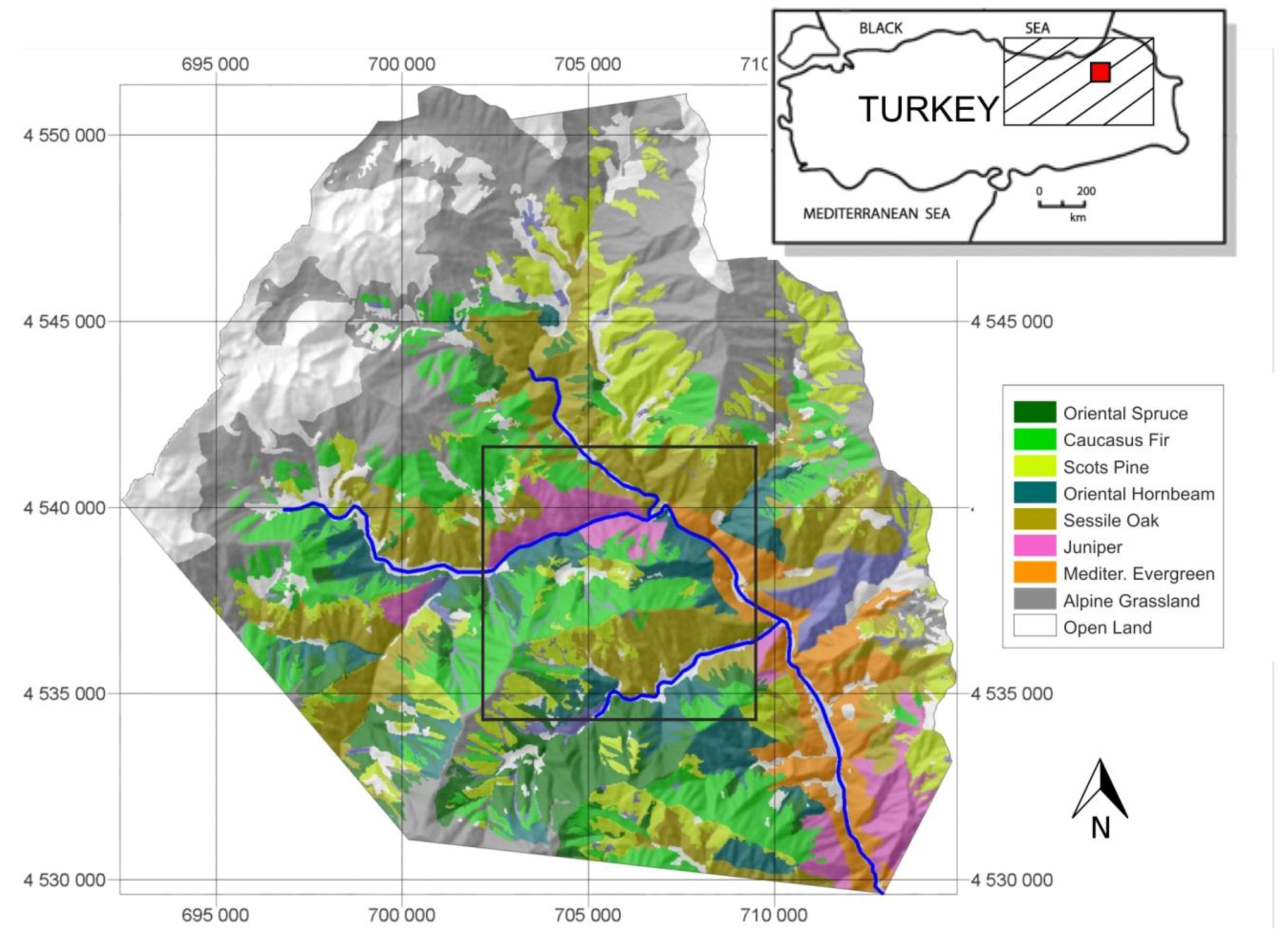
This study is conducted in the “Kaçkar Mountains Sustainable Forest Use and Biodiversity” Project Area [56] (Figure 1) which is remarkable with its natural old-growth forests, high plant diversity with many endemics and outstanding wildlife. The region is, however, subject to degradation and is currently facing threats that would cause irreversible changes to the forest ecosystem. These major threats are uncontrolled tourism, unlawful hunting, ineffective protection, illegal logging, and hydro electric station (HES) schemes.
3. Method
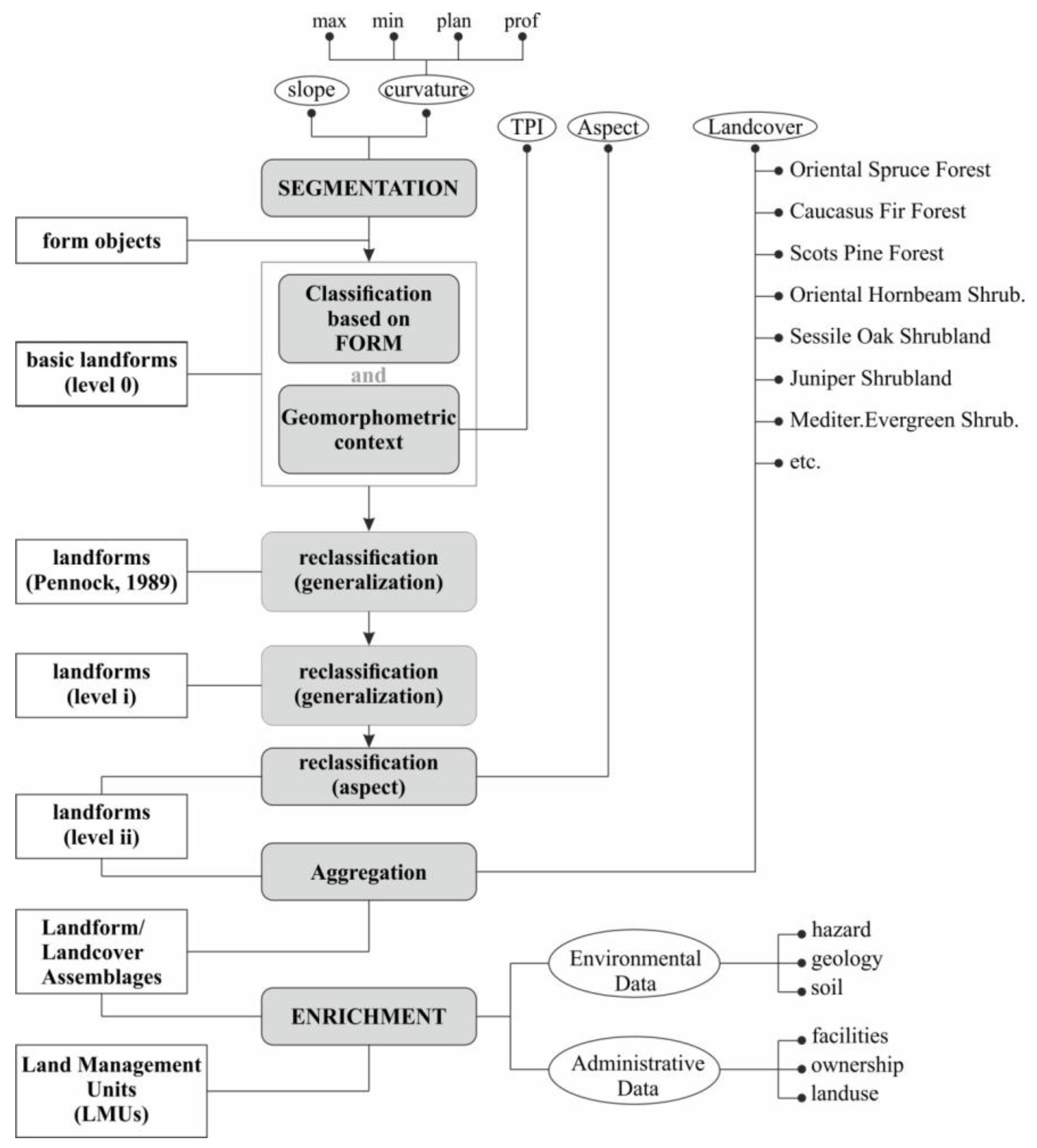
This study aims at delineating ecologically relevant LMUs with relational multi-level information that is suitable for land management, planning and conservation purposes. A strong relationship between landform and landcover is the rationale behind ecologically relevant Land Management Units (LMUs) [57]. Therefore, LMUs are based on landform/landcover assemblages, an aggregation of landforms and landcover information. The proposed method is applied to a site with rough topography and vegetation dominated by forests and shrublands that exhibits a wide range of possible combinations of landform, soil and vegetation types. The method adopts a stepwise approach to transition from simple form objects to enriched LMUs and can be divided broadly into three stages. A flowchart of the method can be seen in Figure 2.
The first stage is automated classification of the landscape into ecologically significant landforms. An object-based classification is performed through Geographic Object-Based Image Analysis (GEOBIA) using DTMs. Segmentation of DTMs including slope and curvature produces form objects that represent the geometric form of the landscape. Segmentation scale is essential for producing classes at a relevant scale which is designated as the landscape scale in the study. Sensitivity of landform classes to changes in the segmentation scale is tested by comparing a series of scales. Due to ambiguities in landforms both in attribute and geographical space, a fuzzy classification is employed to construct landform classes from initial form objects. Statistical significance of these classes was also tested. Landform classes based on geometric form were then reclassified to generate ecologically significant landform classes that utilize relative position and aspect of the terrain.
The second stage of the method involves aggregating landform classes with landcover information to constitute landform/landcover assemblages. Correlation and statistical relevance between landform types and the local vegetation types were reported with correlation measures and descriptive statistics. Relationship between landform and landcover in the study area rationalizes the idea of landform/landcover assemblages.
In the final and the third stage, other environmental, socio-economic and cultural data as input are transferred to enrich the assemblages, resulting in final LMUs that carry useful information for the conservation area at multiple levels to aid in decision making.
3.1. Data and Materials
3.1.1. Digital Terrain Models (DTMs)
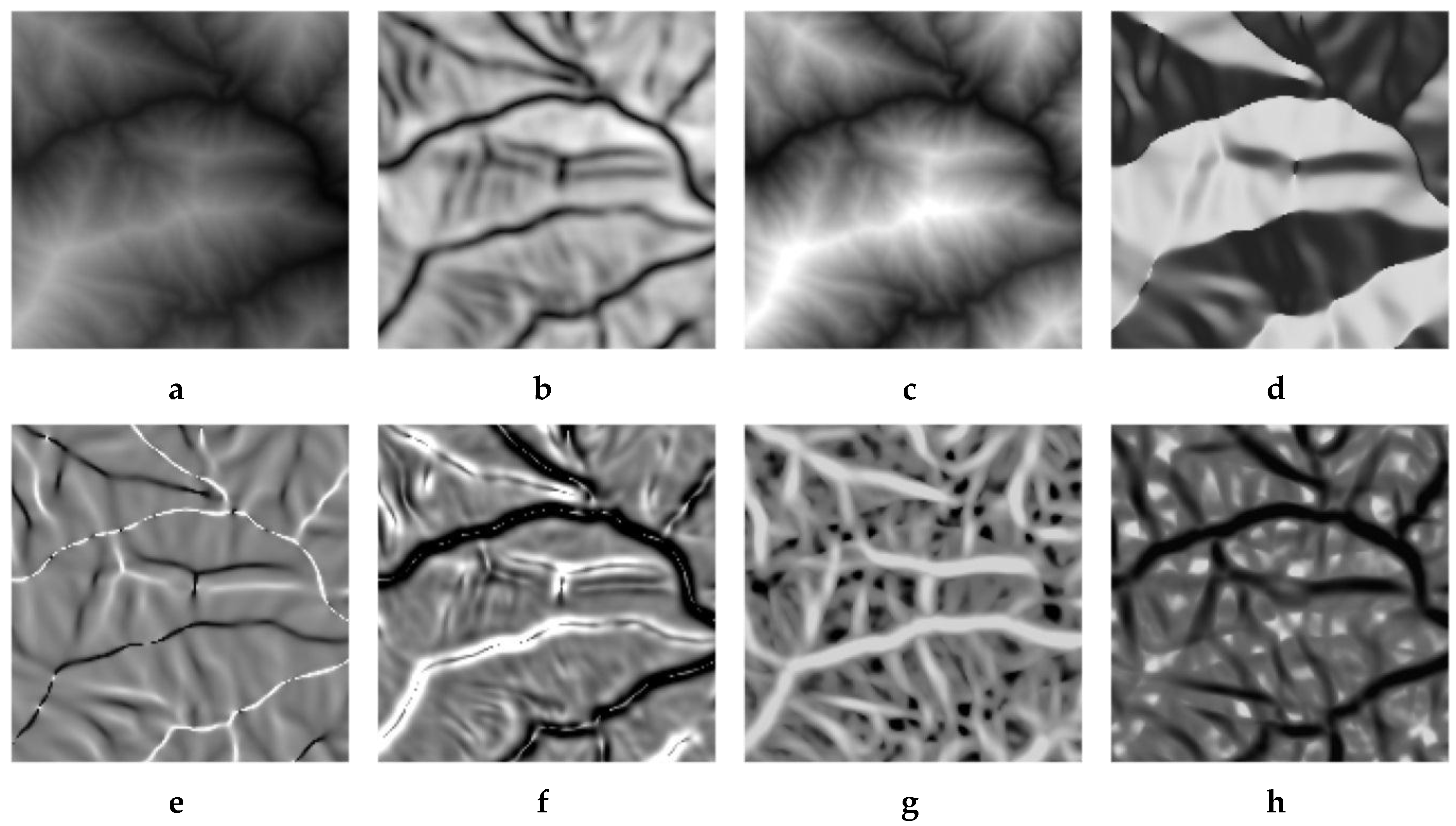
DTMs including slope, curvature, Topographic Position Index (TPI), and aspect are known to have strong control over environmental conditions through complex interactions. Fundamental DTMs used in the study are “slope”, “curvature” that represents geometric form and “TPI” that represents the relative position of terrain. Aspect is utilized to produce landform facets that govern major ecological functions. The Digital Elevation Model (DEM) at a resolution of 25 m generated out of 1/25,000 topographic contours with “topogrid” module of ArcGIS (an implementation of AnuDEM [58] constitutes the source of all of the Digital Terrain Models (DTMs) used in this study. DTMs are calculated at window size of 25 × 25 (225 × 225 m) so as to represent the surface at a landscape scale. Topographic contours (1/25,000 scale) with a 10-m vertical interval are quite appropriate to make a classification at Mesorelief A scale (described range covers topographic maps of 1/5000 to 1/50,000 [59] and pertain to a scale defined by ecologists where the majority of land surface processes that have significance in earth sciences takes place. Moreover, 1/25,000-scaled topographic maps are the standard maps that cover the whole country and they are widely available. Slope and four curvature DTMs that represent planar and vertical convexities of surfaces namely: maximum curvature, minimum curvature, plan curvature and profile curvature are produced in Landserf 2.3—a freeware by Wood [60] which enables use of user-defined window size for various derivative calculation at particular scales. Relative terrain position is calculated with Topographic Position Index (TPI) which is an ArcView extension developed by Jenness Enterprices [61]. Cosine of aspect was used instead of raw aspect values to represent slope azimuth as north facing or south facing. Original data values are [0, 34] for slope and [−10, +10] for four curvature types. Provided that data ranges of slope and curvature types are comparable, original data values were used for segmentation. However for classification, DTMs including slope, curvature types, TPI and aspect were normalized into [0, 1], or [−1, +1] (for curvature) ranges to ensure that the classification will work with the same thresholds at other case areas as well. The DEM of a selected region of the study area and DTMs which were utilized for the study are depicted in Figure 3. The selected region is a sample area for display purposes where analyses were conducted for whole study area (Figure 1).
3.1.2. Landcover
Landcover data for the study area were produced by the Nature Conservation Centre [62] for “Kackar Mountains Sustainable Forest Use and Biodiversity Project” based on Forest inventory maps at a 1/25,000 scale produced from aerial photos and CORINE 2006. CORINE landcover was utilized for general classes, while forest inventory maps were used to discriminate physiognomic classes. Results were updated for changes with satellite images (Landsat). Landcover with an associated legend of vegetation types of the study area can be seen in Figure 1. The CORINE accuracy requirement is set as 85% [63]. Although the accuracy of landcover for the study area is not systematically evaluated, it is anticipated that the accuracy is not lower than 85%, as CORINE was the basis of the landcover data.
The classification system is based on the physiognomy of the vegetation in the first level and floristic features according to dominant species and associated species in the second level [64]. The final map has a hierarchical structure that can be used in different scales and for forestry applications. It bears five different management purposes such as habitat suitability modelling, protected area zoning, physiognomic classes, twelve physiognomic subclasses, and 113 alliances. However, for this study, 113 alliance types were practically combined into 7 major landcover types as a high number of alliances may create noise in interpretation of the results. Major landcover types obtained through combination of alliances are as follows: Oriental Spruce (Picea orientalis L.) Forest, Caucasus Fir (Abies nordmanniana Mattf) Forest, Scots Pine (Pinus sylvestris L.) Forest, Oriental Hornbeam (Carpinus orientalis Mill.) Shrubland, Sessile Oak (Quercus petrea (Mattuschka) Lieb) Shrubland Juniper Shrubland (Juniperus sp.), Mediterranean evergreen shrubland and Alpine grassland.
3.2. Landform Objects (Segmentation)
Landform objects rather than individual pixels were utilized as a basis for classification in this study as they better conform to land features and have the ability to connect via a multi-level hierarchy [65]. Slope and four curvature types (maximum, minimum, plan, profile) that describe form [59] were used as input into the segmentation process. The “multiresolution segmentation” that adopts a region growing algorithm embedded in eCognition software was used in this study. Other segmentation algorithms, Chessboard and Quadtree-Based segmentation produce rectangular objects that have poor relevance to landform shapes. The spectral Difference Algorithm utilizes a threshold as a heterogeneity measure, a statistical class border that is hardly stable and extremely case-specific. Nevertheless, a prototype object definition that reflects the central tendency of features or properties of “real” entities [66] is more suitable for this study as will be mentioned in the Section 3.3 Landform Classification. Multiresolution segmentation is adopted among other segmentation algorithms for its flexibility in producing admired size and shape of segmentation, hierarchical levels in segmentation and transferring of fuzzy semantics for describing central tendencies to belonging to a class.
The segmentation algorithm merges individual pixels in a pairwise fashion into larger objects until a heterogeneity threshold defined by the user is reached. Given the slope and four curvature types that describe the geometric form of land surface, land is segmented into homogeneous “landform objects” with a multiresolution segmentation algorithm. All input layers (slope and four curvatures) were weighted the same. Heterogeneity criteria are controlled by a set of parameters: (i) scale parameter; (ii) weight of the spectral attribute versus shape; (iii) within shape criteria; weight of compactness versus smoothness [67]. The scale parameter determines the average size of the image objects. Segmentation accuracy and the overall effect of object-based classification are dependent on the segmentation scale [68]. Therefore, a series of scales (1 to 19) is explored to designate a medium segmentation level that does not over segment the land into very small objects or produce large objects that have high heterogeneity and exceed class sizes. Other parameters, i.e., the shape criterion, is set to 0.1, which automatically gives the weight of 0.9 to color/spectral values that are morphometric DTMs, and the compactness parameter was set to 0.5 that gives equal weight to compactness or smoothness.
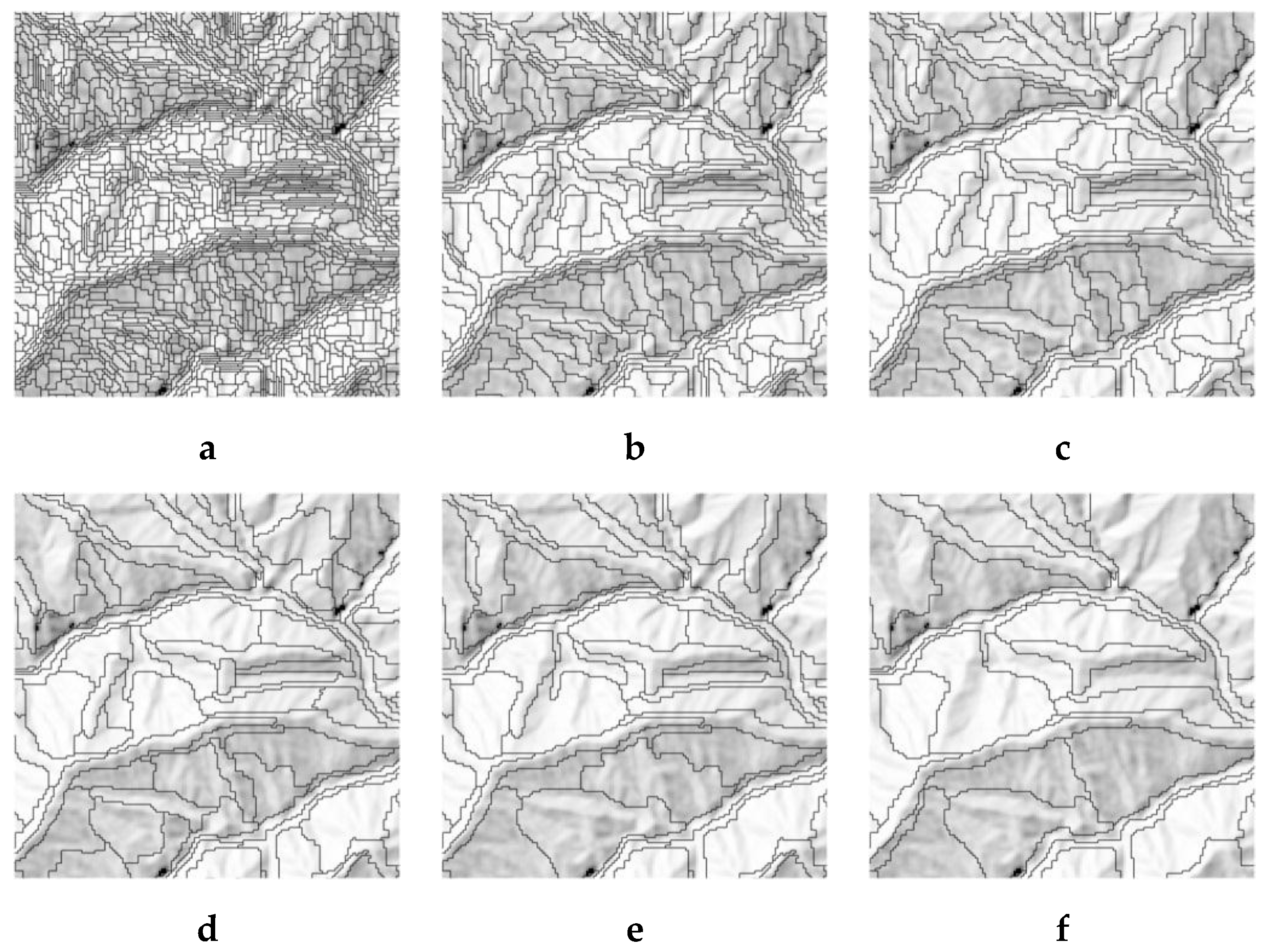
For segmentation, usually a series of trial and error procedures is suggested; however, there are tools to explore an optimal segmentation, i.e., “Estimation of Scale Parameter (ESP)” introduced by [69]. ESP that builds on the idea of “Local Variance” (LV) is employed for this study to obtain optimum scale out of a range of scales [1, 19]. The LV value is calculated as the average of all objects’ standard deviation. Accordingly, particular scale or scales where the rate of change of LV flattens out or drops indicates the optimum scale. Figure 4 illustrates the rate of change (ROC) of LV for successively increasing segmentation scales for the case. Unitless scale 8 portrays an initial drop and then flattening out and hence points out the proper scale that represents the characteristic size of the features in the dataset. Results of the segmentation at scales 2, 5, 8, 11, 14, and 17 for the sample area can be seen in Figure 5. According to the results segmentation, scale parameter 8 is visually more compatible to represent landform features at the landscape scale.
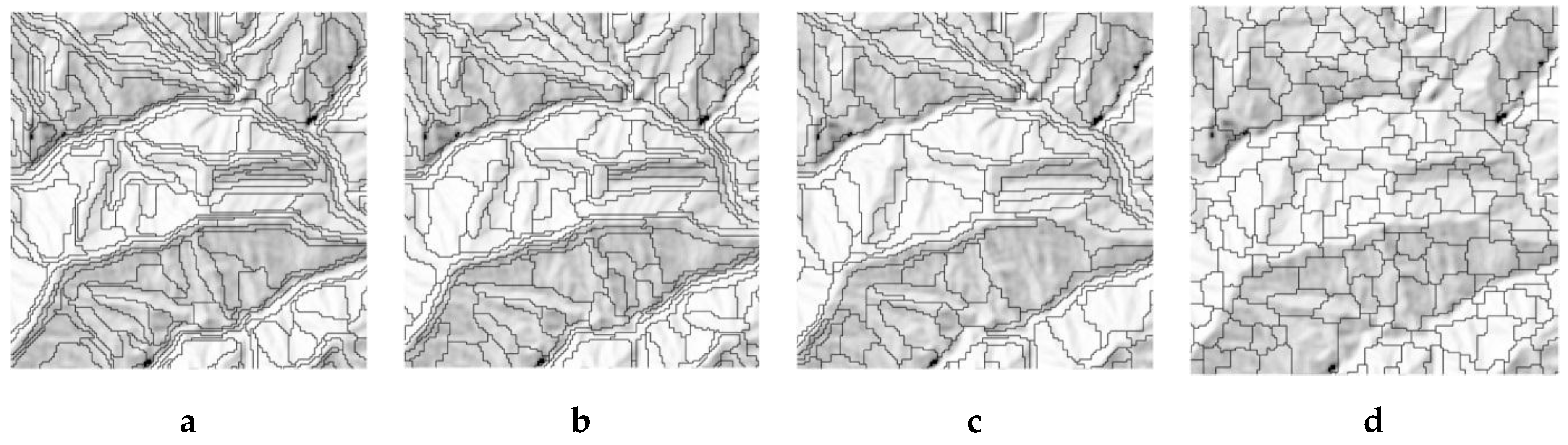
The segmentation parameters shape and compactness were also tested for the segmentation scale “8”. Changing the weight of compactness at the expense of smoothness did not significantly alter the results (Figure 6). However, an increased weight of shape is observed as posing misrepresentative objects of terrain features. This is attributed to the continuous nature of terrain which does not pose regular 2D shapes as could be observed in satellite imageries.
3.3. Landforms (Classification)
3.3.1. Basic Landforms (Level 0)
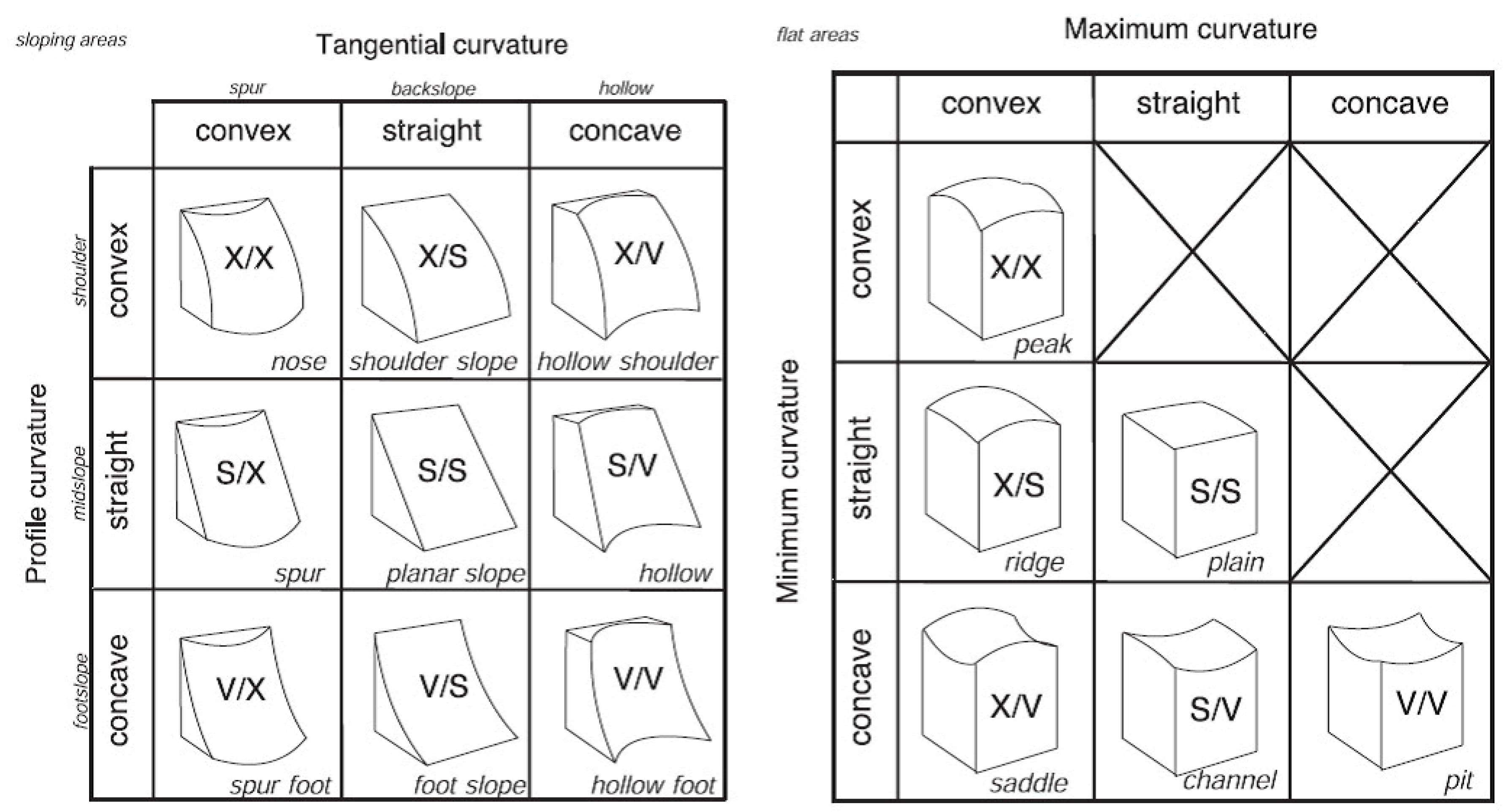
DTMs do not usually portray significant data clusters that correspond to particular landforms, as landforms ontologically are not “real” objects with crisp distinctions. Class definitions that describe central tendency to the prototypes for this study were built via Semantic Import (SI) which employs fuzziness to maintain indeterminate boundary conditions. Classification for the study comprises a series of classification and generalization procedures. Initially, objects gathered out of segmentation are classified based on local geometry to derive “15” basic form objects [59] (Figure 7). This scheme includes all possible combinations of form and is thus very appropriate for an exhaustive, general geomorphometric classification. These basic forms can also serve as basis for other classification schemes through generalization and reclassification.
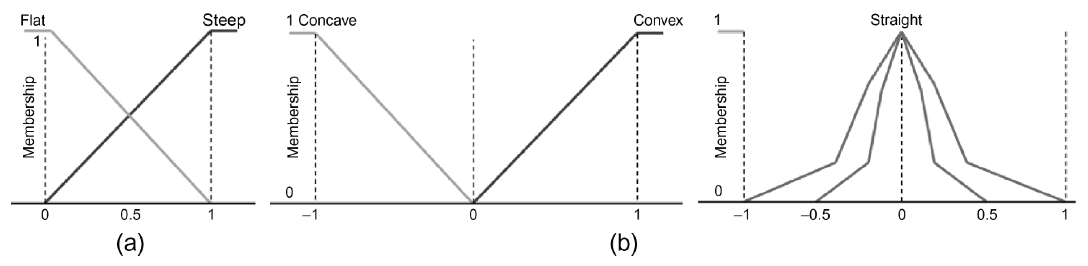
Surface parameters, slope and curvature, are descriptors of form. Slope quantifies whether topography is flat or sloping. Sloping areas are then assigned to nine classes according to plan and profile curvature, and flat areas are assigned to six classes according to minimum and maximum curvature (Figure 7). Morphometric DTMs with normalized values were used as input into fuzzy classification. Linear functions were used for importing semantics for flatness versus steepness in slope (Figure 8a). Curvedness for curvatures was also represented by a linear function. The frequency distribution of curvature parameters is bell-shaped with most of the values clustered around 0 and is therefore represented with a simple Gaussian curve. A narrow version is employed to describe straightness in planar forms: “plain” and “planar slope.” All of the 15 landforms are described with membership functions (Figure 8). Accordingly, form “peak” is defined as having membership of 1 for flatness of slope, and membership of 1 for convexness both in maximum and minimum curvature.
Classification based on local geometry produces classes that are “morphometric” rather than geomorphometric [60]. Landforms, however, have specific organization, where for instance, peaks and ridges are at the crests of hills and mountains; hence, they are positioned at the highest positions. Therefore, it is essential to make a reclassification to verify that the geometric classes are at their right position across the landscape. To implement this, the Topographic Position Index (TPI) is utilized. TPI determines relative position in downslope sequence, e.g., “shoulder” is a convex hillslope form located at relatively higher positions across the landscape characterized by high TPI values. This means if a geometric shoulder form is found in a region with low TPI values, it has to be reclassified to a proper footslope class according to geomorphometric context. Classification based on local geometry and geomorphometric context produces “basic landform classes” [43] depicted as “Level 0” in Figure 2 (Flowchart).
3.3.2. Ecologically Significant Landforms
Landforms
Seven landform classes of Pennock et al. [70] that depict ecologically critical landform classes were derived by reclassifying Basic Landforms (Level 0) to generalize them as shown in Table 1, 2nd column. The landform model of Pennock et al., which exhaustively covers the topography as landform classes that are significant for ecological processes, is adopted for this study. Pennock et al. [70] classified nine three-dimensional sloping classes by measures of slope, plan and profile curvature and two leveling classes, namely, crest and channel. Landforms are described by rate of change of slope in both vertical and horizontal planes. This scheme is also compatible with the scheme of Ruhe [27] and Dikau [59] which represents form only, and the scheme of Pennock et al., which represents terrain position information, making it suitable for use in ecological classification studies [10]. Pennock et al.’s landform classes are shown as “landforms (Pennock et.al., 1989)” [70] in Table 1.
Landforms (Level i)
Pennock et al.’s landform classes are further reorganized so as to represent more simplified landforms (level i, Table 1). Level i landforms simply differ from landforms of Pennock et al. in terms of generalized shoulder and footslope classes. Convexities and concavities in these classes are found to be less significant than in the backslope class, so they were grouped into single forms, “shoulder” or “footslope” ignoring their horizontal curvature. These landform classes are shown as “landforms (level i)” in Table 1.
Landforms (Level ii)
This classification is based on the form facet model [59]. Aspect information that is critical for energy, i.e., heat and light, is further integrated into the classification. The classification was implemented to produce landform facets or landform+aspect classes (level ii) as shown in the 4th column in Table 1. Sloping landforms, shoulders and backslopes were subdivided as north facing (e.g., Backslope North), south facing (e.g., backslaps South), or neither (e.g., Backslope). Footslopes are assumed to have low slopes with undefined aspect. These landform classes are shown as “landforms (level ii)” in Table 1.
Level ii landforms of the case area were assessed using evaluation reports from a group of earth scientists. Both the level i and level ii classes in Table 1 are tested for their relationship with landcover classes in this study. Outcomes of the two evaluations are presented in the Results section.
3.3.3. Landform/Landcover Assemblages (Aggregation)
Landcover for the study area is a polygon layer, and it is utilized in the aggregation process as a boundary condition. Therefore, initial landform objects besides having boundaries that determine homogeneous landform units, are merged with boundaries introduced by landcover types. This spatial information further provides easy transfer of landcover types into objects, as each object carries boundary conditions belonging to both landforms and landcover. If a vegetation type partially coincides with a landform object, only the major landcover type coinciding with the object is transferred to the specific polygon for practical reasons.
A subsequent procedure focuses on the aggregation of landform and landcover into meaningful assemblages. This higher level classification is aimed at deriving coarser units of landscape out of contiguous objects that are common in both landform and landcover. A substantial generalization after the merge operation was performed to remove sliver polygons, and polygons smaller than the mapping unit that is accepted as the smallest island polygon in the landcover data. A line simplification operation smooths the line for zig-zag pattern. Borders, if any, between the same landform/landcover class polygons were dissolved (Figure 9). As a consequence, the number of objects is reduced and objects become larger without any loss of information. Landform/landcover assemblages are possible combinations of landform and landcover, such as, ”Oriental Spruce Forest at Shoulder North” that represents north-facing shoulder slopes covered by Oriental Spruce forest.
3.3.4. Land Management Units (LMUs) (Enrichment)
The final step is the enrichment of landform/landcover assemblages with other available information. Soil, parent material, hazards, land use types, endangered species, ownership etc. are assigned to each object of common landform and landcover. Landform/landcover assemblages carry useful information on potentials of land and describe ecological conditions. Additional information brings a multilayered information content that can be efficiently utilized for management purposes. Each LMU, besides its own physical properties, becomes a carrier of other valuable thematic information. Landform/landcover assemblages in this study have been enriched using the available dataset of the study area.
4. Results
4.1. Basic Landforms’ Statistical Evaluation
Fuzzy morphometric classification can be evaluated for its stability and efficiency using some statistical techniques such as “classification stability”. “Classification stability” evaluates the differences in degrees of membership between the best classification result and the second best classification result for each object. A smaller value indicates more ambiguous classification. However, this technique is only applicable to fuzzy classes and therefore evaluation covers “basic landforms” only. Accordingly, the first five classes for stability are planar slope, foot slope, channel, “ridge”, and “shoulder”. These classes are separable from other classes given their statistical nature and class definitions. The last five classes beginning from the least stable are spur foot, hollow foot, hollow shoulder, nose, and saddle. These classes pose unsatisfactory classification statistics which can be reconsidered for improved consistency or they can be embedded into a larger class, for example, class “hollow foot” and “hollow shoulder” can be combined into a single hollow class. Most of these poorly classified classes were reclassified into a relevant general class (i.e., landforms of Pennock et al. [69] (level i) or landforms (level i) for stability reasons and general purpose of the study.
4.2. Landform Classes External Evaluation
An evaluation of landform classification results is implemented with volunteering geoscientists including two geologists, two geophysicists, and one geodesist experienced in morphometry. Stratified random points are generated given the class boundaries, so that each class can be represented with enough points—at least three for the smallest class. A total of 40 points for the case area is produced. Results show that the highest rate of consistency between the proposed landform classification (level ii) and the evaluators’ choice is for “Crest” and the lowest is for “Shoulder”. The following are the landforms sorted from highest to lowest for their rate of consistency according to the evaluators’ reports: Crest (80%), Shoulder_N (53.3%), Channel (46.7%), Footslope (37.5%), Backslope_N (35%), Backslope_S (32%), Shoulder_S (26.7%), Backslope (13.3%), Shoulder (0%).
Most of the inconsistency between the outcomes and the evaluators’ choices is noticed between the specific classes. Below is the pair of classes most mismatched and the number of mismatches between the two classes
Backslope North and Shoulder North, 9 mismatches
Backslope South and Footslope, 7 mismatches
Backslope North–Footslope, 6 mismatches
Footslope–Channel, 6 mismatches
Backslope–Backslope South, 5 mismatches
It can be understood from the geomorphometric context that four of the highest mismatches are between the classes neighboring in the vertical space. These are also a few mismatches between classes neighboring in the horizontal space, i.e., Backslope and Backslope South. This is to an extent tolerable as evaluators may not decide between the two classes because of the continuous transition between them.
4.3. Relevance of Landform/Landcover Assemblages
In order to assess the relationship between landform classes and the landcover classes in the study area, a statistical independence analysis was performed. The chi-square (χ2) test of independence is used to test for a statistically significant relationship between two categorical variables. Major landcover types and their relation to landforms, level i and level ii, are examined through the chi-squared test and to portray correlation, if any. Evaluations of the relationship between landcover and corresponding landform types show a significant relationship.
Eight landforms when combined with eight landcover types produce 64 possible combinations of landform and landcover classes. However, 58 actual combinations observed in the study area. About one third of them very small in size are ignored regarding a smallest mapping unit measure as a scale indicator, and 35 observed combinations of landform land cover remained. Landforms and landcover types in the area show significant correlation. Null hypothesis that ”the two categorical variable sets, landforms and landcover types are not related” is rejected at p = 0.001 at relevant degrees of freedom (Table 2). Chi-square values for landforms with aspect (level ii) yield higher values compared to landforms (level i). The relationship between landcover is far more than random for these landforms; therefore, they are used for coupling landcover types to produce landform/landcover assemblages. Chi-square is calculated for each landcover type (Table 2). Accordingly, Caucasian Fir, Oriental Spruce, Alpine grassland, Mediterranean shrubland and Scots Pine distribution is strongly correlated with the landform types. As Oriental Hornbeam and Juniper shrublands have wider ecological tolerance, they do not show strong correlation with specific landforms. Juniper shrublands are even uncorrelated with test statistics lower than the critical value. Inclusion of aspect information into landform classification influences the significance levels of relationships. Accordingly, Alpine grasslands, Mediterranean Shrubland, Oriental Hornbeam Shrubland do not vary with aspect whereas Oriental Spruce, Caucasian Fir, Scots Pine and Sessile Oak do.
Moreover, distribution of landforms for each landcover type has been examined and compared to the general distribution of the landforms (Level ii) for the whole study area (Table 3). Percentage ratios show that some of the landcover types have particular preferences of landforms. Oriental Spruce, Caucasian Fir and Oriental Hornbeam Shrublands mostly prefer north-facing slopes, whereas Sessile Oak Shrub and Juniper Shrub grow mainly on the south-facing slopes. Mediterranean shrub is settled on the footslopes as this species prefers warmer climatic conditions.
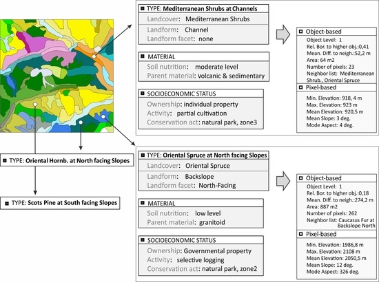
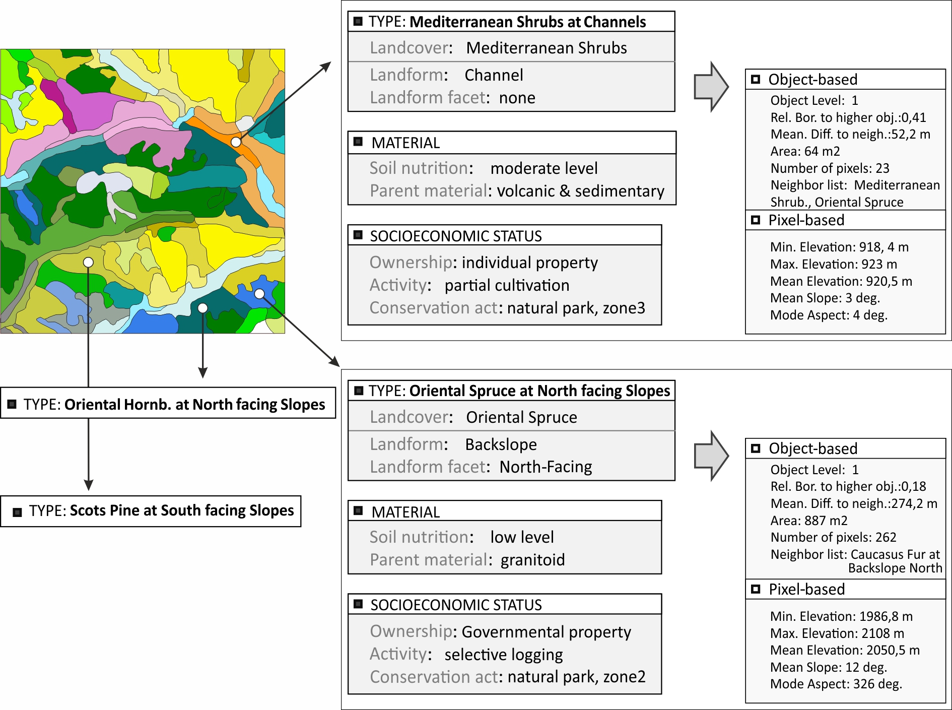
4.4. Structure of Geographic Database and LMUs
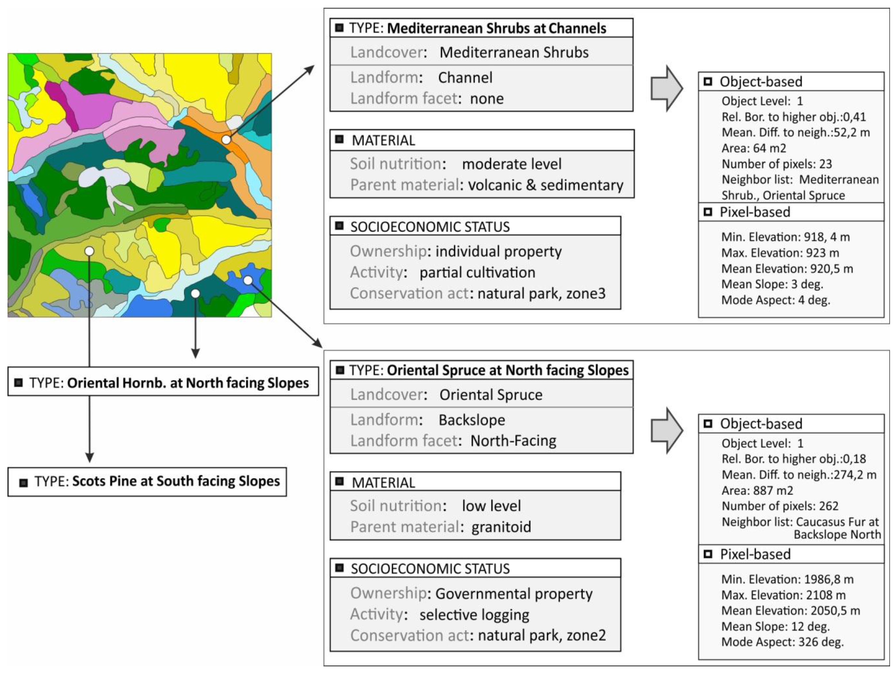
The method adopts a stepwise approach to transform simple form objects into data-rich LMUs. Selecting a LMU object in the final product, one can obtain from the relational database table its land use, landcover type, ownership, etc. (Figure 10). At the lower hierarchical levels, landform in either microform or form facet level can be reached. The lowest level information such as the mean slope and mean altitude of the individual objects can also be reached through a flexible environment of multi-resolution segmentation.
5. Conclusions
Many environmental factors influence the nature and management of ecosystems; however, topography synthesizes many of the other factors. Landforms influence and show covariance with a variety of site factors including micro-climate, soil thickness, nutrient regime, and vegetation composition. Hence, understanding landforms and geomorphological processes is essential to understanding the potentials of landscapes. Moreover, landforms are the most permanent and stable feature of the ecosystem and are relatively easy to identify in the field. Landforms in this study were produced through a series of classifications to produce ecologically significant landform types. The landforms proved statistical significance and they portray adequate consistencies with external evaluations made by earth scientists.
Landform and landcover are strongly related through complex interactions. This relationship quantified through statistical analysis for the study area supports and rationalizes the idea behind landform/ landcover assemblages as the basis for ecologically relevant Land Management Units (LMUs).
Landforms together with landcover in this study produce representative units for ecological conditions. These units may be the key for assessing habitat distribution, landscape composition or land use changes. Enrichment of those units into LMUs provides a formal background for further planning and management purposes in a multi-level hierarchy.
Ecologically sound LMUs are also necessary for effective communication and easy exchange of information between decision makers and land resources managers. LMUs reflect potential and actual condition of the pieces of land. The same classes of LMUs reflect similar land potentials and are expected to respond to particular decisions in a similar fashion. LMUs are foreseen as useful management units for the decision-making process, especially for the conservation of the study area. The method is not only limited to management of forest ecosystems and conservation but is also suitable for broader land planning, agriculture, and management actions. It is also possible to generate a higher level information product with additional data, in cases where available.
Acknowledgments
Landcover data used for in this paper were produced as part of the “Kaçkar Mountains Sustainable Forest Use and Biodiversity Project” supported by the EU and carried out by TEMA, DKM, METU, AKDD, OGM, DKMP. Uğur Zeydanlı as founder of DKM is acknowledged for providing land cover data and his support in interpreting the biological nomenclature in this study. Volunteering earth scientists İ. Talih Güven, Ercan Sangu, Ozan Arslan, Aziz Özyavaş, and Deniz Çakı are gratefully thanked for their evaluations of the landform classification results.
Conflicts of Interest
The author declares no conflict of interest.
References
- Zonneveld, I.S. Land Ecology; SPB Academic Publishing: Amsterdam, The Netherlands, 1995. [Google Scholar]
- Christian, C.S. The concept of land units and land systems. In Proceedings of the Ninth Pacific Congress, Bangkok, Thailand, 18 November–9 December 1957; Volume 20, pp. 74–81. [Google Scholar]
- Forman, R.T.T. Land Mosaics: The Ecology of Landscapes and Regions; Cambridge University Press: Cambridge, UK, 1995. [Google Scholar]
- McMahon, G.; Wiken, E.B.; Gauthier, D.A. Toward a Scientifically Rigorous Basis for Developing Mapped Ecological Regions. Environ. Manag. 2004, 34, S111–S124. [Google Scholar] [CrossRef]
- Eswaran, H.; Beinroth, F.H.; Virmani, S.M. Resource management domains: A biophysical unit for assessing and monitoring land quality. Agric. Ecosyst. Environ. 2000, 81, 155–162. [Google Scholar] [CrossRef]
- Baja, S.; Chapman, D.M.; Dragovich, D. A Conceptual Model for Defining and Assessing Land Management Units Using a Fuzzy Modeling Approach in GIS Environment. Environ. Manag. 2002, 29, 647–661. [Google Scholar] [CrossRef]
- Brown, G.; Raymond, C. The relationship between place attachment and landscape values: Toward mapping place attachment. Appl. Geogr. 2007, 27, 89–111. [Google Scholar] [CrossRef]
- The Natural Choice: Securing the Value of Nature, Department for Environment, Food & Rural Affairs (DEFR): 2011. Available online: https://www.gov.uk/government/uploads/system/uploads/attachment_data/file/228842/8082.pdf (accessed on 8 June 2017).
- Omernik, J.M. Ecoregions of the conterminous U.S. Ann. Assoc. Am. Geogr. 1987, 77, 118–125. [Google Scholar] [CrossRef]
- MacMillan, R.A.; Torregrosa, A.; Moon, D.; Coupé, R.; Philips, N. Automated predictive mapping of ecological entities. In Geomorphometry—Concepts, Software, Applications; Hengl, T., Reuter, H.I., Eds.; Elsevier: Amsterdam, The Netherlands, 2009; Chapter 24; pp. 551–578. [Google Scholar]
- Diaz-Balteiro, L.; Romero, C. Making forestry decisions with multiple criteria: A review and an assessment. For. Ecol. Manag. 2008, 255, 3222–3241. [Google Scholar] [CrossRef]
- MacMillan, R.A.; Moon, D.E.; Coupé, R.A. Automated predictive ecological mapping in a Forest Region of B.C., Canada, 2001–2005. Geoderma 2007, 140, 353–373. [Google Scholar] [CrossRef]
- Castillo-Rodriguez, M.; Lopez-Blanco, J.; Munoz-Salinas, E. A geomorphologic GIS-multivariate analysis approach to delineate environmental units, a case study of La Malinche volcano (central Mexico). Appl. Geogr. 2010, 30, 629–638. [Google Scholar] [CrossRef]
- Leibovici, D.G.; Jackson, M. Multi-scale integration for spatio-temporal ecoregioning delineation. Int. J. Image Data Fusion 2011, 2, 105–119. [Google Scholar] [CrossRef]
- Klingseisen, B.; Metternicht, G.; Paulus, G.; Wilson, D. Geomorphometric Landscape Analysis of Agricultural Areas and Rangelands of Western Australia. In Geopedology; Zinck, J.A., Metternicht, G., Bocco, G., Del Valle, H.F., Eds.; Springer: Berlin, Germany, 2016; pp. 361–376. [Google Scholar]
- Cooke, R.U.; Doornkamp, J.C. Geomorphology in Environmental Management: An Introduction; Clarendon Press: Oxford, UK, 1974. [Google Scholar]
- Verstappen, H.T.; van Zuidam, R. The ITC System of Geomorphologic Survey: A Basis for the Evaluation of Natural Resources and Hazards; ITC Publ. N. 10; ITC (International Institute for Geo-Information Science and Earth Observation): Enschede, The Netherlands, 1991; p. 89. [Google Scholar]
- López-Blanco, J.; Villers-Ruiz, L. Delineating boundaries of environmental units for land management using a geomorphological approach and GIS-a study in Baja California, Mexico. Remote Sens. Environ. 1995, 53, 109–117. [Google Scholar] [CrossRef]
- Butler, D. Geomorphic process-disturbance corridors: A variation on a principle of landscape ecology. Prog. Phys. Geogr. 2001, 2, 237–248. [Google Scholar]
- Gessler, P.E.; Moore, I.D.; McKenzie, N.J.; Ryan, P.J. Soil-landscape modelling and spatial prediction of soil attributes. Int. J. Geogr. Inf. Sci. 1995, 9, 421–432. [Google Scholar] [CrossRef]
- McKenzie, N.J.; Ryan, P.J. Spatial prediction of soil properties using environmental correlation. Geoderma 1999, 89, 67–94. [Google Scholar] [CrossRef]
- Wilson, J.P.; Gallant, J.C. Digital Terrain Analysis. In Terrain Analysis: Principles and Applications; Wilson, J.P., Gallant, J.C., Eds.; Wiley: New York, NY, USA, 2000; pp. 1–29. [Google Scholar]
- Moore, I.D.; Gessler, P.E.; Nielsen, G.A.; Peterson, G.A. Soil attribute prediction using terrain analysis. Soil Sci. Soc. Am. J. 1993, 57, 443–452. [Google Scholar] [CrossRef]
- Austin, M.P.; Smith, T.M. A new model for the continuum concept. Vegetatio 1989, 83, 35–47. [Google Scholar] [CrossRef]
- Theobald, D.M.; Harrison-Atlas, D.; Monahan, W.B.; Albano, C.M. Ecologically-relevant maps of landforms and physiographic diversity for climate adaptation planning. PLoS ONE 2015, 10, 1–17. [Google Scholar] [CrossRef] [PubMed]
- Reuter, H.I.; Wendroth, O.; Kersebaum, K.C. Optimisation of relief classification for different levels of generalisation. Geomorphology 2006, 77, 79–89. [Google Scholar] [CrossRef]
- Ruhe, R.V. Geomorphology, Geomorphologic Processes and Surficial Geology; Houghton Mifflin: Boston, MA, USA, 1975. [Google Scholar]
- Ventura, S.J.; Irvin, B.J. Automated Landform Classification Methods for Soil-Landscape Studies. In Terrain Analysis Principals and Applications; Wilson, J.P., Gallant, J.C., Eds.; John Wiley & Sons: New York, NY, USA, 2000; pp. 245–294. [Google Scholar]
- Asselen, S.; Verburg, P. A Land System representation for global assessments and land-use modeling. Glob. Chang. Biol. 2012, 18, 3125–3148. [Google Scholar] [CrossRef]
- Tagil, S.; Jenness, J. GIS-Based Automated Landform Classification and Topographic, Landcover and Geologic Attributes of Landforms around the Yazoren Polje, Turkey. J. Appl. Sci. 2008, 8, 910–921. [Google Scholar] [CrossRef]
- Temimi, M.; Leconte, R.; Chaouch, N.; Sukumal, P.; Khanbilvardi, R.; Brissette, F. A combination of remote sensing data and topographic attributes for the spatial and temporal monitoring of soil wetness. J. Hydrol. 2010, 388, 28–40. [Google Scholar] [CrossRef]
- Greve, M.H.; Kheira, R.B.; Greve, M.B.; Bocher, P.K. Quantifying the ability of environmental parameters to predict soil texture fractions using regression-tree model with GIS and LIDAR data: The case study of Denmark. Ecol. Indic. 2012, 18, 1–10. [Google Scholar] [CrossRef]
- Tabik, S.; Villegas, A.; Zapata, E.L.; Romero, L.F. A Fast GIS-tool to Compute the Maximum Solar Energy on Very Large Terrains. Procedia Comput. Sci. 2012, 9, 364–372. [Google Scholar] [CrossRef]
- Simbahan, G.C.; Dobermann, A. An algorithm for spatially constrained classification of categorical and continuous soil properties. Geoderma 2006, 136, 504–523. [Google Scholar] [CrossRef]
- Beier, P.; Brost, B. Use of Land Facets to Plan for Climate Change: Conserving the Arenas, Not the Actors. Conserv. Biol. 2010, 24, 701–710. [Google Scholar] [CrossRef] [PubMed]
- Niesterowicz, J.; Stepinski, T.F. Regionalization of multi-categorical landscapes using machine vision methods. Appl. Geogr. 2013, 45, 250–258. [Google Scholar] [CrossRef]
- Hay, G.J.; Castilla, G. Object-based Image Analysis (OBIA), Strengths, Weakness, Opportunities, and Threats (SWOT). In Proceedings of the 1st International Conference on Object-based Image Analysis (OBIA2006), Salzburg University, Salzburg, Austria, 4–5 July 2006. [Google Scholar]
- Blaschke, T. Object based image analysis for remote sensing. ISPRS J. Photogramm. Remote Sens. 2010, 65, 2–16. [Google Scholar] [CrossRef]
- Fisher, P.; Wood, J.; Cheng, T. Where is Helvellyn? Fuzziness of multi-scale landscape morphometry. Trans. Inst. Br. Geogr. 2004, 29, 106–128. [Google Scholar] [CrossRef]
- Myint, S.W.; Gober, P.; Brazel, A.; Grossman-Clarke, S.; Weng, Q. Per-pixel vs. object-based classification of urban land cover extraction using high spatial resolution imagery. Remote Sens. Environ. 2011, 115, 1145–1161. [Google Scholar] [CrossRef]
- Blaschke, T.; Hay, G.J.; Kelly, M.; Lang, S.; Hofmann, P.; Addink, E.; Feitosa, R.Q.; van der Meer, F.; van der Werff, H.; van Coillie, F.; et al. Geographic Object-Based Image Analysis—Towards a new paradigm. ISPRS J. Photogramm. Remote Sens. 2014, 87, 180–191. [Google Scholar] [CrossRef] [PubMed]
- Cheng, G.; Han, J. A survey on object detection in optical remote sensing images. ISPRS J. Photogramm. Remote Sens. 2016, 117, 11–28. [Google Scholar] [CrossRef]
- Gerçek, D.; Toprak, V.; Strobl, J. Object-Based classification of Landforms based on their Local Geometry and Geomorphometric Context. Int. J. Geogr. Inf. Sci. 2011, 25, 1011–1023. [Google Scholar] [CrossRef]
- Drăguţ, L.; Eisank, C. Automated object-based classification of topography from SRTM data. Geomorphology 2012, 141–412, 21–33. [Google Scholar] [CrossRef] [PubMed]
- Drăguţ, L.; Csilik, O.; Minár, J.; Evans, I.S. Land-surface segmentation to delineate elementary forms from Digital Elevation Models. In Proceedings of the Geomorphometry 2013, Nanjing, China, 16–20 October 2013. [Google Scholar]
- Guibert, E.; Moulin, B. Towards a Common Framework for the Identification of Landforms on Terrain Models. Int. J. Geo-Inf. 2017, 6, 1–21. [Google Scholar]
- Smith, B.; Mark, D.M. Do mountains exist? Towards an ontology of landforms. Environ. Plan. B Plan. Des. 2003, 30, 411–427. [Google Scholar] [CrossRef]
- Williamson, T. Vagueness; Routledge: New York, NY, USA, 1994; p. 306. [Google Scholar]
- Schmidt, J.; Hewitt, A. Fuzzy land element classification from DTMs based on geometry and terrain position. Geoderma 2004, 121, 243–256. [Google Scholar] [CrossRef]
- Gorini, M.A.V.; Mota, G.L.A. Dealing with double vagueness in DEM morphometric analysis. Int. J. Geogr. Inf. Sci. 2016, 30, 1644–1666. [Google Scholar] [CrossRef]
- Pfeffer, K.; Pebesma, E.J.; Burrough, P.A. Mapping alpine vegetation using vegetation observations and topographic attributes. Landsc. Ecol. 2003, 18, 759–776. [Google Scholar] [CrossRef]
- Bailey, R.G. Ecosystem Geography; Springer: New York, NY, USA, 1996. [Google Scholar]
- Bayrakdar, C.; Özdemir, H. Kaçkar Dağı’nda Bakı Faktörünün Glasiyal ve Periglasiyal Topografya Gelişimi Üzerindeki Etkisi. Türk Corafya Dergisi 2010, 54, 1–13. [Google Scholar]
- İklim: Yusufeli–İklim Grafiği, Sıcaklık Grafiği, İklim Tablosu - Climate-Data.org. Available online: https://tr.climate-data.org/location/665980/ (accessed on 7 March 2017).
- YayinDosya_L2OSaIgK.pdf. Available online: http://www.dkm.org.tr/Dosyalar/YayinDosya_L2OSaIgK.pdf (accessed on 7 March 2017).
- Doğa Koruma Merkezi–Kaçkar Ormanları. Available online: http://dkm.org.tr/Projeler/68/kackar-ormanlari (accessed on 7 March 2017).
- Gerçek, D.; Zeydanlı, U. Object-based classification of Landscape into Land management Units (LMUs), Geographic Object based Image Analysis. In Proceedings of the Third International Conference on All Aspects of Geographic Object-Based Image Analysis, Gent, Belgium, 29 June–2 July 2010. [Google Scholar]
- Hutchinson, M.F. A new procedure for gridding elevation and stream line data with automatic removal of spurious pits. J. Hydrol. 1989, 106, 211–232. [Google Scholar] [CrossRef]
- Dikau, R. The application of a digital relief model to landform analysis. In 3D Applications in Geographic Information Sytems; Raper, J.F., Ed.; Taylor&Francis: Abingdon, UK, 1989; pp. 51–77. [Google Scholar]
- Wood, J.D. The Geomorphological Characterization of Digital Elevation Models. Ph.D. Thesis, University of Leicester, Leicester, UK, 1996. [Google Scholar]
- Jenness, J. Topographic Position Index (tpi_jen.avx) Extension for ArcView 3.x, v. 1.3a; Jenness Enterprises: Flagstaff, AZ, USA, 2006. [Google Scholar]
- Doğa Koruma Merkezi. Available online: http://www.dkm.org.tr/ (accessed on 8 June 2017).
- CORINE Land Cover. Available online: http://land.copernicus.eu/pan-european/corine-land-cover (accessed on 8 June 2017).
- Jennings, M.D. Modified UNESCO Natural Terrestrial Cover Classification. National Biological Survey; Idaho Cooperative Fish and Wildlife Research Unit: Moscow, ID, USA, 1999. [Google Scholar]
- Baatz, M.; Schäpe, A. Multiresolution Segmentation—An optimization approach for high quality multiscale image segmentation. In Angewandte Geographische Informationsverarbeitung XII; Strobl, J., Ed.; Wichmann: Heidelberg, Germany, 2000; pp. 12–23. [Google Scholar]
- Rosch, E.H. Natural categories. Cogn. Psychol. 1973, 4, 328–350. [Google Scholar] [CrossRef]
- Benz, U.C.; Hofmann, P.; Willhauck, G.; Lingenfelder, I.; Heyen, M. Multi-resolution, object-oriented fuzzy analysis of remote sensing data for GIS-ready information. ISPRS J. Photogramm. Remote Sens. 2004, 58, 239–258. [Google Scholar] [CrossRef]
- Addink, E.A.; de Jong, S.M.; Pebesma, E.J. The importance of scale in object based mapping of vegetation parameters with hyperspectral imagery. Photogramm. Eng. Remote Sens. 2007, 73, 905–912. [Google Scholar] [CrossRef]
- Drăguţ, L.; Tiede, D.; Levick, S.L. ESP: A tool for estimating the scale parameter for multiresolution image segmentation of remotely sensed data. Int. J. Geogr. Inf. Sci. 2010, 24, 859–871. [Google Scholar]
- Pennock, D.J.; Zebarth, B.J.; De Jong, E. Landform classification and soil distribution in Hummocky terrain, Saskatchewan, Canada. Geoderma 1987, 40, 297–315. [Google Scholar] [CrossRef]
Figure 1.
Study area and location. Rectangle represents the sample area for display purposes for the following figures.
Figure 1.
Study area and location. Rectangle represents the sample area for display purposes for the following figures.

Figure 2.
Flowchart of the method.

Figure 3.
DTMs of a sample area (a) DEM; (b) Slope; (c) Topographic Position Index (TPI); (d) Aspect; (e) Plan curvature; (f) Profile curvature; (g) Maximum curvature; (h) Minimum curvature.
Figure 3.
DTMs of a sample area (a) DEM; (b) Slope; (c) Topographic Position Index (TPI); (d) Aspect; (e) Plan curvature; (f) Profile curvature; (g) Maximum curvature; (h) Minimum curvature.

Figure 4.
Estimation of Scale Parameter (ESP) results for a range of scales (1–20) for the study area.
Figure 4.
Estimation of Scale Parameter (ESP) results for a range of scales (1–20) for the study area.

Figure 5.
Segmentation at scales: (a) 2; (b) 5; (c) 8; (d) 11; (e) 14; (f) 17.

Figure 6.
Segmentation at scale 8 with changes in shape and compactness parameters (a) shape: 0.1; compactness: 0.1; (b) shape 0.1, compactness: 0.5; (c) shape: 0.5, compactness: 0.1; (d) shape 0.5, compactness: 0.5.
Figure 6.
Segmentation at scale 8 with changes in shape and compactness parameters (a) shape: 0.1; compactness: 0.1; (b) shape 0.1, compactness: 0.5; (c) shape: 0.5, compactness: 0.1; (d) shape 0.5, compactness: 0.5.

Figure 7.
Fifteen “form elements” offered by [59] based on local geometry. (X = convex, V = concave, S = straight).
Figure 7.
Fifteen “form elements” offered by [59] based on local geometry. (X = convex, V = concave, S = straight).

Figure 8.
Membership functions used for fuzzy classification of basic landform classes. Membership function for (a) steepness or flatness and (b) curvedness or straightness.
Figure 8.
Membership functions used for fuzzy classification of basic landform classes. Membership function for (a) steepness or flatness and (b) curvedness or straightness.

Figure 9.
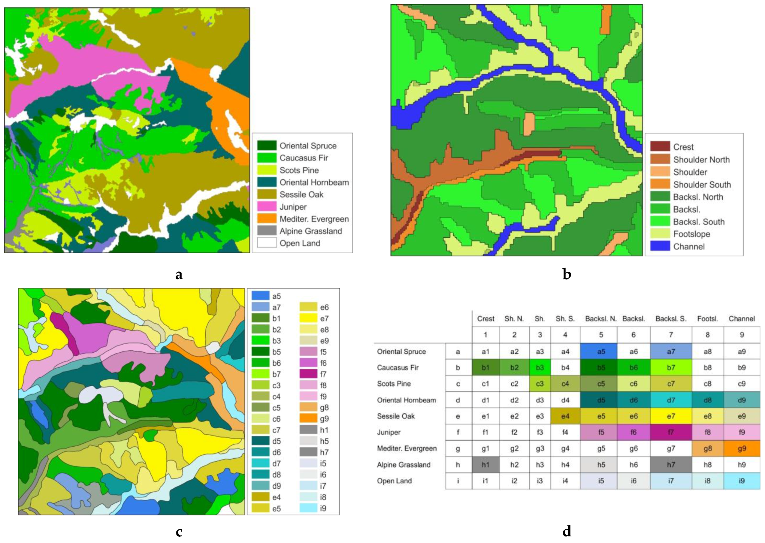
(a) Landcover classes; (b) Landform classes (level ii); (c) Landform/Landcover assemblages; (d) look-up table with colors for the Landform/Landcover assemblages.
Figure 9.
(a) Landcover classes; (b) Landform classes (level ii); (c) Landform/Landcover assemblages; (d) look-up table with colors for the Landform/Landcover assemblages.

Figure 10.
Four LMU records, two of which are appended for their attributes at class, object and pixel levels from the geodatabase of LMUs.
Figure 10.
Four LMU records, two of which are appended for their attributes at class, object and pixel levels from the geodatabase of LMUs.


Table 1.
Landform classes.
| Basic Landforms (Level 0) | Landforms Pennock (1987) | Landforms (Level i) | Landforms (Level ii) |
|---|---|---|---|
| Peak | Crest | Crest | Crest |
| Ridge | |||
| Saddle | |||
| Plain * | |||
| Nose | Divergent Shoul. | Shoulder | Shoulder North |
| Shoulder slope | Planar Shoul. | Shoulder | |
| Hollow shoulder | Convergent Shoul. | Shoulder South | |
| Spur | Divergent Backsl. | Divergent Backsl. | Backsl. North |
| Planar slope | Planar Backsl. | Planar Backsl. | Backsl. |
| Hollow | Convergent Backsl. | Convergent Backsl. | Backsl. South |
| Spur foot | Divergent Footslope | Footslope | Footslope |
| Foot slope | Planar Footslope | ||
| Hollow foot | Convergent Footsl. | ||
| Pit | Channel | Channel | Channel |
| Channel | |||
| Plain * | |||
| 15 classes | 11 classes | 7 classes | 9 classes |
* class “plain” exists both in upper and lower features.
Table 2.
Chi-square test for Landforms vs. landcover.
| Landcover Type | Chi-Square for Landforms (Level i) | Chi-Square for Landforms (Level ii) |
|---|---|---|
| Oriental Spruce Forest | 28.34921 | 140.2911 |
| Caucasus Fir Forest | 114.6288 | 273.9556 |
| Scots Pine Forest | 74.74214 | 195.352 |
| Oriental Hornbeam Shrubland | 31.48607 | 37.0501 |
| Sessile Oak Shrubland | 174.9733 | 260.0567 |
| Juniper Shrubland | 22.43 | 25.52 |
| Mediterranean Evergreen Shrubland | 302.7082 | 306.8828 |
| Test statistic | critical value for p = 0.001 at d.f. = 6 is 22.46 | critical value for p = 0.001 at d.f. = 8 is 26.13 |
Table 3.
Proportional distribution of landcover types relative to specific landform classes (level ii) expressed as a percentage (%).
Table 3.
Proportional distribution of landcover types relative to specific landform classes (level ii) expressed as a percentage (%).
| Landforms (Level ii) | Oriental Spruce (%) | Caucauss Fir (%) | Scots Pine (%) | Oriental Horn. Shrub. (%) | Sessile Oak Shrub (%) | Juniper Shrub (%) | Mediter. Shrub (%) |
|---|---|---|---|---|---|---|---|
| Shoulder_N | 1.57 | 9.82 | 1.08 | 2.67 | 0.02 | 1.08 | 0.00 |
| Shoulder | 0.41 | 2.96 | 2.45 | 1.53 | 0.38 | 0.12 | 0.00 |
| Sholulder_S | 0.45 | 2.38 | 10.37 | 2.11 | 3.72 | 0.81 | 0.00 |
| Backslope_N | 57.01 | 48.10 | 8.55 | 30.03 | 6.79 | 19.76 | 7.17 |
| Backslope | 15.01 | 22.45 | 35.55 | 22.01 | 24.88 | 24.52 | 12.13 |
| Backslope_S | 2.83 | 9.88 | 34.13 | 17.89 | 35.45 | 24.87 | 12.75 |
| Footslope | 18.16 | 4.17 | 6.90 | 18.53 | 23.93 | 20.43 | 55.31 |
| Channel | 4.56 | 0.23 | 0.97 | 5.24 | 4.83 | 8.41 | 12.65 |
| TOTAL | 100.00 | 100.00 | 100.00 | 100.00 | 100.00 | 100.00 | 100.00 |
© 2017 by the author. Licensee MDPI, Basel, Switzerland. This article is an open access article distributed under the terms and conditions of the Creative Commons Attribution (CC BY) license (http://creativecommons.org/licenses/by/4.0/).
Share and Cite
MDPI and ACS Style
Gerçek, D. A Conceptual Model for Delineating Land Management Units (LMUs) Using Geographical Object-Based Image Analysis. ISPRS Int. J. Geo-Inf. 2017, 6, 170. https://0-doi-org.brum.beds.ac.uk/10.3390/ijgi6060170
AMA Style
Gerçek D. A Conceptual Model for Delineating Land Management Units (LMUs) Using Geographical Object-Based Image Analysis. ISPRS International Journal of Geo-Information. 2017; 6(6):170. https://0-doi-org.brum.beds.ac.uk/10.3390/ijgi6060170
Chicago/Turabian StyleGerçek, Deniz. 2017. "A Conceptual Model for Delineating Land Management Units (LMUs) Using Geographical Object-Based Image Analysis" ISPRS International Journal of Geo-Information 6, no. 6: 170. https://0-doi-org.brum.beds.ac.uk/10.3390/ijgi6060170
Note that from the first issue of 2016, this journal uses article numbers instead of page numbers. See further details here.