
Retrieval and Comparison of Forest Leaf Area Index Based on Remote Sensing Data from AVNIR-2, Landsat-5 TM, MODIS, and PALSAR Sensors


Abstract
:1. Introduction
2. Materials and Methods
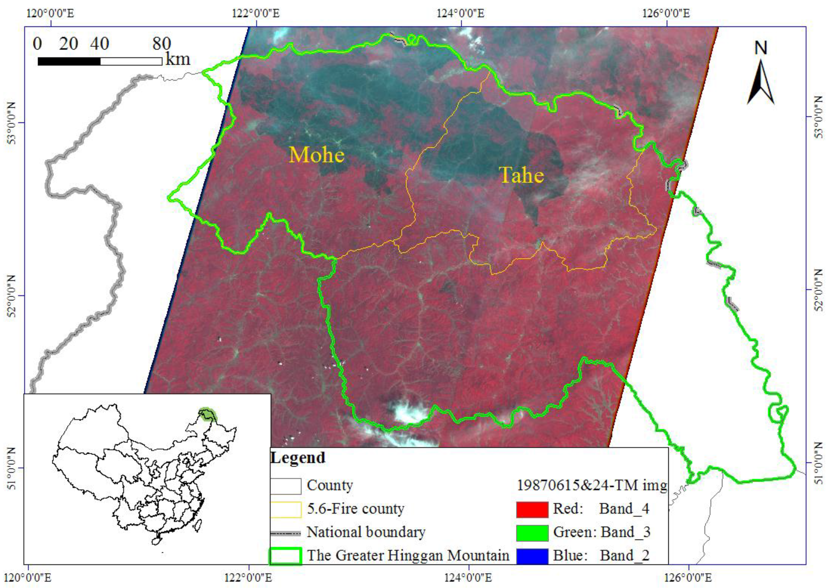
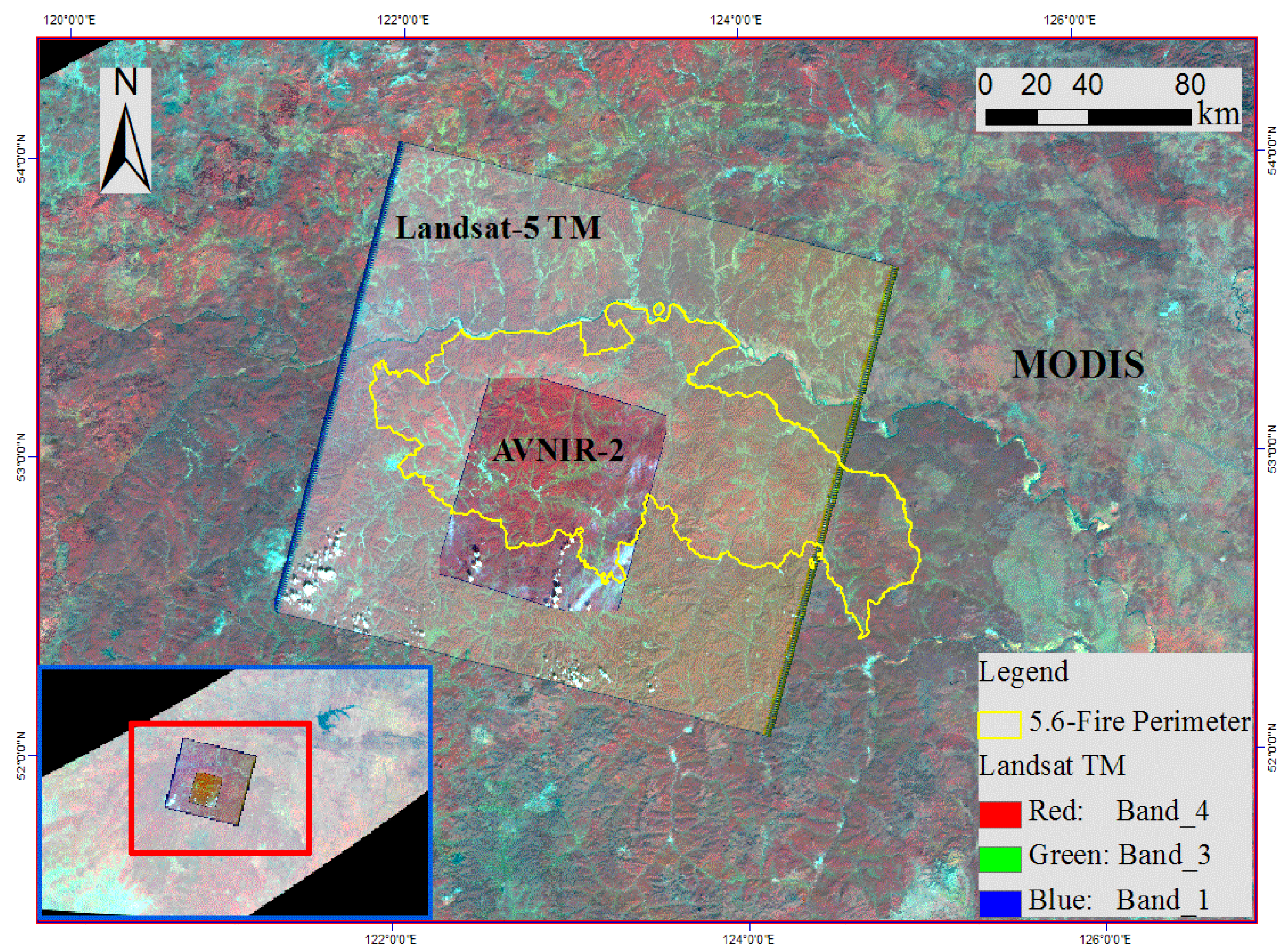
2.1. Study Area
2.2. Remote-Sensing Data
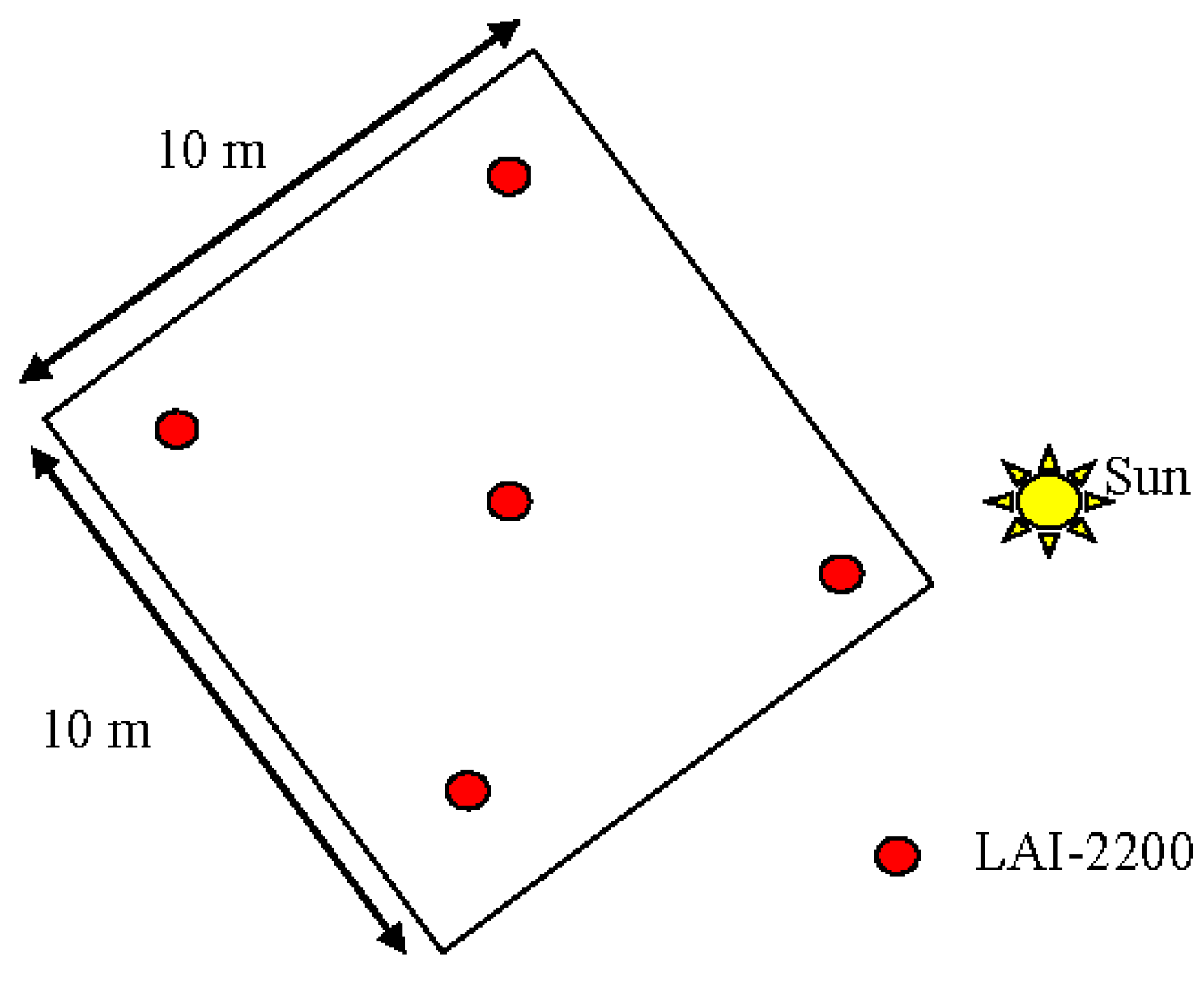
2.3. Field LAI Measurements
2.4. Data Pre-Processing
2.5. Multivariate Selection and Calculation
3. Results
3.1. Univariate Modeling Using Optical VIs
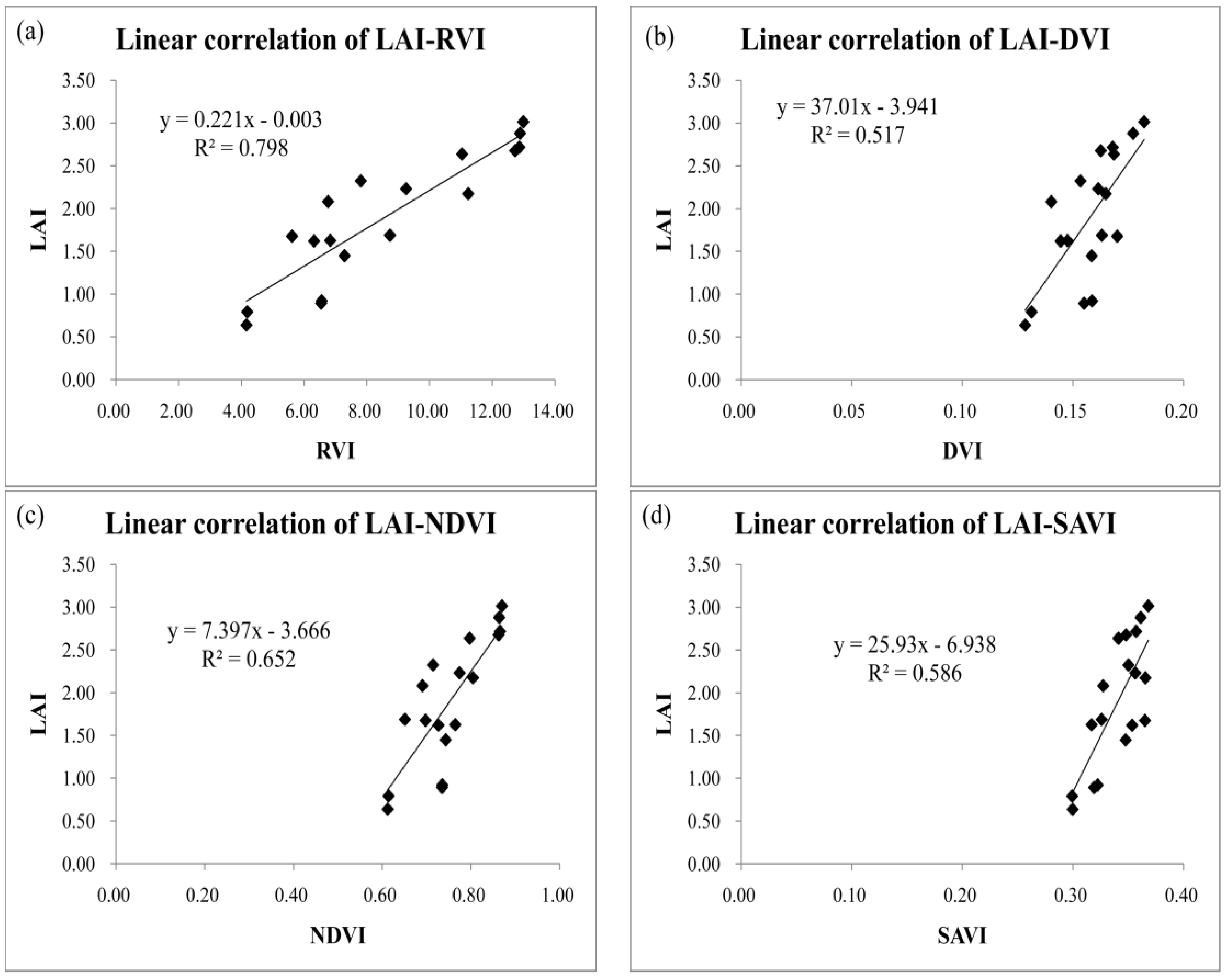
3.1.1. ALOS AVNIR-2 Data
3.1.2. Landsat-5 TM Data
3.1.3. MODIS NBAR Data
3.2. Multiple-Variable-Based Modeling
3.3. Comparison of Correlation between VIs
3.4. Comparison with PALSAR Indices
4. Discussion
4.1. Sensor Features and Statistical Modeling Evaluation
4.2. Future-Oriented Points for Improvements
5. Conclusions
Acknowledgments
Author Contributions
Conflicts of Interest
References
- Tucker, C.J.; Grant, D.M.; Dykstra, J.D. NASA’s global orthorectified Landsat data set. Photogramm. Eng. Remote Sens. 2004, 70, 313–322. [Google Scholar] [CrossRef]
- Wu, J.A.; Peng, D.L. Tree-Crown Information Extraction of Farmland Returned to Forests Using QuickBird Image Based on Object-Oriented Approach. Spectrosc. Spectr. Anal. 2010, 30, 2533–2536. [Google Scholar]
- Bontemps, S.; Langner, A.; Defourny, P. Monitoring forest changes in Borneo on a yearly basis by an object-based change detection algorithm using SPOT-VEGETATION time series. Int. J. Remote Sens. 2012, 33, 4673–4699. [Google Scholar] [CrossRef]
- Watanabe, M.; Shimada, M.; Rosenqvist, A.; Tadono, T.; Matsuoka, M.; Romshoo, S.A.; Ohta, K.; Furuta, R.; Nakamura, K.; Moriyama, T. Forest structure dependency of the relation between L-band sigma0 and biophysical parameters. IEEE Trans. Geosci. Remote 2006, 44, 3154–3165. [Google Scholar] [CrossRef]
- Liang, S.L. Quantitative Remote Sensing of Land Surfaces; John Wiley & Sons, Inc.: Hoboken, NJ, USA, 2004; pp. 1–10. [Google Scholar]
- Rastmanesh, F.; Moore, F.; Kharrati-Kopaei, M.; Behrouz, M. Monitoring deterioration of vegetation cover in the vicinity of smelting industry, using statistical methods and TM and ETM+ imageries, Sarcheshmeh copper complex, Central Iran. Environ. Monit. Assess. 2010, 163, 397–410. [Google Scholar] [CrossRef] [PubMed]
- Arias, D.; Calvo-Alvarado, J.; Dohrenbusch, A. Calibration of LAI-2000 to estimate leaf area index (LAI) and assessment of its relationship with stand productivity in six native and introduced tree species in Costa Rica. For. Ecol. Manag. 2007, 247, 185–193. [Google Scholar] [CrossRef]
- Chen, J.M.; Black, T.A. Defining leaf-area index for non-flat leaves. Plant Cell Environ. 1992, 15, 421–429. [Google Scholar] [CrossRef]
- Chen, W.; Cao, C.X.; He, Q.S.; Guo, H.D.; Zhang, H.; Li, R.Q.; Zheng, S.; Xu, M.; Gao, M.X.; Zhao, J.; et al. Quantitative estimation of the shrub canopy LAI from atmosphere-corrected HJ-1 CCD data in Mu Us Sandland. Sci. China Earth Sci. 2010, 53, 26–33. [Google Scholar] [CrossRef]
- Schleppi, P.; Thimonier, A.; Walthert, L. Estimating leaf area index of mature temperate forests using regressions on site and vegetation data. For. Ecol. Manag. 2011, 261, 601–610. [Google Scholar] [CrossRef]
- Chen, W.; Moriya, K.; Sakai, T.; Koyama, L.; Cao, C.X. Post-fire forest regeneration under different restoration treatments in the Greater Hinggan Mountain area of China. Ecol. Eng. 2014, 70, 304–311. [Google Scholar] [CrossRef]
- Guo, N. Vegetation index and its advances. J. Arid Meteorol. 2003, 21, 71–75. [Google Scholar]
- Sharma, R.C.; Kajiwara, K.; Honda, Y. Estimation of forest canopy structural parameters using kernel-driven bi–directional reflectance model based multi-angular vegetation indices. ISPRS J. Photogramm. 2013, 78, 50–57. [Google Scholar] [CrossRef]
- Chen, J.M.; Cihlar, J. Retrieving leaf area index of boreal conifer forests using Landsat TM images. Remote Sens. Environ. 1996, 55, 153–162. [Google Scholar] [CrossRef]
- Chen, W.; Moriya, K.; Sakai, T.; Koyama, L.; Cao, C.X. Monitoring of post-fire forest recovery under different restoration modes based on time series Landsat data. Eur. J. Remote Sens. 2014, 47, 153–168. [Google Scholar] [CrossRef]
- Xu, M.; Cao, C.X.; Tong, Q.X.; Li, Z.Y.; Zhang, H.; He, Q.S.; Gao, M.X.; Zhao, J.; Zheng, S.; Chen, W.; et al. Remote sensing based shrub above-ground biomass and carbon storage mapping in Mu Us desert, China. Sci. China Technol. Sci. 2010, 53, 176–183. [Google Scholar] [CrossRef]
- Arroyo, L.A.; Johansen, K.; Armston, J.; Phinn, S. Integration of LiDAR and QuickBird imagery for mapping riparian biophysical parameters and land cover types in Australian tropical savannas. For. Ecol. Manag. 2010, 259, 598–606. [Google Scholar] [CrossRef]
- Andersen, H.E.; Strunk, J.; Temesgen, H.; Atwood, D.; Winterberger, K. Using multilevel remote sensing and ground data to estimate forest biomass resources in remote regions: A case study in the boreal forests of interior Alaska. Can. J. Remote Sens. 2011, 37, 596–611. [Google Scholar] [CrossRef]
- Chen, X.; Vierling, L.; Deering, D.; Conley, A. Monitoring boreal forest leaf area index across a Siberian burn chronosequence: A MODIS validation study. Int. J. Remote Sens. 2005, 26, 5433–5451. [Google Scholar] [CrossRef]
- Chowdhury, T.A.; Thiel, C.; Schmullius, C.; Stelmaszczuk-Gorska, M. Polarimetric Parameters for Growing Stock Volume Estimation Using ALOS PALSAR L-Band Data over Siberian Forests. Remote Sens. 2013, 5, 5725–5756. [Google Scholar] [CrossRef]
- Han, N.; Du, H.Q.; Zhou, G.M.; Xu, X.J.; Cui, R.R.; Gu, C.Y. Spatiotemporal heterogeneity of Moso bamboo aboveground carbon storage with Landsat Thematic Mapper images: A case study from Anji County, China. Int. J. Remote Sens. 2013, 34, 4917–4932. [Google Scholar] [CrossRef]
- Schroeder, T.A.; Wulder, M.A.; Healey, S.P.; Moisen, G.G. Detecting post-fire salvage logging from Landsat change maps and national fire survey data. Remote Sens. Environ. 2012, 122, 166–174. [Google Scholar] [CrossRef]
- Millin-Chalabi, G.; McMorrow, J.; Agnew, C. Detecting a moorland wildfire scar in the Peak District, UK, using synthetic aperture radar from ERS-2 and Envisat ASAR. Int. J. Remote Sens. 2014, 35, 54–69. [Google Scholar] [CrossRef]
- Pearson, R.L.; Miller, L.D. Remote Mapping of Standing Crop Biomass for Estimation of the Productivity of the Shortgrass Prairie. In Proceedings of the Eighth International Symposium on Remote Sensing of Environment, Ann Arbor, MI, USA, 2–6 October 1972; Willow Run Laboratories, Environmental Research Institute of Michigan: Ypsilanti, Michigan, 1972; pp. 1355–1381. [Google Scholar]
- Jordan, C.F. Derivation of leaf area index from quality of light on the forest floor. Ecology 1969, 50, 663–666. [Google Scholar] [CrossRef]
- Rouse, J.W.; Haas, R.H.; Schell, J.A.; Deering, D.W. Monitoring Vegetation Systems in the Great Plains with ERTS. In Proceedings of the Third Earth Resources Technology Satellite-1 Symposium, Washington, DC, USA, 10–14 December 1973; NASA/GSFC: Greenbelt, MD, USA, 1974; pp. 309–317. [Google Scholar]
- Huete, A.R. A soil-adjusted vegetation index (SAVI). Remote Sens. Environ. 1988, 25, 295–309. [Google Scholar] [CrossRef]
- Kaufman, Y.J.; Tanre, D. Atmospherically resistant vegetation index (ARVI) for EOS-MODIS. IEEE Trans. Geosci. Remote 1992, 30, 261–270. [Google Scholar] [CrossRef]
- Liu, H.Q.; Huete, A.R. A feedback based modification of the NDVI to minimize canopy background and atmosphere noise. IEEE Trans. Geosci. Remote 1995, 33, 457–465. [Google Scholar]
- Haenlein, M.; Kaplan, A.M. A Beginner’s Guide to Partial Least Squares Analysis. Underst. Stat. 2004, 3, 283–297. [Google Scholar] [CrossRef]
- Tian, Y.H.; Wang, Y.J.; Zhang, Y.; Knyazikhin, Y.; Bogaert, J.; Myneni, R.B. Radiative transfer based scaling of LAI retrievals from reflectance data of different resolutions. Remote Sens. Environ. 2003, 84, 143–159. [Google Scholar] [CrossRef]
- Fan, W.J.; Gai, Y.Y.; Xu, X.R.; Yan, B.Y. The spatial scaling effect of the discrete-canopy effective leaf area index retrieved by remote sensing. Sci. China Earth Sci. 2013, 56, 1548–1554. [Google Scholar] [CrossRef]
- Zheng, G.; Moskal, L.M. Retrieving Leaf Area Index (LAI) Using Remote Sensing: Theories, Methods and Sensors. Sensors 2009, 9, 2719–2745. [Google Scholar] [CrossRef] [PubMed]
- Mitchard, E.T.A.; Saatchi, S.S.; Woodhouse, I.H.; Nangendo, G.; Ribeiro, N.S.; Williams, M.; Ryan, C.M.; Lewis, S.L.; Feldpausch, T.R.; Meir, P. Using satellite radar backscatter to predict above-ground woody biomass: A consistent relationship across four different African landscapes. Geophys. Res. Lett. 2009, 36, L23401. [Google Scholar] [CrossRef]
- Kobayashi, S.; Widyorini, R.; Kawai, S.; Omura, Y.; Sanga-Ngoie, K.; Supriadi, B. Backscattering characteristics of L-band polarimetric and optical satellite imagery over planted acacia forests in Sumatra, Indonesia. J. Appl. Remote Sens. 2012, 6, 063525. [Google Scholar]
- Suzuki, R.; Kim, Y.; Ishii, R. Sensitivity of the backscatter intensity of ALOS/PALSAR to the above-ground biomass and other biophysical parameters of boreal forest in Alaska. Polar Sci. 2013, 7, 100–112. [Google Scholar] [CrossRef]


| Satellite | Sensor | Bands | Wavelength Range (µm) | Spatial Resolution (m) | Swath Width (km) | Repeat Cycle (days) |
|---|---|---|---|---|---|---|
| ALOS | AVNIR-2 | 1 | 0.42–0.50 | 10 (at Nadir) | 70 (at Nadir) | 46 |
| 2 | 0.52–0.60 | |||||
| 3 | 0.61–0.69 | |||||
| 4 | 0.76–0.89 | |||||
| Landsat-5 | TM | 1 | 0.45–0.52 | 30 | 185 | 16 |
| 2 | 0.52–0.60 | |||||
| 3 | 0.63–0.69 | |||||
| 4 | 0.76–0.90 | |||||
| 5 | 1.55–1.75 | |||||
| 6 | 10.4–12.5 | 120 | ||||
| 7 | 2.08–2.35 | 30 | ||||
| Terra/Aqua | MODIS | 1 | 0.620–0.670 | 250 | 2330 (cross track) | 1-2 |
| 2 | 0.841–0.876 | |||||
| 3 | 0.459–0.479 | 500 | ||||
| 4 | 0.545–0.565 | |||||
| 5 | 1.230–1.250 | |||||
| 6 | 1.628–1.652 | |||||
| 7 | 2.105–2.155 |
| Mode | Fine | ScanSAR | Polarimetric | ||
|---|---|---|---|---|---|
| FBS | FBD | ||||
| Chirp bandwidth | 28 MHz | 14 MHz | 14 MHz, 28 MHz | 14 MHz | |
| Polarization | HH or VV | HH+HV or VV+VH | HH or VV | HH+HV+VH+VV | |
| Incident angle | 8–60 deg. | 8–60 deg. | 18–43 deg. | 8–30 deg. | |
| Resolution | Range | 7–44 m | 14–88 m | 100 m | 24–89 m |
| Azimuth | 10 m (2 looks) | 100 m | 10 m (2 looks) | ||
| 20 m (4 looks) | 20 m (4 looks) | ||||
| Swath width | 40–70 km | 40–70 km | 250–350 km | 20–65 km | |
| Bit length | 5 bits | 5 bits | 5 bits | 3 or 5 bits | |
| Data rate | 240 Mbps | 240 Mbps | 120 or 240 Mbps | 240 Mbps | |
| Center frequency | 1270 MHz (L-band) | ||||
| Radiometric accuracy | scene: 1 dB/orbit: 1.5 dB | ||||
| Independent Variables a | R | R2 | SEE b | F Statistics | Sig. |
|---|---|---|---|---|---|
| (a) ALOS AVNIR-2 | |||||
| RVI | 0.893 | 0.798 | 0.349 | 63.318 | 0.000 ** |
| DVI | 0.720 | 0.517 | 0.539 | 17.186 | 0.001 ** |
| NDVI | 0.808 | 0.652 | 0.458 | 29.987 | 0.000 ** |
| SAVI | 0.766 | 0.586 | 0.499 | 22.733 | 0.000 ** |
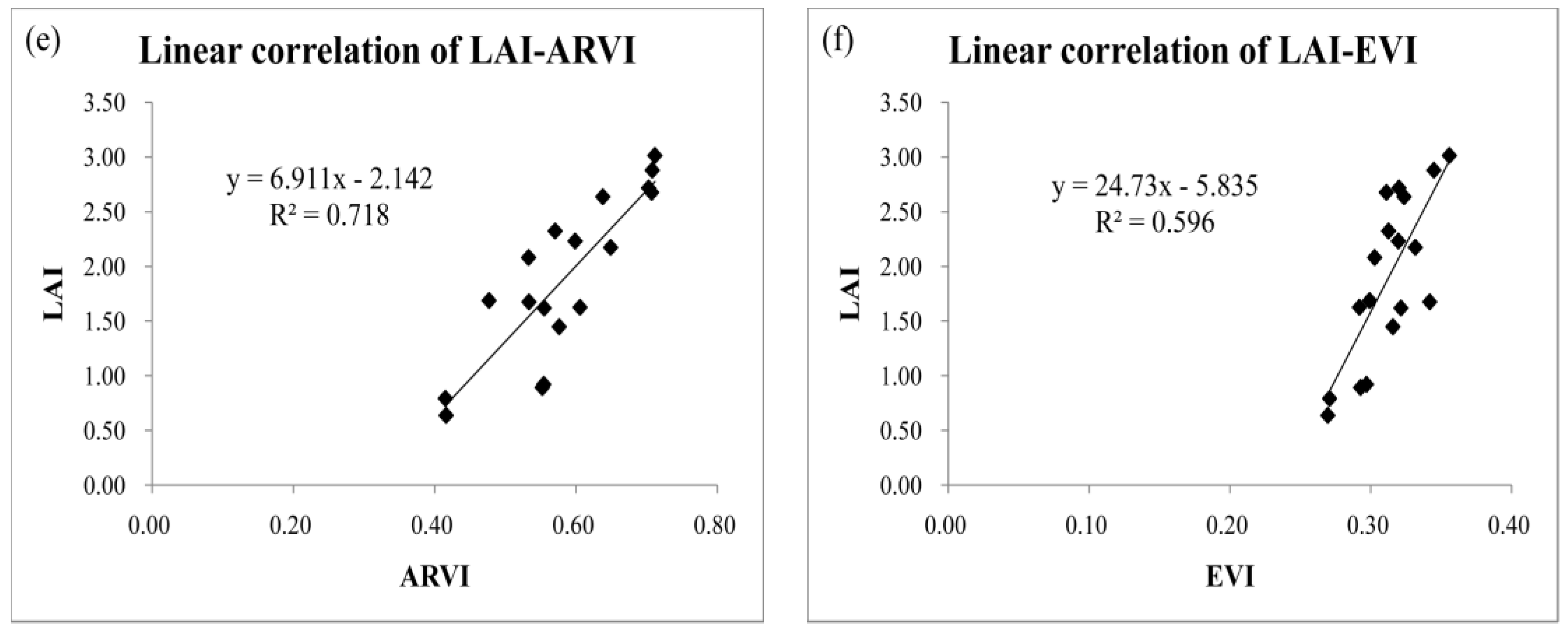
| ARVI | 0.848 | 0.718 | 0.412 | 40.853 | 0.000 ** |
| EVI | 0.773 | 0.596 | 0.493 | 23.685 | 0.000 ** |
| (b) Landsat-5 TM | |||||
| RVI | 0.823 | 0.677 | 0.441 | 33.585 | 0.000 ** |
| DVI | 0.625 | 0.391 | 0.606 | 10.279 | 0.006 ** |
| NDVI | 0.750 | 0.562 | 0.513 | 20.567 | 0.000 ** |
| SAVI | 0.693 | 0.480 | 0.560 | 14.783 | 0.001 ** |
| ARVI | 0.756 | 0.570 | 0.509 | 21.281 | 0.000 ** |
| EVI | 0.702 | 0.493 | 0.553 | 15.538 | 0.001 ** |
| (c) MODIS NBAR | |||||
| RVI | 0.687 | 0.471 | 0.518 | 8.920 | 0.014 * |
| DVI | 0.578 | 0.334 | 0.582 | 5.019 | 0.049 * |
| NDVI | 0.664 | 0.440 | 0.533 | 7.879 | 0.019 * |
| SAVI | 0.591 | 0.349 | 0.575 | 5.373 | 0.043 * |
| ARVI | 0.668 | 0.446 | 0.531 | 8.051 | 0.018 * |
| EVI | 0.644 | 0.415 | 0.545 | 7.094 | 0.024 * |
| (d) ALOS PALSAR | |||||
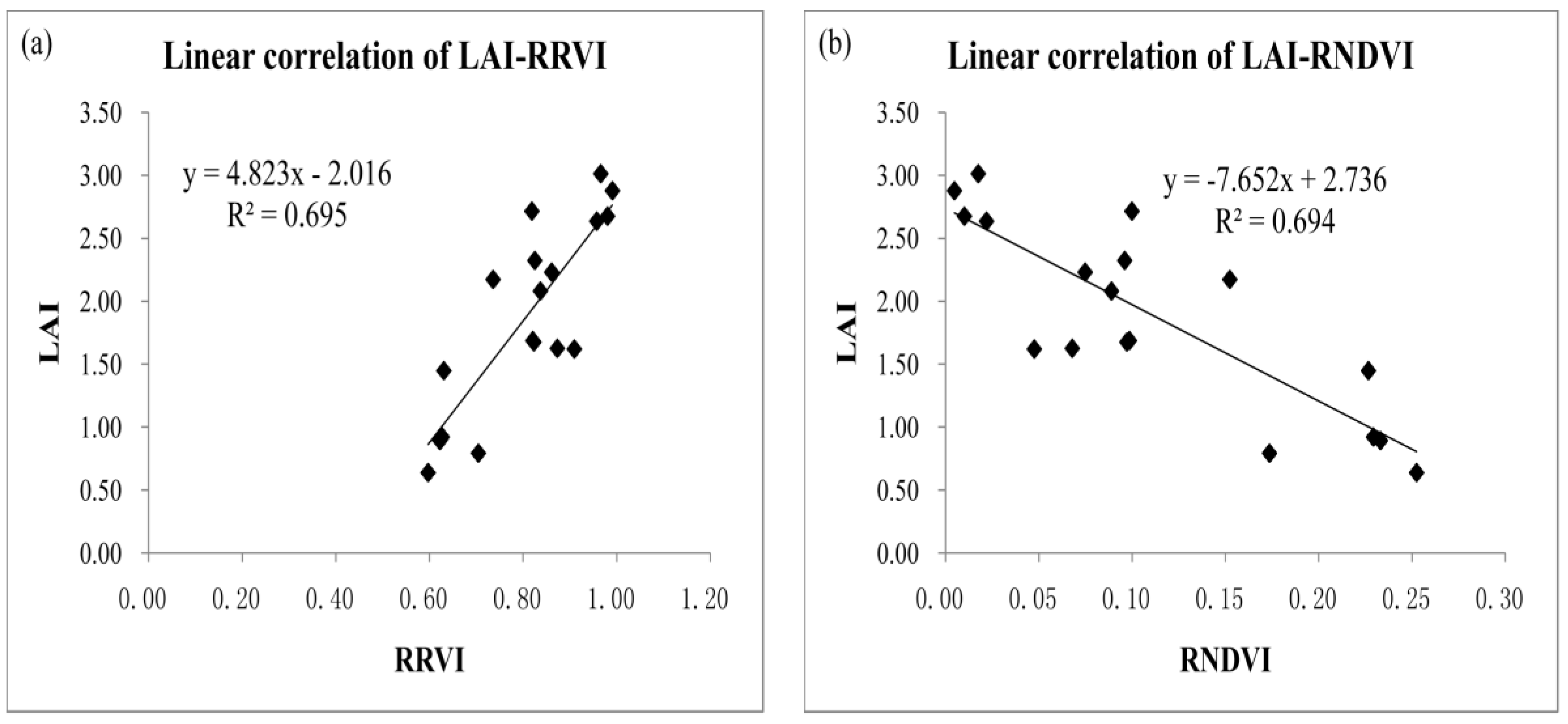
| RRVI | 0.834 | 0.695 | 0.429 | 36.465 | 0.000 ** |
| RNDVI | 0.833 | 0.694 | 0.429 | 36.380 | 0.000 ** |
| Sensors | R | R2 | Optimal No. of Components | Sig. |
|---|---|---|---|---|
| ALOS AVNIR-2 | 0.968 | 0.937 | 4 | 0.000 ** |
| Landsat-5 TM | 0.889 | 0.790 | 3 | 0.000 ** |
| MODIS NBAR | 0.826 | 0.682 | 5 | 0.000 ** |
| Sensors | RVI/RRVI | DVI | NDVI/RNDVI | SAVI | ARVI | EVI |
|---|---|---|---|---|---|---|
| AVNIR-2 and TM | 0.819 ** | 0.678 ** | 0.826 ** | 0.716 ** | 0.791 ** | 0.674 ** |
| TM and MODIS | 0.353 * | 0.274 | 0.281 | 0.266 | 0.368 * | 0.208 |
| AVNIR-2 and MODIS | 0.218 | 0.108 | 0.165 | 0.111 | 0.206 | 0.118 |
| AVNIR-2 and PALSAR | 0.422 * | 0.335 * |
© 2017 by the authors. Licensee MDPI, Basel, Switzerland. This article is an open access article distributed under the terms and conditions of the Creative Commons Attribution (CC BY) license (http://creativecommons.org/licenses/by/4.0/).
Share and Cite
Chen, W.; Yin, H.; Moriya, K.; Sakai, T.; Cao, C. Retrieval and Comparison of Forest Leaf Area Index Based on Remote Sensing Data from AVNIR-2, Landsat-5 TM, MODIS, and PALSAR Sensors. ISPRS Int. J. Geo-Inf. 2017, 6, 179. https://0-doi-org.brum.beds.ac.uk/10.3390/ijgi6060179
Chen W, Yin H, Moriya K, Sakai T, Cao C. Retrieval and Comparison of Forest Leaf Area Index Based on Remote Sensing Data from AVNIR-2, Landsat-5 TM, MODIS, and PALSAR Sensors. ISPRS International Journal of Geo-Information. 2017; 6(6):179. https://0-doi-org.brum.beds.ac.uk/10.3390/ijgi6060179
Chicago/Turabian StyleChen, Wei, Hang Yin, Kazuyuki Moriya, Tetsuro Sakai, and Chunxiang Cao. 2017. "Retrieval and Comparison of Forest Leaf Area Index Based on Remote Sensing Data from AVNIR-2, Landsat-5 TM, MODIS, and PALSAR Sensors" ISPRS International Journal of Geo-Information 6, no. 6: 179. https://0-doi-org.brum.beds.ac.uk/10.3390/ijgi6060179