
SCMDOT: Spatial Clustering with Multiple Density-Ordered Trees

Key Laboratory of Spatial Data Mining & Information Sharing, Ministry of Education, Fuzhou University, Fuzhou 350002, China
*
Author to whom correspondence should be addressed.
ISPRS Int. J. Geo-Inf. 2017, 6(7), 217; https://0-doi-org.brum.beds.ac.uk/10.3390/ijgi6070217
Submission received: 21 May 2017
/
Revised: 8 July 2017
/
Accepted: 10 July 2017
/
Published: 13 July 2017
Abstract
:With the rapid explosion of information based on location, spatial clustering plays an increasingly significant role in this day and age as an important technique in geographical data analysis. Most existing spatial clustering algorithms are limited by complicated spatial patterns, which have difficulty in discovering clusters with arbitrary shapes and uneven density. In order to overcome such limitations, we propose a novel clustering method called Spatial Clustering with Multiple Density-Ordered Trees (SCMDOT). Motivated by the idea of the Density-Ordered Tree (DOT), we firstly represent the original dataset by the means of constructing Multiple Density-Ordered Trees (MDOT). In the constructing process, we impose additional constraints to control the growth of each Density-Ordered Tree, ensuring that they all have high spatial similarity. Furthermore, a series of MDOT can be successively generated from regions of sparse areas to the dense areas, where each Density-Ordered Tree, also treated as a sub-tree, represents a cluster. In the merging process, the final clusters are obtained by repeatedly merging a suitable pair of clusters until they satisfy the expected clustering result. In addition, a heuristic strategy is applied during the process of our algorithm for suitability for special applications. The experiments on synthetic and real-world spatial databases are utilised to demonstrate the performance of our proposed method.
1. Introduction
Spatial data mining has been emphasised for a decade in an effort to discover potential and meaningful knowledge hidden in the intensely massive numbers of spatial objects. Spatial clustering is one of the most significant branches of spatial data mining, which aims to classify numerous of spatial objects with diverse spatial distribution into several groups (called clusters). Briefly, the principle of spatial clustering is to ensure that spatial objects are sorted in the same cluster with a higher spatial similarity compared to those belonging to other clusters. The natural spatial agglomeration patterns from spatial objects can be completely revealed by analysis of spatial clustering. Spatial clustering has been widely applied in various fields of real life, such as climate change, crime hotspot analysis, disease surveillance, seismic investigation and so on [1,2,3,4].
Nowadays, with the sharp expansion and update of modern spatial databases, a growing number of complicated and diverse spatial patterns are developed, which has posed a big challenge for the existing spatial clustering techniques. Due to some drawbacks of traditional spatial clustering algorithms as they are based upon relatively static models, they do not have the ability to effectively handle the increasingly tricky problems, such as density problem, shape problem and touching problem [5]. Specifically, spatial objects with mixed densities in addition to clusters with arbitrary shapes and diverse spatial relations may lead clustering method to obtain unqualified and unstable results in some cases.
To the best of our knowledge, a large amount of existing clustering approaches have been proposed in the literature [6,7], which can be roughly grouped into partitional clustering, hierarchical clustering, density-based clustering, grid-based clustering, graph-based clustering and model-based clustering. However, most of these approaches are vulnerable to the different cluster sizes, shapes and densities. K-means [8], a widely employed partitional clustering method, is susceptible to noises and prefers to detect clusters of spherical shape, which derives from its specific criterion of division. Density Based Spatial Clustering of Applications with Noise (DBSCAN) [9] is the pioneer of the density-based clustering method. Although it is able to discover clusters of arbitrary shapes, the uncertainty of tuning the input parameters makes it unable to deal with unbalanced density of different clusters. The affinity propagation algorithm (AP) [10] presents a simple and efficient way to find out the collection of most suitable points representing clusters by repeatedly transmitting real-valued messages between data points, although it is still limited in identifying the clusters with various shapes.
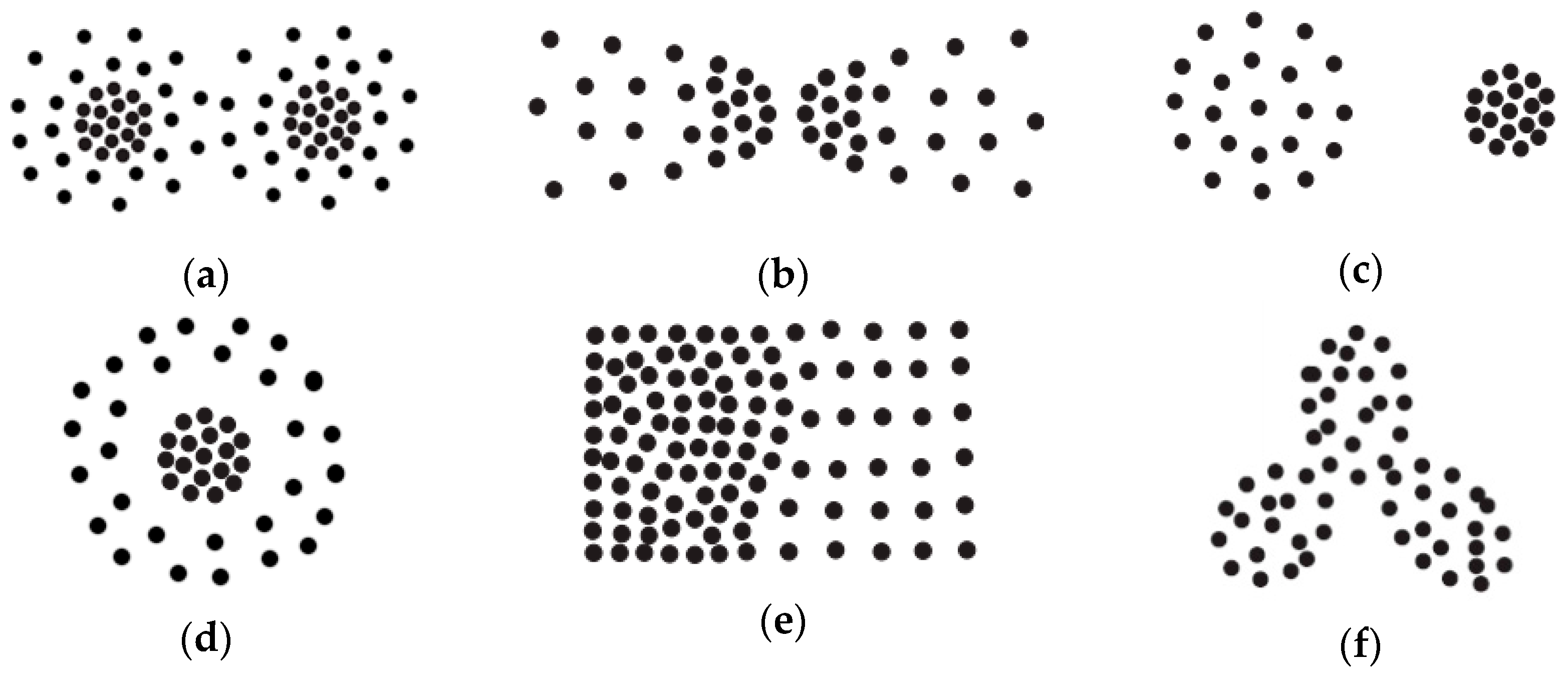
For the purpose of having an intuitive understanding of these challenges, some representative spatial patterns are shown in Figure 1, which includes clusters with different shapes, sizes and densities.
Inspired by the idea of Spatial Clustering with Density-Ordered Tree (SCDOT) algorithm [11], we put forward a novel clustering method in this paper, which is called Spatial Clustering with Multiple Density-Ordered Trees (SCMDOT). This method is proposed to handle complex and inhomogeneous spatial patterns. SCMDOT unites the advantages of hierarchical clustering, density-based clustering and graph-based clustering. Both the distance and density are simultaneously taken into account for clustering. In addition, a heuristic strategy is utilised to optimise the clustering results and be suitable for special applications, which runs through the process of our algorithm. While there are benefits from the mixed ideas of clustering, our method can be adapted to detect the variations in density in a hierarchical way and improve the accuracy of clustering by building graph models. This provides a useful fashion to not only discover clusters with arbitrary shapes, but also identify spatial objects with multi-densities.
The main contributions of this paper can be summarised as follows:
- We propose an innovative method to represent a dataset by constructing a series of constrained Multiple Density-Ordered Trees (MDOT) in the proper order. During the process of generating MDOT, a high spatial similarity of each cluster can be ensured. In this way, our algorithm is capable of not only handling the problem of separating clusters with complex structures, but also increasing the robustness and reliability of the clustering result.
- Our method introduces a novel approach based on MDOT to identify noises and cluster centres. Noises which included in the inappropriate start points before constructing MDOT and can be further confirmed rely on the deviation from the final clusters. In addition, cluster centres can be recognised as the roots of MDOT.
- The proposed method can be adapted to the detection of clusters with different shapes and uneven density, which has been especially proved effective in the case of adjacent clusters with distinctly varied densities.
The rest of the paper is organised as follows. In Section 2, we will review the clustering with the density peaks proposed recently, classical graph-based clustering methods and SCDOT algorithm. The SCMDOT algorithm we propose will be described in detail in Section 3. The experiments on synthetic and real databases are shown in Section 4. Finally, conclusions are made and future work is discussed in Section 5.
2. Related Works
The goal of performing adaptive spatial clustering mainly depends on two essential requirements. One is the ability to effectively and efficiently identify and handle the density variation in spatial patterns, while the other one is discovering clusters with irregular structures under the precondition of ensuring the similarity between spatial objects.
Most existing clustering methods hardly meet both the above requirements at the same time, which are limited by their own fixed clustering schemes. Recently, a novel clustering approach, which is called clustering by fast search and find of density peaks (CFSFDP) [12], was proposed by Rodriguez and Laio, which creatively uses a combination of density and distance as the measure in judging the similarity between data points. The algorithm has its basis in the assumptions that cluster centres are characterised by a higher density than their neighbours and by a relatively large distance from points with higher local densities. The local density of each data point () and the distance from data point to its nearest neighbour with a higher density () are calculated during the process of CFSFDP. Based on a given cut-off distance () employed to determine the local density of data points and identify border points of each cluster, CFSFDP can quickly and simply find clusters with varied densities and arbitrary shapes. Compared with DBSCAN, it provides an efficient way of assigning data points to clusters by using the idea of density peaks, which can effectively distinguish clusters and remove noises. Meanwhile, it requires less parameters and has a lower time complexity for its non-iteration (with a time complexity of O(N), where N is the number of objects). However, there are still some weaknesses of CFSFDP, which are as follows: (1) The calculation of , a major limitation of CFSFDP, heavily depends on the prior knowledge, which is too difficult to estimate. The sensitivity of choosing has a great effect on the final clustering results. (2) It is tough for users to select suitable cluster centres by plotting a decision graph in some complicated cases. (3) If a cluster contains more than one density peak, CFSFDP is unable to address the issue well. Aiming at improving the defects mentioned above, Mehmood [13] presented a method called CFSFDP via heat diffusion (CFSFDP-HD), which involves enhancement of the accuracy of densities of data points based on the heat diffusion to reduce the demands of setting the sensitive cut-off parameter (). However, it still requires users to subjectively choose cluster centres. Xu et al. [14] proposed a density peak based hierarchical clustering method (DenPEHC), which generates clusters directly on each possible clustering layer and introduces a grid granulation framework to enable DenPEHC to cluster large-scale and high-dimensional (LSHD) datasets.
In addition, in order to express the relationship between data points in an intuitive way and take it as the basis of similarity measurements, a graph is undoubtedly a useful method to reveal the structure of a spatial dataset. Actually, graph-based clustering [15] takes advantage of graph concepts to represent a dataset where the node is regarded as the data point and the edge is regarded as the relationship among data points. The typical methods for clustering based upon the graph include graph clustering using k nearest neighbours and minimum spanning tree (MST)-based clustering, which are commonly used as the solid foundation of related research. CHAMELEON [16] is a representative graph clustering algorithm using k nearest neighbours. The algorithm allows for analysis of the dataset in two phases. In the first phase, it effectively partitions the k nearest neighbours and graphs into many small sub-clusters by minimizing the edge-cut. During the next phase, the agglomerative hierarchical clustering algorithm is applied to merge these sub-clusters into final clusters. Both the relative inter-connectivity and relative closeness are defined in the phase of merging. Therefore, it can consider both the inter-connectivity and the intra-similarity of clusters, which provides a dynamic model of merging clusters. Zahn [17] first proposed MST-based clustering. Due to MST-based clustering methods representing a dataset by constructing the minimum spanning tree, its main idea is in accordance with the principle of clustering to a great extent. The criteria for identifying different clusters utilises the notion of a scale. While detecting clusters from a multi-scale, it is effective in perceiving and discovering some inconsistent edges (e.g., edges corresponding to maximum weights), which are abnormal compared to other edges in the same cluster. As a matter of fact, the separation of clusters by removing these inconsistent edges is valid in some specific structures. However, traditional MST-based clustering algorithms may not be useful when clustering in complex situations. Essentially, in the case of the inhomogeneous distribution, the discernment of inconsistent edges is very difficult and thus, it is unreliable to distinguish the separation of clusters. Some improved clustering algorithms based on MST, such as two rounds of MST (2-MSTClus) [18] and minimum spanning tree based split-and-merge method (SAM) [19], have been proposed in order to alleviate these deficiencies. 2-MSTClus divides the problem into two groups composed of separated cluster problems and touching cluster problems, which are two relatively independent schemes that are mutually complemented to solve tough clustering issues. SAM employs the split-and-merge strategy, which is intended to guide the splitting and merging process so as to capture the intrinsic structure of a dataset. Nevertheless, both of them have relatively static models and are not robust to noises.
Considering the superiority of the above spatial clustering theories, Cheng et al. [11] more recently developed a new method to have a great combination of both the idea of density peaks and the graph theory by the approach of constructing a Density-Ordered Tree (DOT). In the light of ideas related to density peaks, SCDOT can not only take into account both distance and density between data points but also efficiently obtain cluster centres and identify noises. In addition, inspired by graph clustering, the algorithm fully absorbs the advantages of spanning tree in creating strong links between the pairs of points contained in the graph. Similar to most effective hybrid strategies adopted by some hierarchical clustering methods, such as the agglomerative-and-divisive method, split-and-merge method and group-optimise method [20], SCDOT takes the split-and-merge strategy used in Chameleon and SAM in order to make the clustering analysis more reliable. This is related to the partition, hierarchical and density-based clustering principles. Indeed, SCDOT divides a whole DOT into many sub-clusters by using the box-plot method to reduce the influence of subjectively choosing cluster centres. Following this, SCDOT merges these sub-clusters by minimizing a measure. In the procedure of splitting DOT, SCDOT is capable of identifying noises and cluster centres from points contained in the inconsistent edges that were removed. Specifically, cluster centres are recognised as the roots of sub-trees, while noises are regarded as anomalous leaves. In general, SCDOT, a novel combinational clustering algorithm, provides an improved way to discover clusters with various shapes and densities more effectively. However, similar to most MST-based clustering algorithms, SCDOT unavoidably experiences the analogous dilemma, which is namely how to reasonably create the separation of clusters in some complex cases to more effectively meet the requirements of adaptive spatial clustering.
3. SCMDOT Algorithm
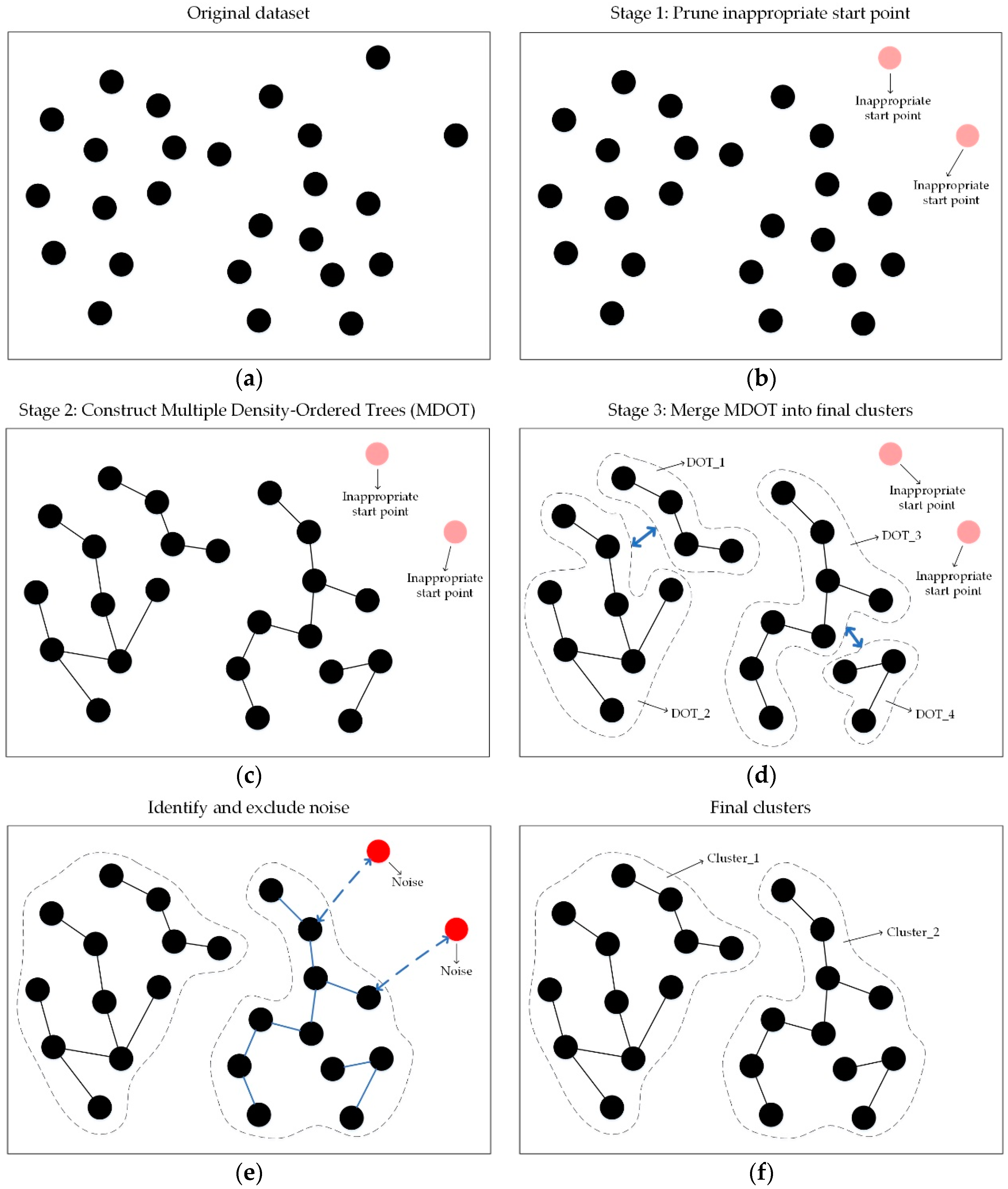
In this section, we will first list the limitations of the current study on SCDOT and explain the main causes of these issues. On this basis, we will introduce our novel spatial clustering algorithm in detail, which is called the Spatial Clustering with Multiple Density-Ordered Trees (SCMDOT). Furthermore, we will propose a new concept of MDOT for improving the insurmountable problems of SCDOT. In the implementation, SCMDOT is composed of three main stages as illustrated in Figure 2. In the first stage, the inappropriate start points are pruned to speed up the efficiency of the algorithm and improve the following construction of MDOT. In the stage of constructing, MDOT representing the original dataset are successively generated under certain constraints in order to guarantee a high spatial similarity for each cluster. In the stage of merging, the final clusters with different shapes and densities are obtained by comprehensive measurements of both the inter-connectivity and intra-similarity between clusters.
As mentioned in the previous section, SCDOT provides an effective and efficient way to facilitate clustering analysis. Nevertheless, some problems still exist when facing some complex datasets. First of all, when dealing with the adjacent clusters of varied densities, it is far from easy for SCDOT to find and remove the inconsistent edges, which will have a significant impact on dividing a whole Density-Ordered Tree into several sub-clusters. With regards to the above issue, it may result in some meaningless and invalid partitions instead of completely distinguishing clusters of diverse densities. Secondly, the spatial similarity of each cluster cannot be guaranteed by cutting DOT with an inflexible split strategy. Finally, the ignorance of the intra-similarity of clusters in the merging stage is another troublesome restriction of SCDOT, which means that it is possible for clusters with distinct similarities to be incorrectly merged into the same cluster. Thus, this could lead to unreasonable spatial clustering results.
According to the shortcomings mentioned above, we proposed the following methods to overcome these limitations for improving the quality of clustering results.
- We introduce an innovative way of developing a dynamic agglomerative model to represent the original dataset. Being different from the method employed by SCDOT, a series of clusters can be successively generated from regions of sparse areas to the dense areas rather than partitioning a whole DOT into several sub-clusters, which can circumvent the issues of splitting clusters.
- With the goal of ensuring a high spatial similarity for each cluster, we adopt a new tactic to control the growth of DOT in terms of edge growth and density change by imposing certain restrictions. From another point of view, the spatial similarity of each cluster will be guaranteed consistently during the procedure of construction.
- An improved criterion of merging clusters is proposed in this paper. Due to the improvement mentioned above providing an effective way to acquire internal proximity of each cluster, we are able to use it as an important indicator to measure the intra-similarity of clusters in the merging process so as to adapt to the change in local density among clusters.
3.1. Prune Inappropriate Start Points
Before the MDOT is constructed, the pruning stage of detecting and removing inappropriate start points is the prerequisite of the constructing stage, which aims to accelerate the process of algorithm and to minimise the impact on the following task. More specifically, too much time will be spent in handling the number of noises that exist in the spatial dataset. On the other hand, inappropriate start points have a negative effect on the growth of MDOT. Generally, it is a feasible choice to first remove these sensitive data points and later make further identification to determine whether they are noises or not.
In the process of the stage, we have to measure the dissimilarity between data points. Hence, the dissimilarity between data point i and j, denoted by , is defined in Equation (2). With the assumption that o is the data point belonging to the set of inappropriate start points, the identification criterion of an inappropriate start point is shown in Equation (3).
where represents the distance between data point i and j; denotes the number of nearest neighbours when constructing MDOT; represents nearest neighbours of data point i; and (a positive figure) is the threshold value for identification. A smaller value for means a more rigorous identification. Accordingly, more data points may be recognised as the inappropriate start points. In practice, is set to 1 by default in this paper.
For the sake of pruning inappropriate start points according to Equation (1), we attempt to seek out the point, which is considerably far away from its nearest neighbours. At the same time, the neighbours respectively have a relatively close distance to their nearest neighbours. In other words, when determining whether a data point is an inappropriate start point or not, there are two major aspects of judgment. The one is the deviation between data point and its neighbours, while the other one is the local density distribution of neighbours.
3.2. Construct Multiple Density-Ordered Trees (MDOT)
Let DB denote a spatial database of N spatial points and DB’ represent the pruned version of DB (DB with the inappropriate start points removed). The goal of clustering is to partition the set DB into K clusters C , where . A graph G(V, E) is constructed, where V is the set of points (also called nodes) in DB and E is the set of edges connecting pairs of vertices in V.
The local density of data point i is defined as the following equation:
Remark 1.
When calculating the local density of the data point i in DB’, we do not consider the other data point with the same spatial coordinates of i.
With the definition of local density mentioned above, the density order of data points can be expressed as follows:
One of the constraining factors, the Density Change Factor (DCF), is used to limit the density variation of the data point i in DB’ when constructing MDOT, which is represented as Equation (6). The threshold value of DCF is denoted as .
A graph of a sub-tree including n edges is denoted as ST; represents the set of the edges of ST, is the ith edge in E(ST) with representing the length of ; and E(ST) is defined as the expected edge in ST, which is the average of the edges in ST. This is represented as Equation (7).
Another constraining factor, Edge Growth Factor (EGF), is utilised to limit the growth of edges when constructing MDOT. Let ST represents a sub-tree including n edges. When adding a new edge into ST, denoted by , will change. Therefore, the Edge Growth Factor of is denoted by EGF(), which is represented as Equation (8). The threshold value of EGF is denoted as .
Remark 2.
During the process of constructing MDOT, if a sub-tree has not contained edges yet, we connect the sub-tree’s start point to its nearest point with a higher density under the constraints of DCF in DB’. Note that the point with the highest density is the start point in some exceptional cases. Essentially, if there are no points to connect with it, we assign the point to its nearest sub-tree.
Furthermore, the distance of point i is measured by computing the minimum distance between the point i and any other point with the higher density under double constraints, which is denoted as Equation (9). Based on the and , the threshold value of density variation of data point i is represented as , while the threshold value of edge growth of data point i is represented as .
Remark 3.
When searching the next connection point of data point i (excluding the start point of sub-tree) in DB’ during the constructing stage, we first find the suitable points under the constraints of the Density Change Factor (DCF), regarding them as candidate points. Following this, determine the most suitable connection point of data point i from these candidate points. Within the constraints of the Edge Growth Factor (EGF), the connection point is the one that has the nearest distance from its previous point in ST.
Remark 4.
For data point i, if the number of its next connection point(s) is more than one, we randomly choose one to connect it with.
Remark 5.
While the data point with the highest density is DB’, we conventionally take , so we do not need to connect it to any other data point if it is not the start point of the sub-tree.
Remark 6.
Each Density-Ordered Tree (DOT) has its unique density peak point (the point with the highest local density of sub-tree). We regard these density peak points of sub-trees as cluster centres.
According to the above definitions, we can assign each data point in DB’ to its next connection point and build a graph to link each pair of connection data points by making edges. The degree of link(s) is denoted as the weight of edge () in terms of Equation (9).
Furthermore, a heuristic strategy is adopted to choose critical parameters in this stage, which offers an exploratory way for obtaining specific clustering results. Although this requires relatively strict or loose conditions of clustering, the user can modify the threshold values of parameters to fit with special applications. However, it is necessary for us to give the recommended threshold values ( = 30%, = 40%), which is reasonable in order to ensure the reliability and consistency of the final cluster result.
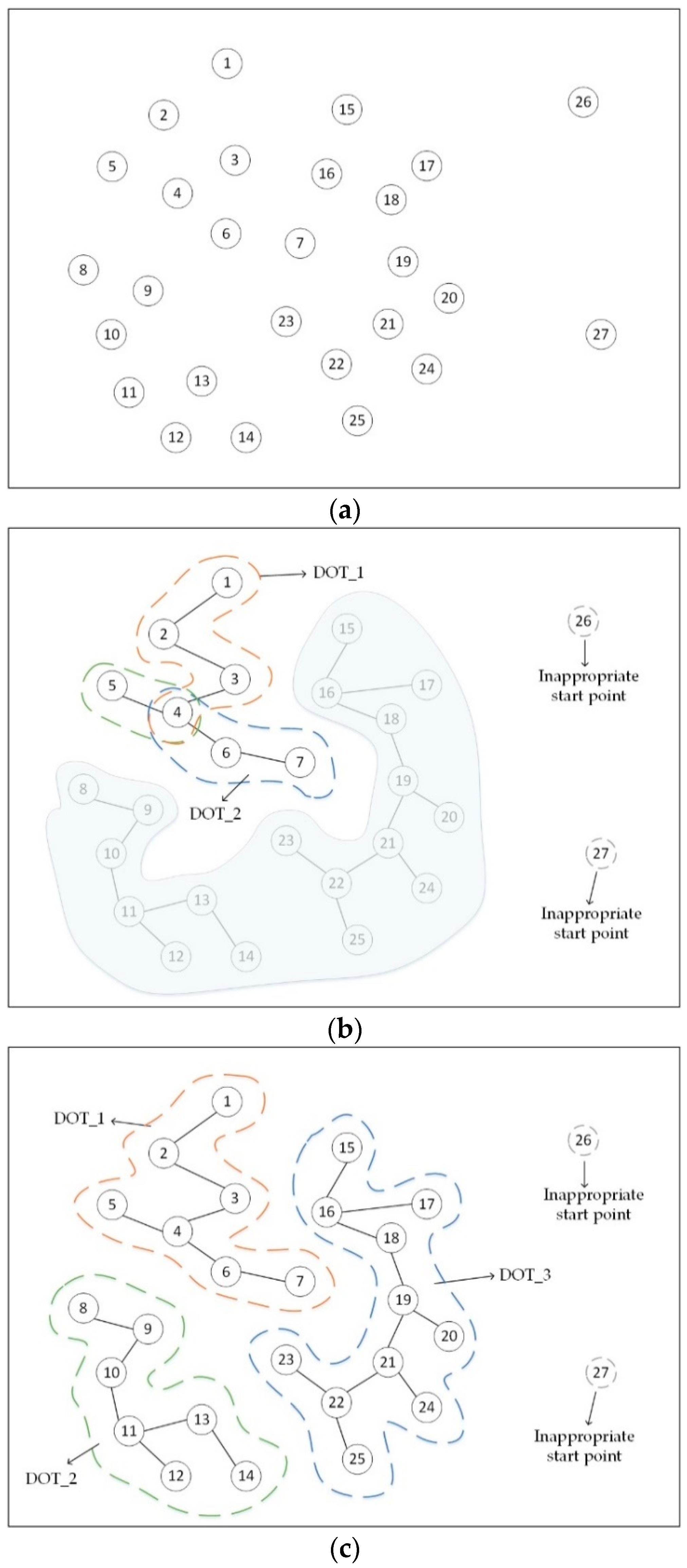
Figure 3 intuitively shows a simple example to illustrate the procedure of constructing MDOT (suppose that and point i is denoted as ). It is clear to see that and have been previously removed as the inappropriate start points. Since has the lowest local density of dataset, we select it as the initial start point. Based on the criteria of generating MDOT, we will successively connect and ; and ; and ; and stop at . Furthermore, we repeatedly choose the next suitable start point to generate a sub-tree and ultimately complete the whole construction of MDOT, as shown in Figure 3c. During the process of construction, MDOT grows constantly when adding in new members from other sub-trees. For instance, from Figure 3b, DOT_2 including , and adds into DOT_1 due to the connection between and . This means that DOT_1 and DOT_2 belong to the same cluster. Moreover, it is noteworthy to show that the effect of double constraints was imposed to control the growth of MDOT. In Figure 3c, although and is the nearest point from , we cannot connect to when . Instead, is the most suitable connection point of . Hence, DCF is a crucial factor to identify points with diverse densities. Furthermore, as displayed in Figure 3c, when and (4, 11) , cannot connect with . When limited by EGF, it is impossible to fall into the dilemma of splitting clusters.
3.3. Merge MDOT into Final Clusters
For enhancing the robust ability to find clusters of complex shapes and diverse densities, a great number of established MDOT are supposed to be merged while the total number of these sub-trees being larger than the target number (goal) of final expected clusters. In this phase, we introduce a new measure of merging clusters.
The measure of merging clusters will in fact be application-specific in the sense that it will depend on the intrinsic skeleton of the database being analysed. However, the vast majority of existing agglomerative schemes, such as CURE [21] and ROCK [22], rarely have a good combination of both inter-cluster similarity and intra-cluster closeness. In particular, the affinity between the data points in the same cluster has had less attention during the process of merging, which may lead to the incorrect merging of clusters in a similar way to the case in Figure 1e. On account of the relatively static agglomerative model of such schemes, it is subsequently impossible for the implementation of flexible merging decisions.
To overcome the limitations mentioned above, we propose a new notion according to Equations (10) and (11) to focus on measuring the intra-similarity of clusters with arbitrary shapes and non-homogeneous density. By taking advantage of the exclusive characteristics of MDOT, we can easily and effectively measure these.
For acquiring the internal proximity of each cluster, let denote the set of edges within ; is the number of edges in ; and belongs to , j . The internal proximity (IP) of is defined as follows:
Accordingly, the intra-similarity (IS) between and is given by:
The above definition is the part of overall merge index to measure the intra-cluster similarity of clusters. When there is a pair of clusters with a higher merge index, the internal proximity of these clusters will be closer.
In addition, another merging strategy proposed by Jong-Seok Lee [23,24] should be introduced in order to take the inter-connectivity between clusters into consideration. The criteria are required for measuring using the principles of clustering, namely the cluster k-Nearest Neighbour consistency (k-NN consistency) and the cluster k-Mutual Nearest-Neighbour consistency (k-MN consistency). In detail, if point i and its neighbour point j respectively belong to different clusters, a penalty will be imposed and the k-NN consistency of these clusters will reduce. Moreover, if point i also belongs to the neighbour of point j, the same penalty will be imposed and the k-MN consistency between these clusters will decrease. Motivated by this principle, a lower k-NN consistency and k-MN consistency of clusters is equivalent to a higher possibility of clusters to be merged. Hence, making better use of the principle will be conducive to the accurate measurement of inter-connectivity between clusters.
The overall merge index, called MergeValue, combines both the intra-similarity and inter-connectivity of different clusters. The MergeValue between and is denoted by MergeValue(), which is defined as follows:
where ; ; is the number of nearest neighbours when merging MDOT; represents nearest neighbours of data point i; denotes the number of data points in C; and represents the intra-similarity between cluster i and cluster j.
Regarding the measure proposed above, it is observed that MergeValue takes inter-connectivity and intra-similarity of clusters into account as a whole, while higher MergeValue between clusters implies that the pair of these clusters are prioritised for merging. Similar to the method by Cheng et al. [11], an iterative heuristic strategy is provided by automatically selecting parameters for obtaining the final expected clustering result. However, one of the key differences from SCDOT when merging clusters is that we use diverse parameters to define the number of nearest neighbours in the stage of constructing MDOT () and the merging stage (). In comparison with SCDOT utilizing only one parameter (k) to merge clusters in a heuristic way, there will be a lower computational cost due to avoiding the reconstruction of DOT. Furthermore, the intra-similarity of clusters has been particularly emphasised. Throughout the merging process, it can be summarised in the following four steps.
Step 1: Given initial k nearest neighbours () in the merging stage, calculate the MergeValue between clusters according to Equation (12).
Step 2: Find out the cluster merely owning few points and with an extremely low MergeValue relative to all other clusters. This cluster is not allowed into the following merging process.
Step 3: Rank pairs of clusters by MergeValue and choose the best pair with the highest MergeValue (MergeValue greater than 0) as the candidate to be merged for Step 4.
Step 4: Judge whether the number of clusters (K) is equal to the expected number of clusters (goal). If K = goal, the merging process stops and the final clusters are obtained. Otherwise, merge the pair of clusters selected in Step 3 and thus, the number of clusters decrease (. Following this, repeat Step 3 and Step 4.
It is worth to be noted that if the number of clusters does still not reach the target (goal) by repeatedly merging, will automatically update and then go through the merging process again in an iterative heuristic way.
Remark 7.
Considering that spatial databases are composed of the characteristics of the inhomogeneous distribution, it may be possible to generate clusters including only few points during the merging process. While some of these micro-clusters may have vastly lower MergeValues relative to all other clusters, this makes it difficult to be merged. To alleviate the influence above, we find out these clusters and do not allow them into merging. After the merging process has terminated, we respectively assign points contained in these micro-clusters to the cluster centre nearest to them and then remove these micro-clusters.
After reaching the goal of the desired number of clusters, the inappropriate start points removed previously in Section 3.1 are supposed to undergo further identification. The criterion of judgment relies on the deviation between the inappropriate start point and its nearest neighbour point contained in final clusters. In addition, with regards to a flexible cover range of final clusters, the internal proximity of each final cluster is defined as the maximal internal proximity of sub-trees that it contains. The inappropriate start point is recognised as noise only if the deviation is larger than the internal proximity of the corresponding final cluster. Otherwise, it will be distributed to the final clusters.
3.4. Algorithm and Performance Analysis
From the description in the previous sections, it can be seen that our algorithm mainly consists of three phases. The overall procedure of SCMDOT is summarised in Algorithm 1, while the stages of constructing and merging MDOT are respectively described in Algorithm 2 and Algorithm 3.
In Step 1, the matrix of data points in the spatial dataset of k nearest neighbours will be efficiently built by using the KD-tree [25], with the process only needing time complexity.
In Step 2, according to the established k nearest neighbours matrix, the inappropriate start points can be quickly identified and pruned using Equations (1)–(3). This calculation needs O(N) time complexity.
Steps 3–5 are the phase of construction. The time complexity of computing the local density of data points is O(N), according to Equation (4). During the process of constructing, we need to constantly find the suitable connection points in order to maintain the growth of MDOT. By using the KD-tree searching tactic, the implementation of finding these connection points imposed by additional constraints using Equations (6)–(9) requires approximately O().
The merging stage includes Steps 6–8, MergeValue is calculated in O(NI2) time by Equation (10)–(12), where I is the number of sub-clusters. The final clusters are obtained by repeatedly merging the sub-clusters and choosing in a heuristic way to automatically adjust the MergeValue.
According to the above steps, the whole computation procedure of the SCMDOT algorithm costs about O(). Since I << N, << N and << N, the computational complexity is approximately O().
| Algorithm 1. SCMDOT |
| Input: DB, , , , , , goal. Output: C . |
|
| Algorithm 2. ConstructSubTrees(ASP, DB′, , , ) |
| Input: ASP, DB′, , , . Output: all points in DB′ marked with cluId. |
| list_CP.add(SearchConnectionPoint(ASP, DB′, , , )); // By Equations (6)–(9) CP SelectConnectionPoint(list_CP); currentPoint ASP; while CP ! = NULL do if CP is unvisited then mark CP as visited; CP.cluId currentPoint.cluId; IdentifySubTree(currentPoint).AppendChild(CP); // IdentifySubTree(i) returns the sub-tree containing point i currentPoint CP; list_CP.clear(); list_CP.add(SearchConnectionPoint(currentPoint, DB′, , , )); CP SelectConnectionPoint(list_CP); else established_subTree IdentifySubTree(CP); new_subTree IdentifySubTree(currentPoint); for each j in established_subTree do j.cluId currentPoint.cluId; end for Combine_SubTrees(established_subTree, new_subTree); CP NULL; end if end while |
| Algorithm 3. MergeClusters (DB′, ) |
| Input: DB′, . Output: C . |
| C FindClusters(DB′); // FindClusters(DB′) returns clusters where points in each cluster with the same cluId for each Cluster Ci in C do for each Cluster Cj in C do if CalculateMergeValue(Ci, Cj). MergeValue > 0 then // By Equations (10)–(12) list_MergeValue < cluId1, cluId2, MergeValue > CalculateMergeValue(Ci, Cj); end if end for end for K C.size(); T list_MergeValue.size(); while K > goal and T > 0 do bestPairClusters SelectBestMergeClusters(list_MergeValue); MergeBestClusters(bestPairClusters); list_MergeValue.delete(bestPairClusters); K K – 1; T T – 1; end while return C; |
4. Experiments and Results
In this section, the clustering performance of our proposed method is evaluated on six two-dimensional synthetic datasets and a real-world spatial database. For comparison, both SCDOT and DBSCAN are also applied to these databases, which allows us to discover the differences when handling various spatial conditions.
4.1. Experiments on Synthetic Datasets
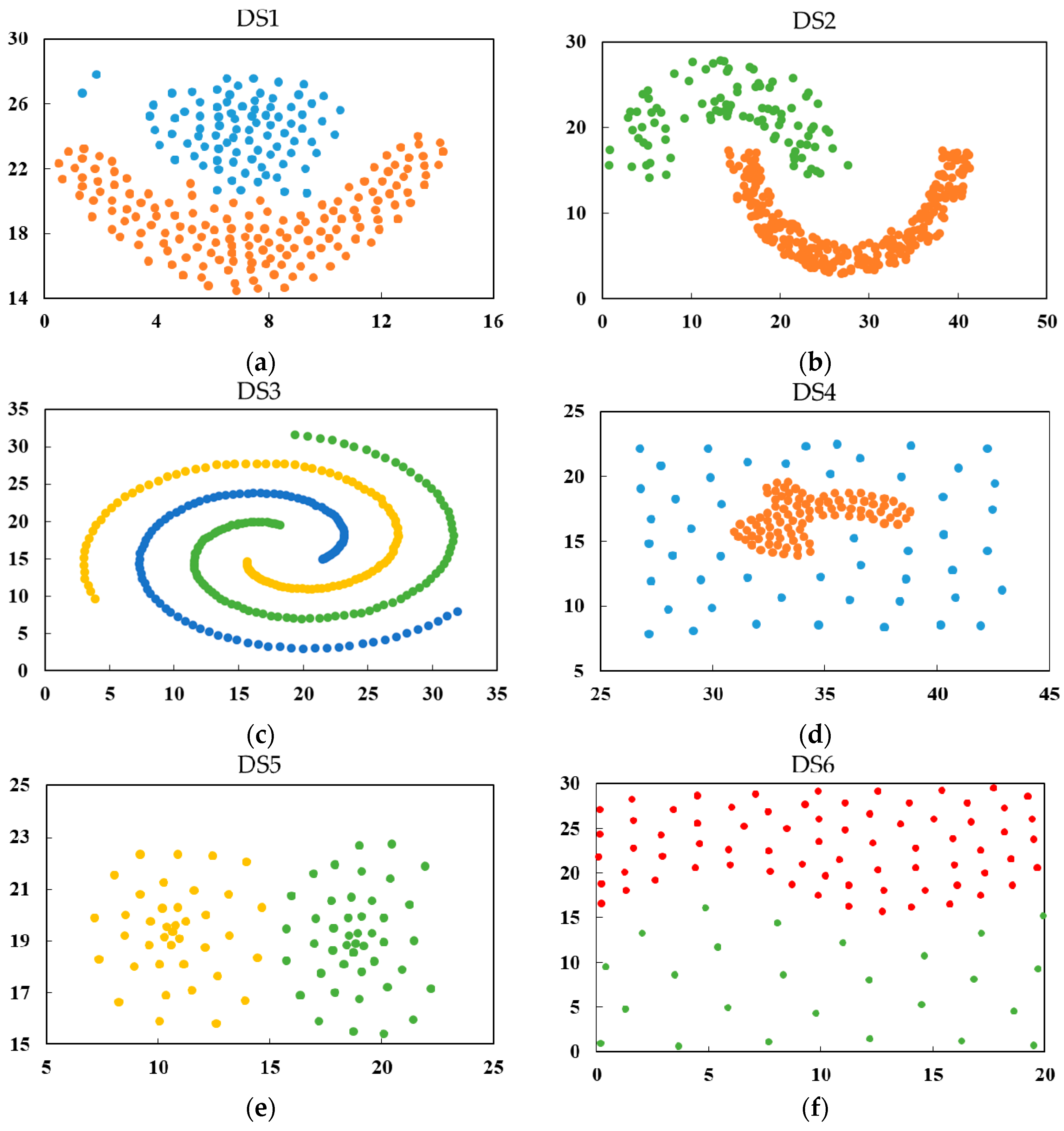
In this paper, the first three synthetic datasets, DS1, DS2 and DS3, are taken from the literature [26,27,28], while the next three DS4, DS5 and DS6 are from another previous study [17]. These datasets are illustrated in Figure 4 and Table 1, which are composed of clusters with diverse shapes and densities.
To demonstrate the superiority of SCMDOT when coping with different spatial datasets in this paper, SCDOT and DBSCAN are used for comparative analysis. With respect to the characteristics of spatial datasets, six synthetic datasets are separated into two groups. In Experiment 1, the first group including DS1–DS3 mostly focus on testing algorithms to examine whether they have the ability to detect clusters with arbitrary shapes. Some traditional partitioning methods and hierarchical algorithms, such as K-means and single-links, have difficulty in solving this problem. In comparison, three synthetic datasets, DS4–DS6, are used in Experiment 2 to show how seriously spatial objects with mixed densities can affect the accuracy of algorithms. This problem can be summarised in two situations. One is that the densities of different clusters are totally distinct, as shown in Figure 4d. The other one is that the density of cluster itself is unbalanced, as shown in Figure 4e. The two cases mentioned above are the main obstacles in some classical density-based clustering methods, such as DBSCAN and Ordering Points to Identify the Clustering Structure (OPTICS) [29], which makes them unable to set appropriate parameters to discover clusters with uneven density. Furthermore, the touching problems also include two types, which are taken into account in these datasets. One is the adjacent problem, in which sparse clusters are adjacent to compact clusters, as shown in Figure 4d,f. The other is the neck problem, as shown in Figure 4a,e.
The external clustering validity indices measure how close the clustering is to the predetermined benchmark classes. Therefore, the Adjust Rand Index (ARI) [30] and Adjusted Mutual Information (AMI) [31] are utilised to evaluate the quality of final clustering results in this section.
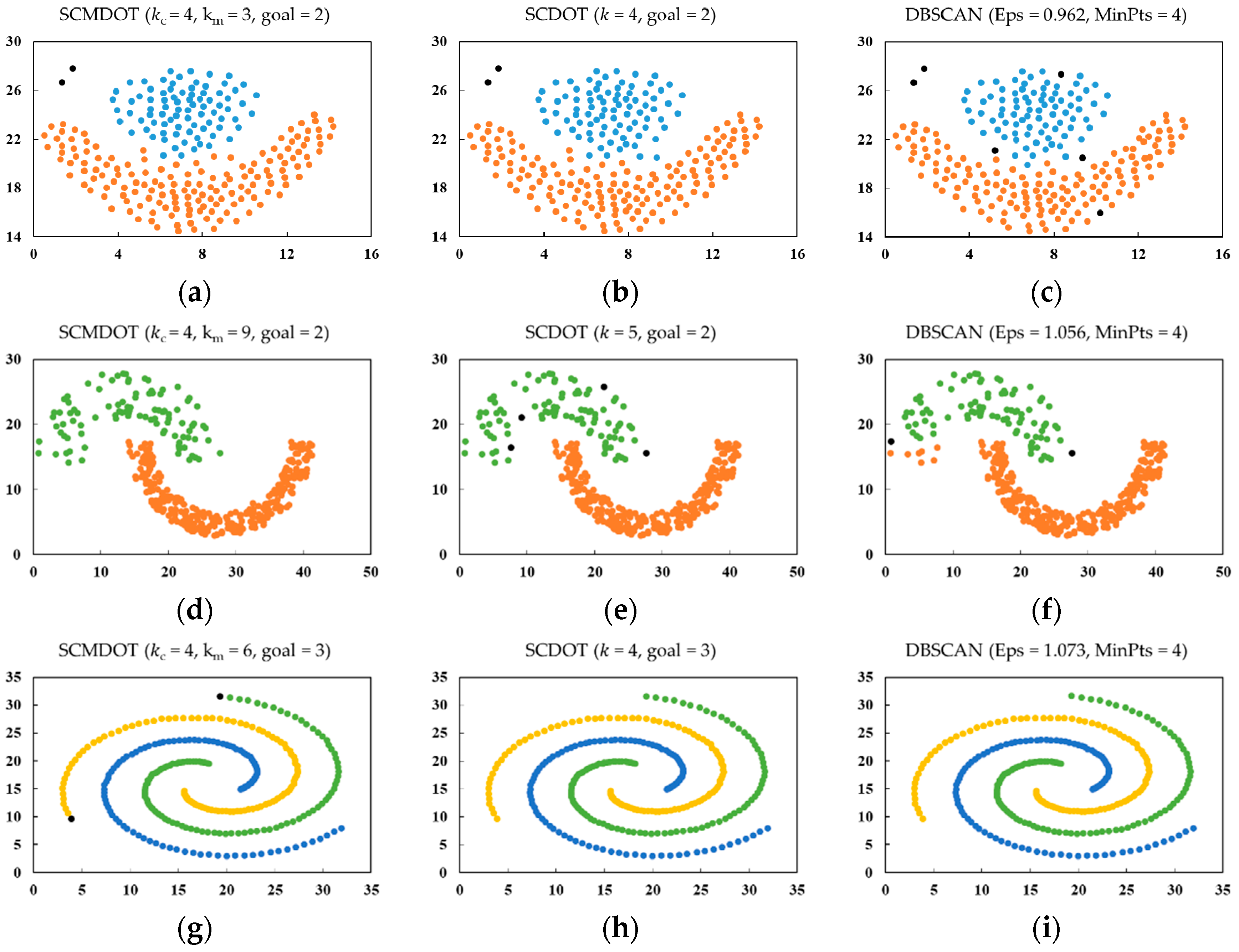
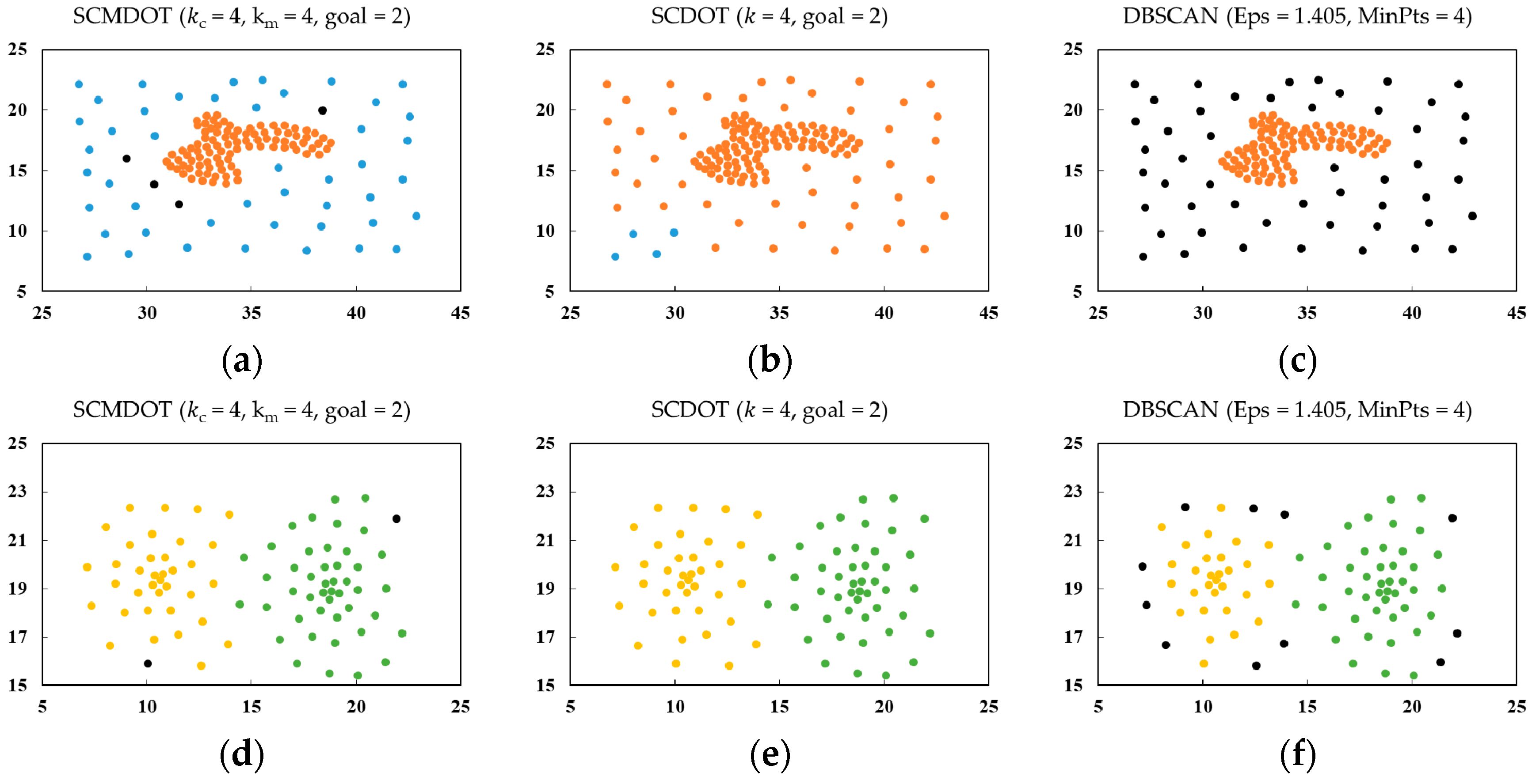
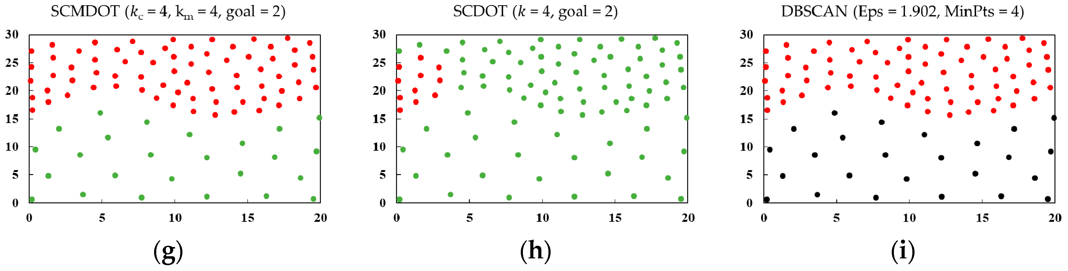
When comparing SCMDOT with SCDOT and DBSCAN, the setting of parameters was related to the original paper. For the SCDOT and DBSCAN algorithms, the parameters are respectively set as k = 4 (initial value) and MinPts = 4, which are based on the suggestions given in the methods. The clustering results are illustrated in Figure 5 and Figure 6.
The dataset DS1 is displayed in Figure 4a, which consists of a spherical cluster and a half ring-shaped cluster. Both clusters have similar densities, but they are adjacent to each other. Although all the algorithms can discover the expected clusters, it is difficult for DBSCAN to effectively handle the adjacent clusters.
The dataset DS2 is shown in Figure 4b. It contains two clusters that are shaped like crescents. These clusters are separate from each other and have relatively large differences in densities. Owning to the strategy in tackling inappropriate start points, SCMDOT has less noise when compared with others.
In Figure 4c, the dataset DS3 is composed of three spiral clusters, which are separated from each other at various distances. Additionally, each spiral cluster has an uneven density. All the three algorithms work well.
DS4, depicted in Figure 4d, consists of two clusters with extremely diverse densities and one of the clusters is surrounded by the other cluster. SCMDOT can easily distinguish the desired clusters because of its merging method. On the contrary, SCDOT and DBSCAN perform much worse under these conditions. For SCDOT algorithm, cutting off meaningless edges means that it is unable to find the genuine clusters. For DBSCAN, the variability in densities of two clusters results in a lack of tuning of suitable parameters.
DS5, as shown in Figure 4e, consists of two adjacent spherical clusters. The density of each cluster itself is uneven. SCMDOT and SCDOT perform well, but DBSCAN has lower accuracy since its clustering result contains too much noise.
The dataset DS6, displayed in Figure 4f, is composed of two wave-shaped clusters, which focuses on density rather than distance, which was labelled by Zahn as the density gradient. In contrast, SCMDOT has good performance with DS6, while SCDOT and DBSCAN perform badly. Furthermore, the problems encountered by the latter two methods are similar to DS4 above.
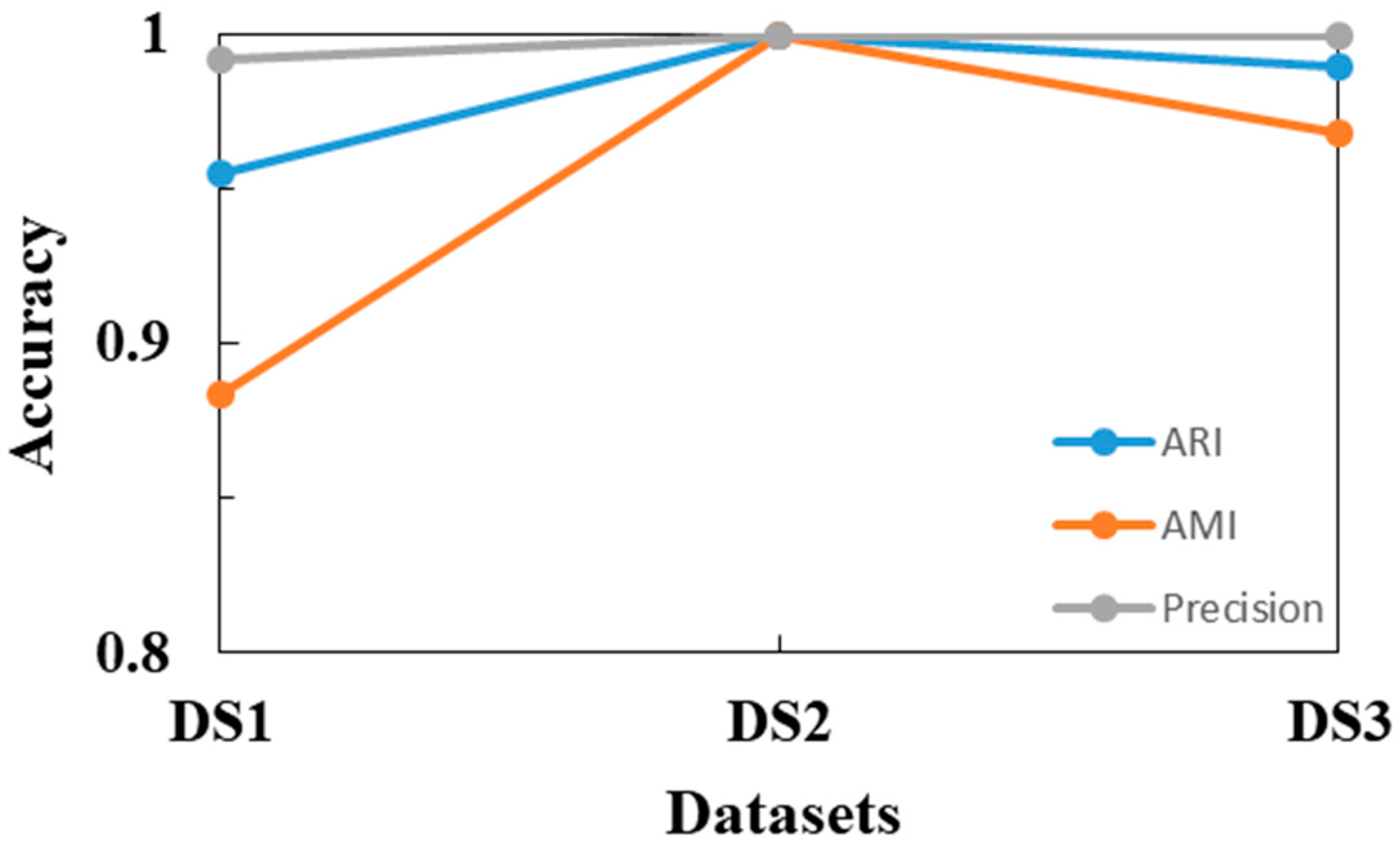
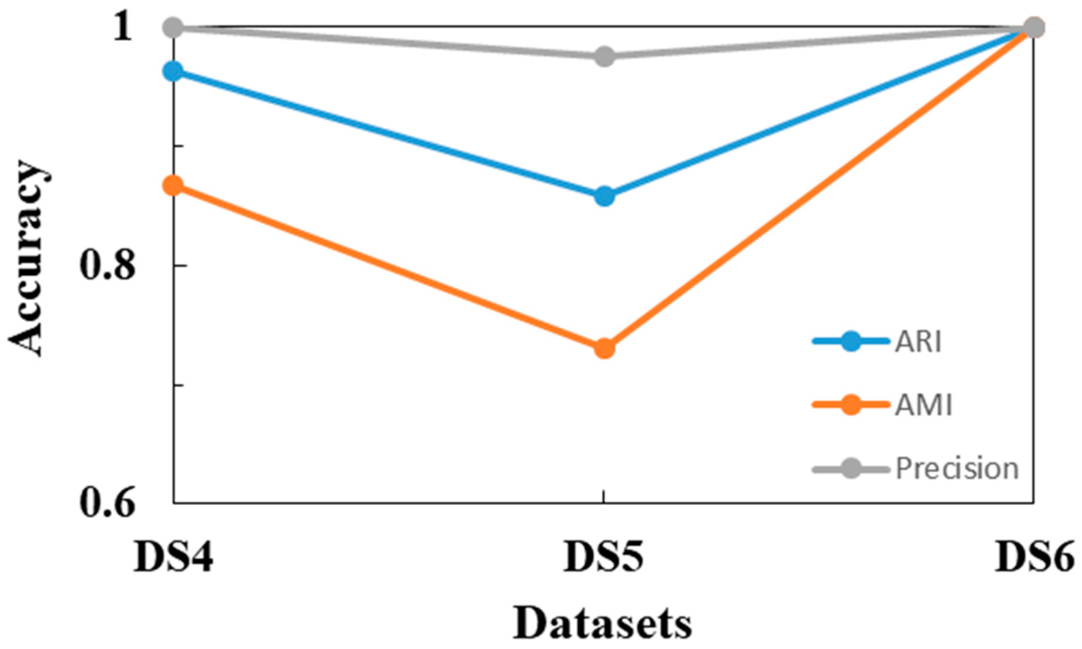
The corresponding Adjusted Rand index and Adjusted Mutual Information values of the clustering results on these six synthetic datasets are shown in Table 2 and Table 3. Furthermore, the accuracy results of SCMDOT are shown in Figure 7 and Figure 8, which indicates the superiority of our method in handling diverse spatial datasets.
4.2. Practical Applications of SCMDOT
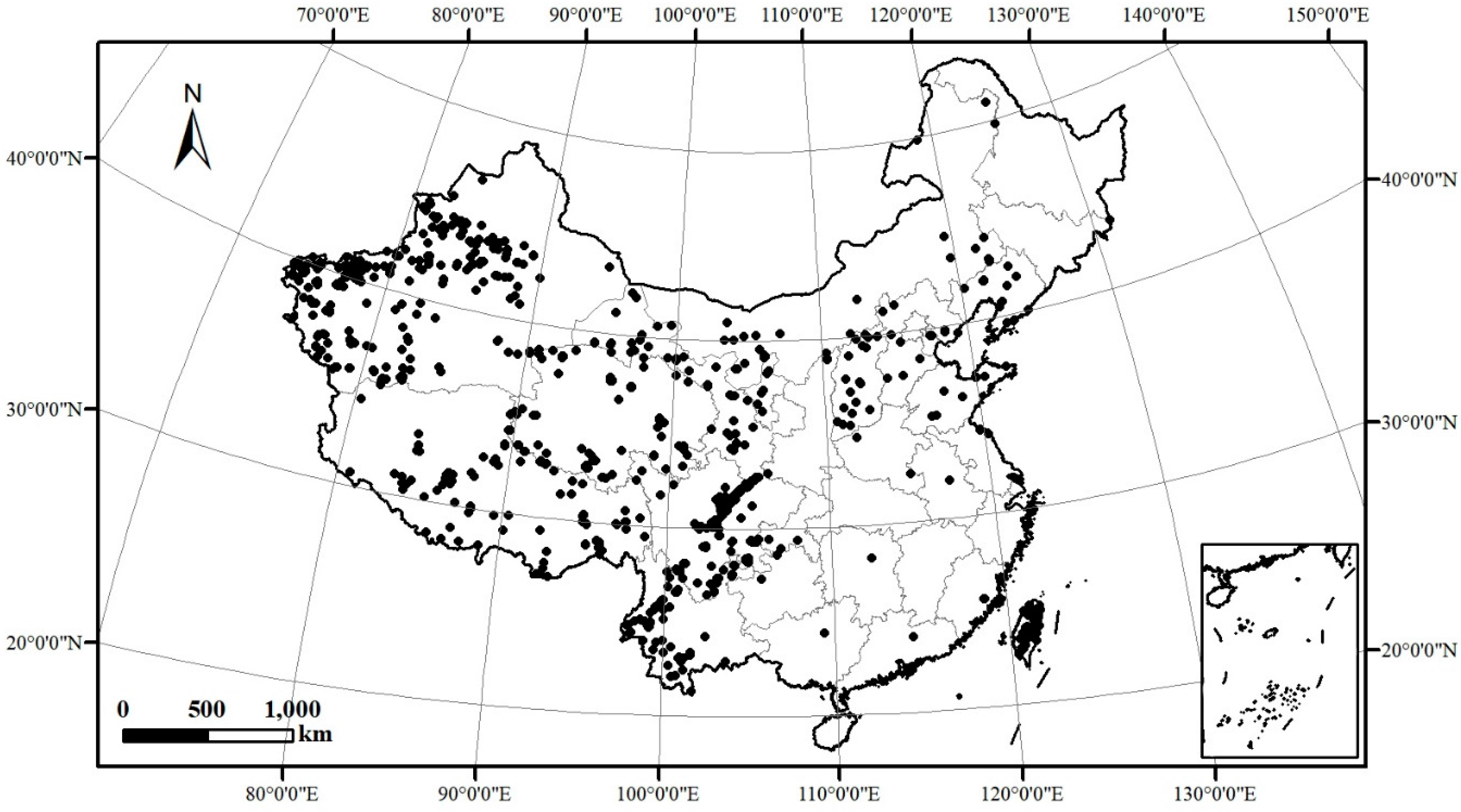
For the purpose of illustrating the practicability of the SCMDOT algorithm, the real-world application of earthquake clustering is utilised to discover the spatial distribution of active faults and find out the underlying cause of earthquakes. The geographical data of earthquakes in this paper are provided by the China Earthquake Data Centre (2009–2013; magnitude is greater than 3). The study area covers mainland China at the national level. There are 1349 locations of epicentres and information in the spatial database (the duplicate points are regarded as one point), which is shown in Figure 9.
Research shows that the phenomenon of earthquakes is usually generated by the movement of tectonic plates and has a close relevance to the trend of mountains, which indicates there is a strong spatial correlation for the clustering distribution of earthquakes. To better understand the spatial agglomeration patterns and characteristics of earthquakes in recent years, a multi-scale analysis of spatial clustering is applied.
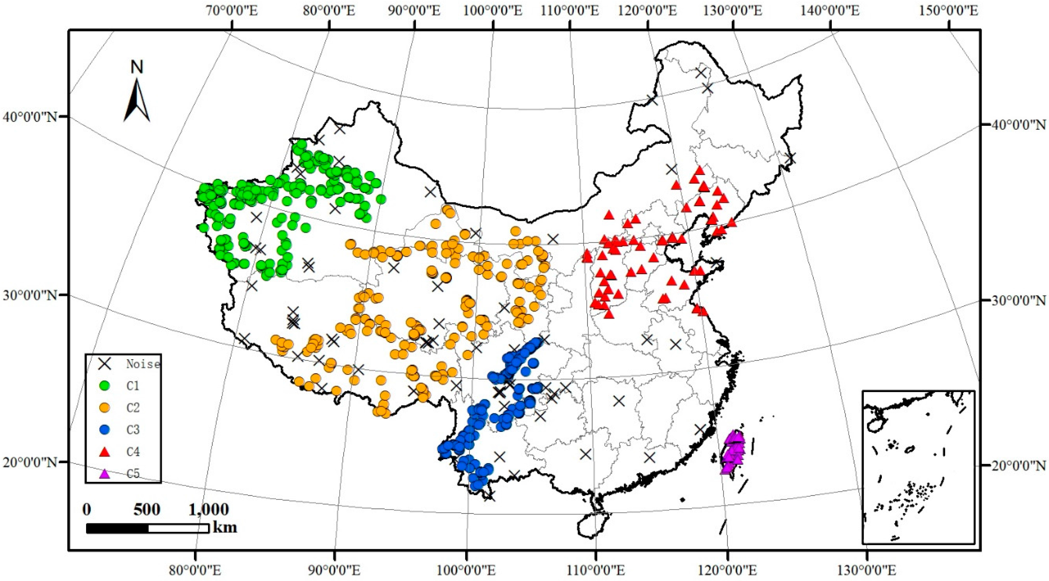
The clustering results of SCMDOT from macroscopic view is shown in Figure 10. It is obvious to see that there are five main seismic zones (C1–C5) in China, which are Xinjiang, Northwest, Southwest, North and Taiwan regions, respectively. Some isolated earthquakes are recognised as noise. Similar to Xinjiang and the Southwest seismic zone, most of Northwest China is located in the Qinghai–Tibet plateau, which is influenced by the collision between the India and Eurasia plates. As a result, this can set off devastating earthquakes. Furthermore, North and Taiwan seismic zones are located in the junction of the Asia–Europe and Pacific plate, which may result in the formation of seismically active faults.
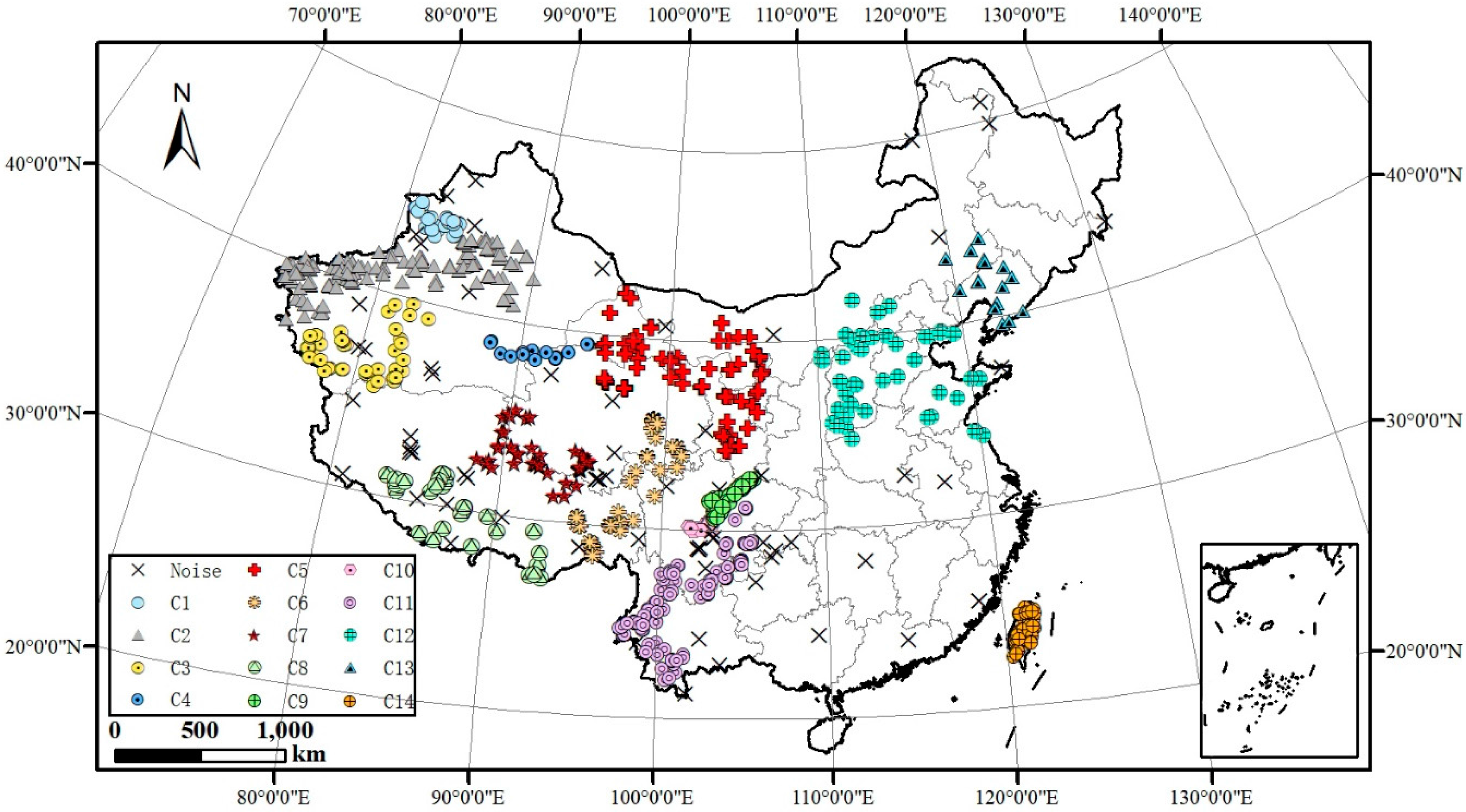
Moreover, by analysing earthquake clustering in a micro-perspective, more interesting relationships between clustering results and faults can be further investigated, as shown in Figure 11. The earthquake epicentres contained in relatively compact line-shaped clusters (C1–C4, C9–C11 and C14) mostly occur along the trend of seismically active mountains, such as the Tianshan Mountains, Qilian Mountains, Hengduan Mountains and Taiwan Mountains. The intense diastrophism of these big and main mountains may contribute to surrounding earthquakes. Furthermore, the rest of the clusters are relatively loose block-shaped clusters (C5–C8 and C12–C13). The cause of these clusters lies in many active faults in these regions and their directions differ from each other, which makes the distribution of earthquakes uneven and more complicated. According to the statistics of clusters, nearly half of the earthquakes occurred in the Sichuan–Yunnan region in the last five years. The obtained clustering results will be useful to provide reference for the research of the trends and movements of earthquake faults.
5. Discussion and Conclusions
In this paper, we introduce a novel clustering algorithm called SCMDOT, which is capable of dealing with the tricky cases of clusters with arbitrary shapes and uneven density. Inspired by the work of Cheng et al. [11], we provide a dynamic agglomerative model representing the original dataset through constructing MDOT. This is conducted with an innovative perspective in order to cover the shortages of coping with complex spatial structures. With the target of reinforcing spatial similarity for each cluster, we impose the additional constraints to rigorously restrain the growth of each DOT for ensuring that there is no dilemma in partitions, especially in some complicated situations. In addition, it is useful to effectively separate dense areas from regions of sparse areas. Considering the diversity of spatial patterns, our method adopts a heuristic strategy to be adaptive in selecting and exploring suitable parameters so as to meet different requirements of practical applications. Furthermore, cluster centres and noises can be easily identified based on MDOT. Essentially, cluster centres are regarded as the root nodes of sub-trees and noises are identified from inappropriate start points (explained in Section 3.3).
We conducted an extensive experimental study to evaluate our algorithm against SCDOT and DBSCAN on representative spatial datasets. Both synthetic and real-world experiments demonstrate that our proposed method is effective, more reliable and competitively robust with regards to varied cluster sizes, shapes and densities. However, the chaining problem is still a challenge for our method, which involves the noise or spatial object from one or more chains connecting two clusters. Our future work will focus on improving the robustness of SCMDOT in this area.
Acknowledgments
The research was supported by Key Science and Technology Plan Projects of Fujian Province (2015H0015), Education and Technology Plan Projects of Fujian Province (JAT160088), and Technology Innovation Foundation of Small and Medium-sized Enterprises of Fujian Province (2015C0042).
Author Contributions
Xiaozhu Wu and Hong Jiang conceived and designed the experiments; Hong Jiang performed the experiments; all the authors analysed the data; and Hong Jiang wrote the paper. All authors contributed with revising the manuscript.
Conflicts of Interest
The authors declare no conflict of interest.
References
- Yang, L.; Tian, F.; Smith, J.A.; Hu, H. Urban signatures in the spatial clustering of summer heavy rainfall events over the Beijing metropolitan region. J. Geophys. Res. Atmos. 2014, 119, 1203–1217. [Google Scholar] [CrossRef]
- Estivill-Castro, V.; Lee, I. Multi-level clustering and its visualization for exploratory spatial analysis. GeoInformatica 2002, 6, 123–152. [Google Scholar] [CrossRef]
- Sluydts, V.; Heng, S.; Coosemans, M.; Roey, K.V.; Gryseels, C.; Canier, L.; Kim, S.; Khim, N.; Siv, S.; Mean, V. Spatial clustering and risk factors of malaria infections in ratanakiri province, cambodia. Malar. J. 2014, 13, 387. [Google Scholar] [CrossRef] [PubMed]
- Jagla, E.A.; Kolton, A.B. A mechanism for spatial and temporal earthquake clustering. J. Geophys. Res. Atmos. 2010, 115, 100–104. [Google Scholar] [CrossRef]
- Deng, M.; Liu, Q.; Cheng, T.; Shi, Y. An adaptive spatial clustering algorithm based on delaunay triangulation. Comput. Environ. Urban Syst. 2011, 35, 320–332. [Google Scholar] [CrossRef]
- Jain, A.K.; Murty, M.N.; Flynn, P.J. Data clustering: A review. ACM Comput. Surv. 1999, 31, 264–323. [Google Scholar] [CrossRef]
- Xu, R.; Wunsch, D. Survey of clustering algorithms. IEEE Trans. Neural Netw. 2005, 16, 645–678. [Google Scholar] [CrossRef] [PubMed]
- MacQueen, J. Some Methods for Classification and Analysis of Multivariate Observations. In Proceedings of the Fifth Berkeley Symposium on Mathematical Statistics and Probability, Berkeley, CA, USA, 21 June–18 July 1965 and 27 December 1965–7 January 1966; pp. 281–297. [Google Scholar]
- Ester, M.; Kriegel, H.-P.; Sander, J.; Xu, X. A density-based algorithm for discovering clusters in large spatial databases with noise. In Proceedings of the Second International Conference on Knowledge Discovery and Data Mining (KDD-96), Portland, OR, USA, 2–4 August 1996; pp. 226–231. [Google Scholar]
- Frey, B.J.; Dueck, D. Clustering by passing messages between data points. Science 2007, 315, 972. [Google Scholar] [CrossRef] [PubMed]
- Cheng, Q.; Lu, X.; Liu, Z.; Huang, J.; Cheng, G. Spatial clustering with density-ordered tree. Phys. A Stat. Mech. Appl. 2016, 460, 188–200. [Google Scholar] [CrossRef]
- Rodriguez, A.; Laio, A. Clustering by fast search and find of density peaks. Science 2014, 344, 1492–1496. [Google Scholar] [CrossRef] [PubMed]
- Mehmood, R.; Zhang, G.; Bie, R.; Dawood, H.; Ahmad, H. Clustering by fast search and find of density peaks via heat diffusion. Neurocomputing 2016, 208, 210–217. [Google Scholar] [CrossRef]
- Xu, J.; Wang, G.; Deng, W. DenPEHC: Density peak based efficient hierarchical clustering. Inf. Sci. 2016, 373, 200–218. [Google Scholar] [CrossRef]
- Schaeffer, S.E. Graph clustering. Comput. Sci. Rev. 2007, 1, 27–64. [Google Scholar] [CrossRef]
- Karypis, G.; Han, E.H.; Kumar, V. Chameleon: A hierarchical clustering algorithm using dynamic modeling. Computer 1999, 32, 68–75. [Google Scholar] [CrossRef]
- Zahn, C.T. Graph-theoretical methods for detecting and describing gestalt clusters. IEEE Trans. Comput. 1971, C-20, 68–86. [Google Scholar] [CrossRef]
- Zhong, C.; Miao, D.; Wang, R. A graph-theoretical clustering method based on two rounds of minimum spanning trees. Pattern Recognit. 2010, 43, 752–766. [Google Scholar] [CrossRef]
- Zhong, C.; Miao, D.; Nti, P. Minimum spanning tree based split-and-merge: A hierarchical clustering method. Inf. Sci. 2011, 181, 3397–3410. [Google Scholar] [CrossRef]
- Guo, D.; Wang, H. Automatic region building for spatial analysis. Trans. GIS 2011, 15, 29–45. [Google Scholar] [CrossRef]
- Guha, S.; Rastogi, R.; Shim, K. CURE: An Efficient Clustering Algorithm for large Databases. In Proceedings of the ACM-SIGMOD International Conference on Management of Data, Seattle, WA, USA, 1–4 June 1998; pp. 73–84. [Google Scholar]
- Guha, S.; Rastogi, R.; Shim, K. ROCK: A robust clustering algorithm for categorical attributes. Inf. Syst. 2000, 25, 345–366. [Google Scholar] [CrossRef]
- Lee, J.S.; Olafsson, S. A meta-learning approach for determining the number of clusters with consideration of nearest neighbors. Inf. Sci. 2013, 232, 208–224. [Google Scholar] [CrossRef]
- Lee, J.-S.; Olafsson, S. Data clustering by minimizing disconnectivity. Inf. Sci. 2011, 181, 732–746. [Google Scholar] [CrossRef]
- Bentley, J.L. Multidimensional binary search trees used for associative searching. Commun. ACM 1975, 18, 509–517. [Google Scholar] [CrossRef]
- Fu, L.; Medico, E. Flame, a novel fuzzy clustering method for the analysis of DNA microarray data. BMC Bioinform. 2007, 8, 3. [Google Scholar] [CrossRef] [PubMed]
- Jain, A.K.; Law, M.H.C. Data clustering: A user′s dilemma. In Proceedings of the Pattern Recognition and Machine Intelligence, First International Conference, Kolkata, India, 20–22 December 2005; pp. 1–10. [Google Scholar]
- Chang, H.; Yeung, D.Y. Robust path-based spectral clustering. Pattern Recognit. 2008, 41, 191–203. [Google Scholar] [CrossRef]
- Ankerst, M.; Breunig, M.M.; Kriegel, H.-P.; Sander, J. OPTICS: Ordering points to identify the clustering structure. In Proceedings of the ACM-SIGMOD International Conference on Management of Data, Philadelphia, PA, USA, 31 May–3 June 1999; pp. 49–60. [Google Scholar]
- Rand, W.M. Objective criteria for the evaluation of clustering methods. J. Am. Stat. Assoc. 1971, 66, 846–850. [Google Scholar] [CrossRef]
- Vinh, N.X.; Epps, J.; Bailey, J. Information theoretic measures for clusterings comparison: Variants, properties, normalization and correction for chance. J. Mach. Learn. Res. 2010, 11, 2837–2854. [Google Scholar]
Figure 1.
Examples of representative spatial patterns. (a–f) Spatial patterns include clusters with different shapes, sizes and densities.
Figure 1.
Examples of representative spatial patterns. (a–f) Spatial patterns include clusters with different shapes, sizes and densities.

Figure 2.
The process of Spatial Clustering with Multiple Density-Ordered Trees (SCMDOT) consists of three main stages including the pruning stage, the constructing stage and the merging stage. (a) Original dataset; (b) Prune inappropriate start point; (c) Construct Multiple Density-Ordered Trees (MDOT); (d) Merge MDOT into final clusters; (e) Identify and exclude noise; (f) Final clusters.

Figure 3.
Illustration of the stage of constructing Multiple Density-Ordered Trees (MDOT): (a) Original dataset; (b) Example of the growth of MDOT; and (c) Result of constructing MDOT.
Figure 3.
Illustration of the stage of constructing Multiple Density-Ordered Trees (MDOT): (a) Original dataset; (b) Example of the growth of MDOT; and (c) Result of constructing MDOT.

Figure 4.
Illustration of the six original synthetic datasets. (a) Experimental data of DS1; (b) Experimental data of DS2; (c) Experimental data of DS3; (d) Experimental data of DS4; (e) Experimental data of DS5; (f) Experimental data of DS6.
Figure 4.
Illustration of the six original synthetic datasets. (a) Experimental data of DS1; (b) Experimental data of DS2; (c) Experimental data of DS3; (d) Experimental data of DS4; (e) Experimental data of DS5; (f) Experimental data of DS6.

Figure 5.
Illustration of clustering results in Experiment 1. (a–c) The clustering results of DS1; (d–f) The clustering results of DS2; (g–i) The clustering results of DS3.
Figure 5.
Illustration of clustering results in Experiment 1. (a–c) The clustering results of DS1; (d–f) The clustering results of DS2; (g–i) The clustering results of DS3.

Figure 6.
Illustration of clustering results in Experiment 2. (a–c) The clustering results of DS4; (d–f) The clustering results of DS5; (g–i) The clustering results of DS6.
Figure 6.
Illustration of clustering results in Experiment 2. (a–c) The clustering results of DS4; (d–f) The clustering results of DS5; (g–i) The clustering results of DS6.


Figure 7.
The accuracy values of SCMDOT in Experiment 1.

Figure 8.
The accuracy values of SCMDOT in Experiment 2.

Figure 9.
Locations of the earthquakes in China (2009–2013 with a magnitude greater than 3).

Figure 10.
Clustering results for the earthquake database using the SCMDOT algorithm from the macroscopic view.
Figure 10.
Clustering results for the earthquake database using the SCMDOT algorithm from the macroscopic view.

Figure 11.
Clustering results for the earthquake database by SCMDOT algorithm in a micro-perspective.
Figure 11.
Clustering results for the earthquake database by SCMDOT algorithm in a micro-perspective.


Table 1.
Detailed description of datasets.
| Data Set | Data Size (N) | Dimensionality (d) | Number of Clusters (K) |
|---|---|---|---|
| DS1 | 240 | 2 | 2 |
| DS2 | 373 | 2 | 2 |
| DS3 | 312 | 2 | 3 |
| DS4 | 142 | 2 | 2 |
| DS5 | 83 | 2 | 2 |
| DS6 | 97 | 2 | 2 |
Table 2.
Results in Adjust Rand index (ARI) and Adjusted Mutual Information (AMI) for DS1, DS2, and DS3 datasets.
Table 2.
Results in Adjust Rand index (ARI) and Adjusted Mutual Information (AMI) for DS1, DS2, and DS3 datasets.
| SCMDOT | SCDOT | DBSCAN | |||||||
|---|---|---|---|---|---|---|---|---|---|
| ARI | AMI | Noise Number | ARI | AMI | Noise Number | ARI | AMI | Noise Number | |
| DS1 | 0.955 | 0.884 | 2 | 0.988 | 0.942 | 2 | 0.939 | 0.817 | 6 |
| DS2 | 1 | 1 | 0 | 0.989 | 0.927 | 4 | 0.976 | 0.859 | 2 |
| DS3 | 0.990 | 0.968 | 2 | 1 | 1 | 0 | 1 | 1 | 0 |
Table 3.
Results in Adjust Rand index (ARI) and Adjusted Mutual Information (AMI) for DS4, DS5, and DS6 datasets.
Table 3.
Results in Adjust Rand index (ARI) and Adjusted Mutual Information (AMI) for DS4, DS5, and DS6 datasets.
| SCMDOT | SCDOT | DBSCAN | |||||||
|---|---|---|---|---|---|---|---|---|---|
| ARI | AMI | Noise Number | ARI | AMI | Noise Number | ARI | AMI | Noise Number | |
| DS4 | 0.963 | 0.867 | 4 | 0.049 | 0.040 | 0 | 0 | 0 | 50 |
| DS5 | 0.859 | 0.730 | 2 | 0.905 | 0.855 | 0 | 0.729 | 0.563 | 11 |
| DS6 | 1 | 1 | 0 | −0.090 | 0.054 | 0 | 0 | 0 | 25 |
© 2017 by the authors. Licensee MDPI, Basel, Switzerland. This article is an open access article distributed under the terms and conditions of the Creative Commons Attribution (CC BY) license (http://creativecommons.org/licenses/by/4.0/).
Share and Cite
MDPI and ACS Style
Wu, X.; Jiang, H.; Chen, C. SCMDOT: Spatial Clustering with Multiple Density-Ordered Trees. ISPRS Int. J. Geo-Inf. 2017, 6, 217. https://0-doi-org.brum.beds.ac.uk/10.3390/ijgi6070217
AMA Style
Wu X, Jiang H, Chen C. SCMDOT: Spatial Clustering with Multiple Density-Ordered Trees. ISPRS International Journal of Geo-Information. 2017; 6(7):217. https://0-doi-org.brum.beds.ac.uk/10.3390/ijgi6070217
Chicago/Turabian StyleWu, Xiaozhu, Hong Jiang, and Chongcheng Chen. 2017. "SCMDOT: Spatial Clustering with Multiple Density-Ordered Trees" ISPRS International Journal of Geo-Information 6, no. 7: 217. https://0-doi-org.brum.beds.ac.uk/10.3390/ijgi6070217
Note that from the first issue of 2016, this journal uses article numbers instead of page numbers. See further details here.