Comparative Analysis on Topological Structures of Urban Street Networks


Department of Urban Planning and Environment, Royal Institute of Technology, Drottning Kristinas väg 30, 100 44 Stockholm, Sweden
*
Author to whom correspondence should be addressed.
ISPRS Int. J. Geo-Inf. 2017, 6(10), 295; https://0-doi-org.brum.beds.ac.uk/10.3390/ijgi6100295
Submission received: 3 July 2017
/
Revised: 17 September 2017
/
Accepted: 19 September 2017
/
Published: 24 September 2017
Abstract
:Street systems are the backbone of cities. With global urbanization and economic development, street systems have undergone significant development along with the growth of cities. In this paper, the authors select three cities with varying sizes, histories, locations, and growth dynamics: Stockholm, Toronto, and Nanjing. We analyze topological structures of their public street systems based on GIS and complex network theory. Considering the planarity of street systems, we first calculate various topological measures, including α, β, and γ indices, and density. This is followed by comparing three centrality measures, i.e., degree, betweenness, and closeness in complex network theory. In this part, we investigate these characteristics of nodes and edges in a primal representation, and discuss their relations with urban growth mechanisms.
1. Introduction
Street networks are the backbone of cities and correlate with urban development. In the real world, different cities show distinct street patterns due to various historical reasons, geographic surroundings, socio-cultural environments, economic conditions, and more. In this sense, exploring street patterns can reveal many underlying features of a city; therefore, it is of the utmost importance for city planners and policy-makers.
As a typical class of planar systems, much attention has been paid to urban street systems from different perspectives. In the 1960s, quantitative geographers and transport researchers defined and calculated the planarity of transport systems [1,2]. Afterward, many global measures of heterogeneity, connectivity, accessibility, and interconnectivity were proposed to explore the topological structure of spatial systems [3,4,5,6]. In contrast, space syntax analyzes spatial configurations on the basis of the spatial and social relationship in urban street systems; therefore, it provides a good way to sketch street networks and urban morphology from a topological perspective [7,8]. On the other hand, traffic flows and travel patterns of citizens also invoke the interest of researchers considering the importance of street systems in shaping people’s daily lives [9,10].
Since proposing the complex network theory late last century, transport systems, as a typical instance of spatial networks, have made progress from various subjects [11,12,13,14,15,16]. Topological properties and structures have gained the most attention [11,14,17,18,19]. Different representations and statistical measures are widely discussed as the first step to study transport systems [16,20,21]. As a traditional measure in complex network analysis, centrality was introduced to explore transport systems, including aviation systems [22], street networks [14], metro systems [23], and bus stop systems [24,25,26]. Many studies emerged in this field, and some common features, such as the small-world effect and the power-law distribution are found across transportation systems of different sizes [27,28,29,30,31]. In comparison, empirical analyses are constrained into topological features, and limited focus was put on spatial structures from a complex network perspective [28,32,33]. Street networks are more constrained by geographic factors compared to aviation systems and public transport systems. Some effort is made to extend complex network properties to reveal the planarity of real street systems [34]. For example, the cell degree is proposed to measure the number of first neighbors of a cell in a street system based on the node degree, which is a traditional measure in complex network analyses [13]. However, street networks are a complicated outcome of city evolution, which would in turn shape the future urban development pattern. Although complex network measures can depict many underlying features and mechanisms of street systems, to the authors’ knowledge, their relation to urban patterns are still unclear and require additional study.
The primal aim of this paper is to discuss the street patterns from both the spatial and the topological perspectives and compare them within different urban-pattern frameworks. To this end, we selected three different cities as study cases (i.e., Stockholm, Sweden; Nanjing, China; and Toronto, Canada). They are located on different continents and possess distinct geographic backgrounds, as well as urban development patterns, which are supposed to have a very large effect on their transportation networks.
The remainder of the paper takes the following form: Section 2 introduces the study area and data preprocessing. Moreover, the research methods adopted in this paper are also investigated in this section. Section 3 describes the planarity of three networks in terms of their different urban patterns. Section 4 discusses and compares the different topological network measures of three cities. The conclusion summarizes our findings and indicates future directions.
2. Data and Methods
2.1. Data Collection
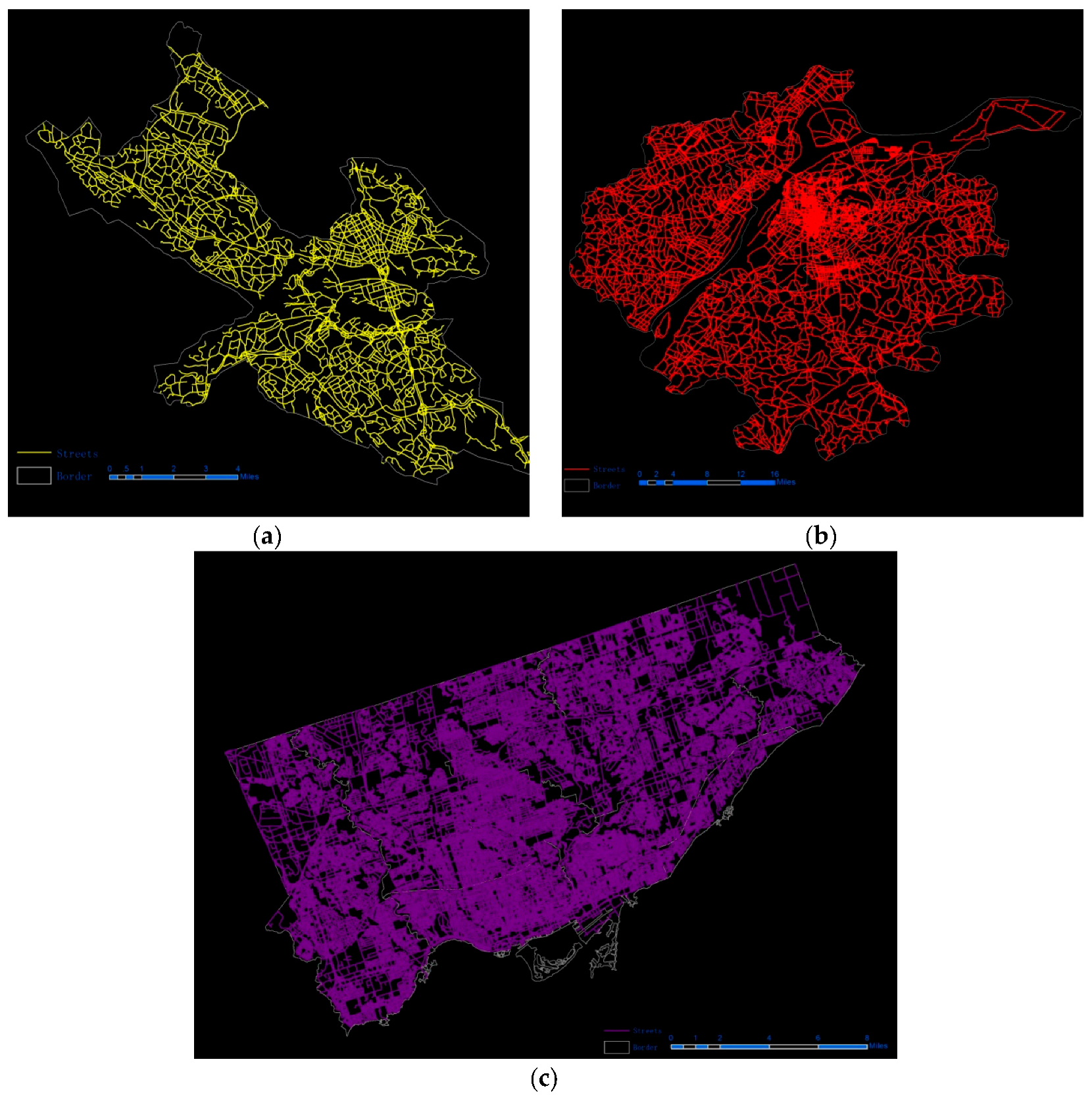
In this paper, three cities will be discussed: Stockholm, Sweden; Nanjing, China; and Toronto, Canada. They present distinct properties in terms of urban population, area and economic development (Table 1). Stockholm is the capital as well as the most populous city of Sweden and on the Scandinavian Peninsula (Figure 1a). Compared to Nanjing and Toronto, Stockholm possesses the smallest numbers in GDP, area, and population; however, it has been undergoing a rapid development over this past decade. Yet, it has the highest mean income for its inhabitants. Nanjing is the provincial capital of the Jiangsu Province of China, and the eighth largest city in China (Figure 1b). Considering the changes in the administrative divisions in 2012, we included the main central districts (which consists of four districts: Qinghuai, Gulou, Jianye, and Xuanwu), Pukou district, Jiangning district, and Qixia district in this study. With the rapid urbanization and economic development in China, Nanjing has grown and extended, in urban area and population, at a fast pace since 2000. Toronto is the capital of the Province of Ontario and the most populous city in Canada. It has experienced a surge in both economics and population for many years (Figure 1c). The GDP of the city of Toronto reached $143.8 billion in 2012. It is worth mentioning that Toronto is also known for its strict urban planning. In this sense, it can be seen as a planned city, whereas Stockholm and Nanjing are more self-organized in terms of their spatial patterns. Note that every city might be affected by natural or artificial constraints, more or less. For example, Stockholm is located by the ocean, Toronto is constrained on one side by a lake, and administrative zoning imposes a complicated effect on Nanjing’s street network. In this sense, geographic constraints can be ignored in this comparative analysis.
The data used in this work consists of two parts, the statistical data and the map data. The statistical data of Stockholm comes from the Statistics Bureau of Sweden website [35]. The statistical data of Nanjing was extracted from the Nanjing Statistical Yearbook 2013. It is worth noting that in consideration of the different statistical scales in China, we selected the urban area to compare Nanjing with the other cities. The statistical data of Toronto is extracted from the Statistics Canada website [36] and the Map and Data Library of the University of Toronto [37]. On the other hand, the map data are processed in ArcGIS 10.1 ESRI (Redlands, CA, USA) by the authors themselves.
2.2. Network Representation
A graph G consists of the set of vertices (nodes) V and the set of edges (links) E [38]. There are two different representation methods for urban street networks (i.e., the primal approach and the dual approach). The primal representation is a natural and intuitional approach, which takes just the road segments as links, and intersections or the ends of roads as nodes for an urban street network [21]. This method is similar to social networks or airport networks [16]. In this study, we select this method to represent three street systems to provide a more objective picture. In contrast, the dual representation could introduce more subjectivity. For this method, street segments are taken as nodes, and if two segments intersect, an edge between them will be constructed [39]. In this sense, defining the segments (i.e., the meaning of the nodes), becomes the problem. This topic has been widely discussed by researchers from various perspectives [14,20]; however, we do not give detailed explanations here due to space limitations.
2.3. Planarity
In graph theory, a planar graph indicates a graph in which all edges intersect only at their endpoints. To avoid unnecessary topological complication, we assume that the vertices of a graph are the street intersections in a city and the extremes of the dead-end roads, while the edges are the street fragments connecting the intersections. All freeways, tunnels, or overbridges are mapped to the surface transportation network, and only one segment is kept if a duplicate is detected. In this sense, a street system can be regarded as a typical planar network.
The alpha coefficient α is also called the meshedness coefficient, which is used to measure the structure of cycles in a planar systems. It can be written as [3]:
Here, NE and NV represent the number of edges E and nodes N in a planar network. According to the Euler’s formula, the number of cells in a planar network can be calculated as NE − NV + 1, and the maximum number of cells in a network equals 2NV − 5. In this case, the alpha coefficient can be seen as the ratio of the real number of cells and the maximum number of cells in a network. Therefore. the value of the alpha coefficient should lie in the range between 0 and 1.
The beta coefficient β is very straightforward. It can be written as the ratio of the number of edges and the number of nodes in a network. It measures the connectivity of a network, and a larger value indicates a better connectivity:
The gamma index γ is a measure of the relation between the real number of edges and the number of all possible edges in a network, which can be calculated as:
Likewise, NE is the number of edges and NV indicates the number of nodes in a network. 3(NV − 2) calculates the maximum edges for a planar network which is composed of NV nodes. Therefore, the value of the gamma index is between 0 and 1, and 1 means a fully-connected graph.
Characteristic path length Lgeo reflects the internal structure of a network by containing the internal separations of all nodes, and is defined as:
where NV represents the numbers of nodes, while dij indicates the minimum length of the paths that connect two arbitrary vertices, i.e., the graph geodesic distance between the two vertices in a planar network.
2.4. Node Measures
2.4.1. Degree Centrality
For node i, its degree centrality measures the number of edges connected to it, which can be written as [40]:
In which i, j are nodes in the network V, and aij is the entry value in the adjacency matrix, which equals 1 when i and j are connected and 0 when they are not. Note that in this study, we do not include the case of i = j, which indicates a loop in the network.
2.4.2. Betweenness Centrality
The betweenness centrality reflects the level of intermediate importance. It is measured by the probability that a node i is passed by the shortest paths between all node pairs in the network [40,41,42], that is:
Here njh(i) is the number of shortest paths between node j and h which pass the vertex i, and njh is the total number of shortest paths between them. NV indicates the number of nodes in the network.
2.4.3. Closeness Centrality
The closeness centrality calculates the distance from a node i to all other nodes in a system, which can be written as:
Here, dij represents the shortest path length between node i and j, and NV is the number of nodes in the network. In our study, dij represents the geodesic distance that measures the accessibility from a planar perspective instead of the spatial road distance.
2.4.4. Clustering Coefficient
The clustering coefficient is calculated as the probability that two neighbors of a node are likely to be connected themselves, which can be used to quantify the degree of clustering of a graph. Accordingly, the clustering coefficient for the entire network is:
Here, mi indicates the number of edges between the first neighbors of node i, and represents degree centrality of node i in the network.
3. Planarity of the Urban Street Networks in the Primal Representation
3.1. α, β, and γ Coefficients and Network Density
In this part, we calculated some basic coefficients of the three systems, including the α, β, and γ coefficients, the network density, and more. As discussed in the last section, these coefficients can depict different features of the cellular structure of planar systems.
In Table 2, Toronto possesses the largest network size in terms of the number of both nodes and edges, which is almost four times that of Nanjing and ten times that of Stockholm. In comparison, Stockholm presents the smallest network with the smallest values in all coefficients. It is worth noting that Nanjing gives the biggest values in Ltotal, cc, α, β, and γ coefficients; however, it does not agree with the conclusion based on the empirical analysis of metropolitan areas in the United States [6], which indicates that the values of coefficients increase with the size of the city. It is worth noting that the meshedness coefficients of the three systems are small because of the lack of triangles in real cities. This conclusion coincides with the findings of Bual et al. [34] and Crucitti et al. [43]. On the other hand, some significant differences are detected between self-organized and planned cities. For example, although the numbers of nodes and links in Toronto are much greater than those of Nanjing, the total street length of the former is less than the latter. Additionally, the clustering coefficient of the system of Nanjing is also larger than that of Toronto. This means that, for an organized street system, the first neighbors of a node are more inclined to connect with each other, which also conforms to the scenario in the real world.
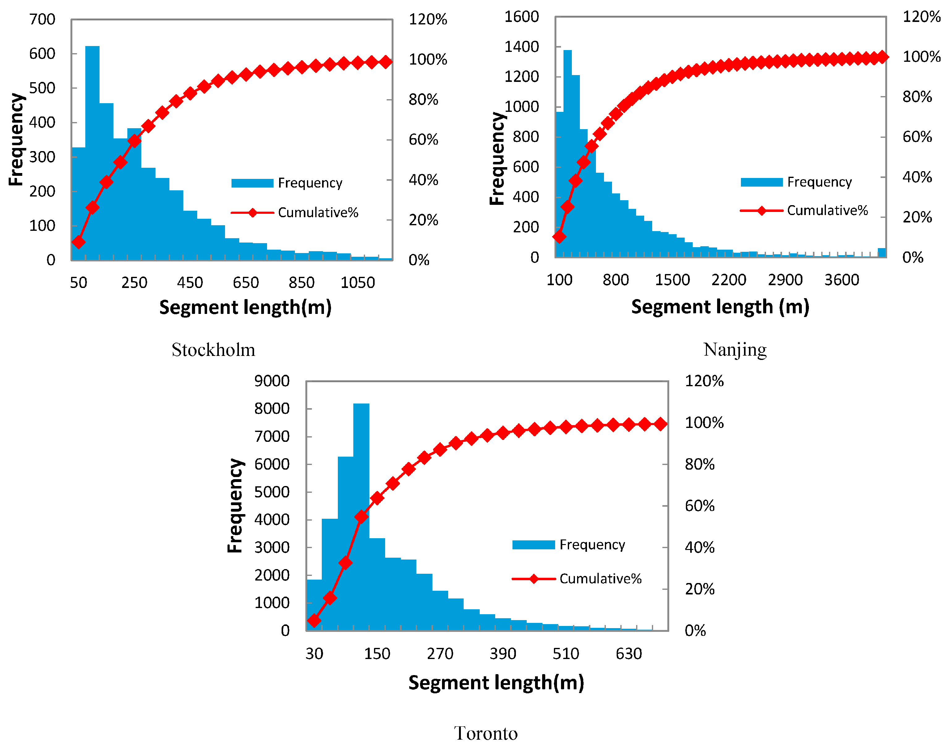
3.2. Length Distribution
All three systems show a clear bias toward shorter segments, which is unsurprising because short segments are more efficient for street systems. However, when we look closely, the systems show some striking differences. In Figure 2, we present the histograms of street lengths in meters in the urban street systems of Stockholm, Nanjing, and Toronto. Our findings here conflict with the conclusion that self-organized cities present a single peak distribution, which the planned cities did not [44]; however, there are some differences between self-organized and strictly-planned systems. Common to the city of Stockholm and Nanjing is a relatively even distribution of segment lengths. As a result, 86% of the streets are shorter than 500 m, while 2% are longer than 1000 m for the city of Stockholm. For the city of Nanjing, only 55% of the street segments are shorter than 500 m. In contrast, 20% of the segments are longer than 1000 m, of which 25% are longer than 2000 m. As a strictly planned city, Toronto possesses street segments and 98% are shorter than 500 m, while only 0.1% are longer than 1000 m.
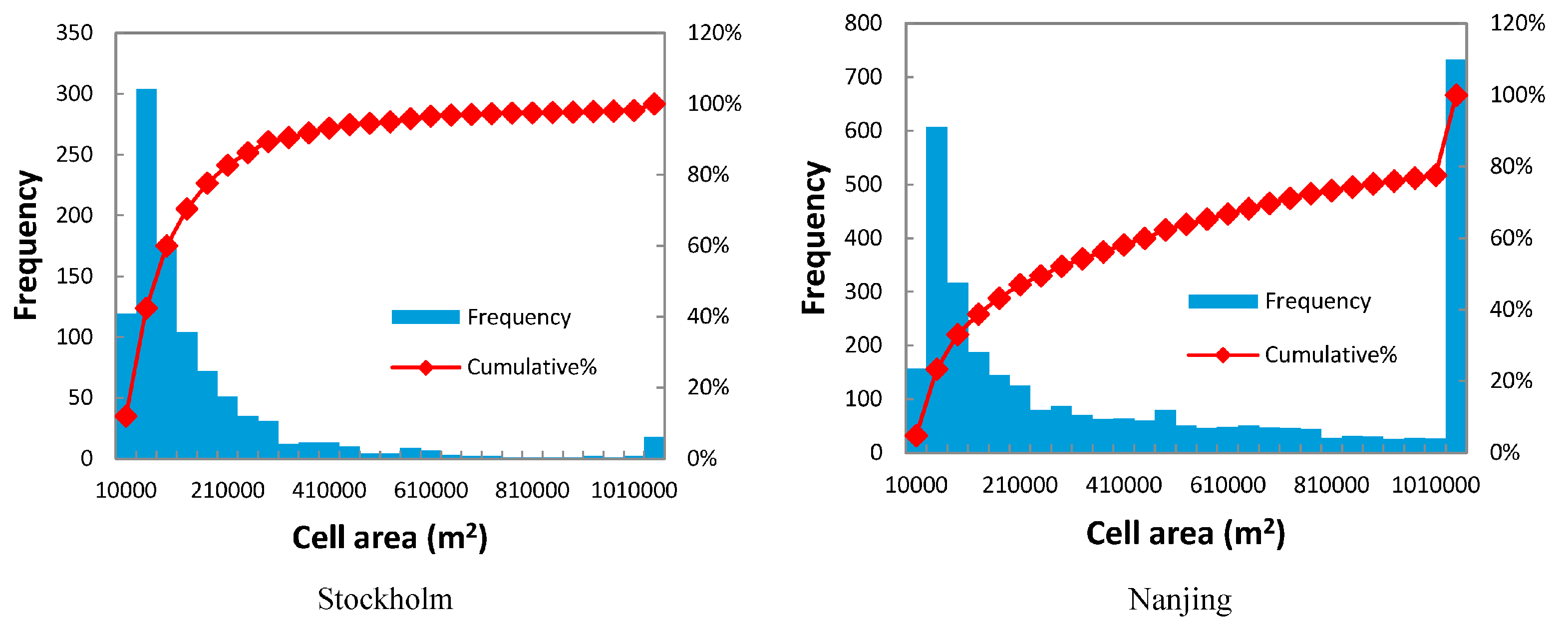
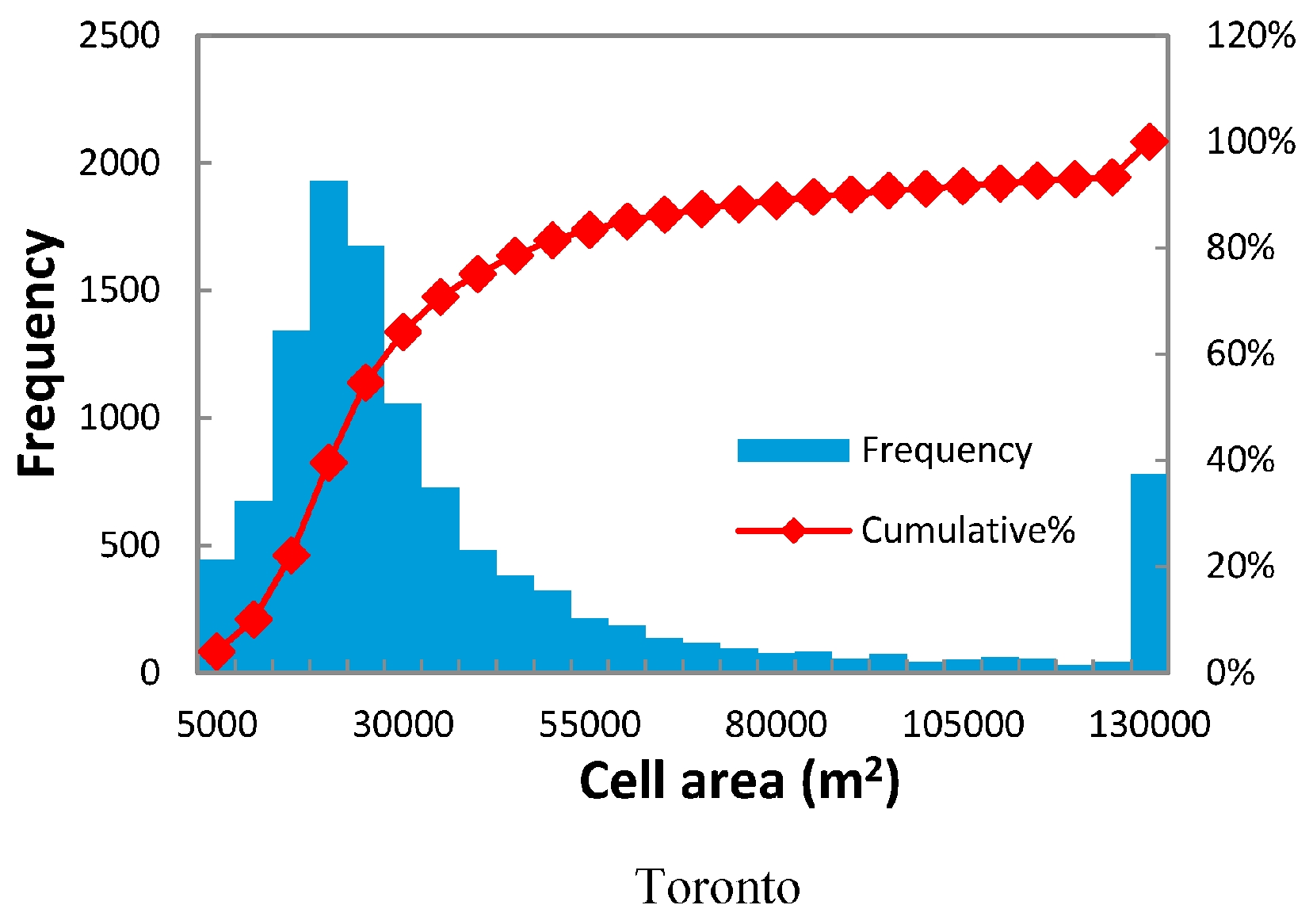
3.3. Cell Area Distribution
In planar systems, a cell is acknowledged as a closed circuit that contains at least three vertices and three edges [3]. As mentioned above, a road network appears as a two-dimensional cellular system. According to Euler’s theorem, the number of cells in a planar network C can be calculated as follows:
In the above equation, NE and NV respectively indicate the number of edges and vertices in a network. According to this formula, the values of NC for three systems can be calculated as NCSt = 992; NCNa = 3155; and NCTo = 10,031.
To better capture the underlying mechanisms of the cellular structure of the three systems and make comparisons in terms of their urban patterns, we calculated the cell areas and illustrated the distribution histograms in Figure 3. Clearly, three subplots show significant differences. It is worth noting that the figures focus on the distribution of the cell area, which is no greater than 1 km2 in the three systems. Stockholm and Nanjing present similar patterns for the small- and medium-sized cells, which can reveal the heterogeneity in the self-organized systems. However, Nanjing has a significant portion of large-sized cells because the study area covers some suburbs in which the road density is relatively low. Comparatively, the strictly-planned city of Toronto presents a single peak distribution. In this network, 90% of the cells are smaller than 0.09 km2, and 71.5% of the cell areas are located between 0.01 km2 and 0.05 km2, which is the peak of the plot.
4. Centrality of the Urban Street Networks
The complex network theory provides a novel way to explore the physical networks in our real world. We will discuss the results of main centrality distributions in this section to better capture and compare the underlying topological mechanisms of these three cities.
4.1. Degree Distribution
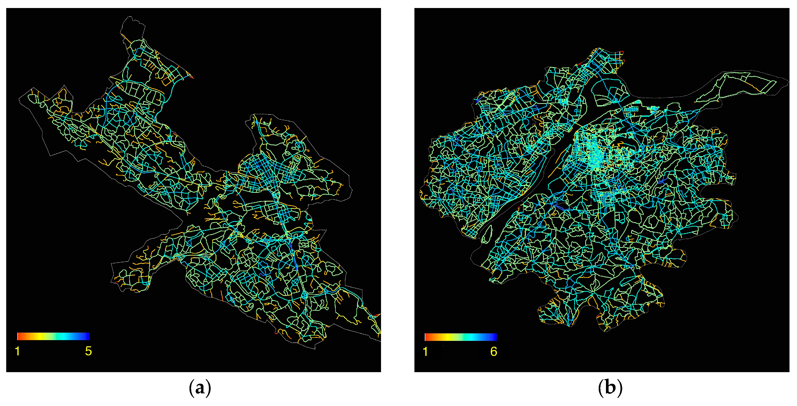
Node degree is the most fundamental and straightforward measure to quantify the connectivity of a real network. There is no difference between these three systems from an overall perspective (Figure 4). The average degrees of the street networks of Stockholm, Nanjing, and Toronto, respectively, are 2.75, 3, and 2.79. It is easy to understand, considering that intersections and ends are taken as nodes in this study. The maximum degree value is 6 because a complicated structure will decrease the efficiency of the whole system. Note that the degree value of 6 is not a theoretical maximum. A degree greater than six means there are more than three streets intersecting with each other, which is uncommon and inefficient in the real world. On the other hand, the smallest degree value is 1 for ending nodes.
4.2. Closeness Distribution
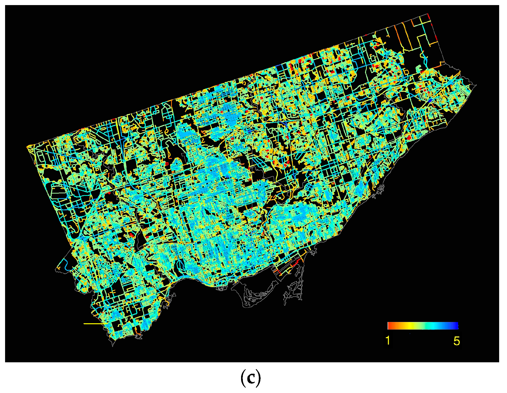
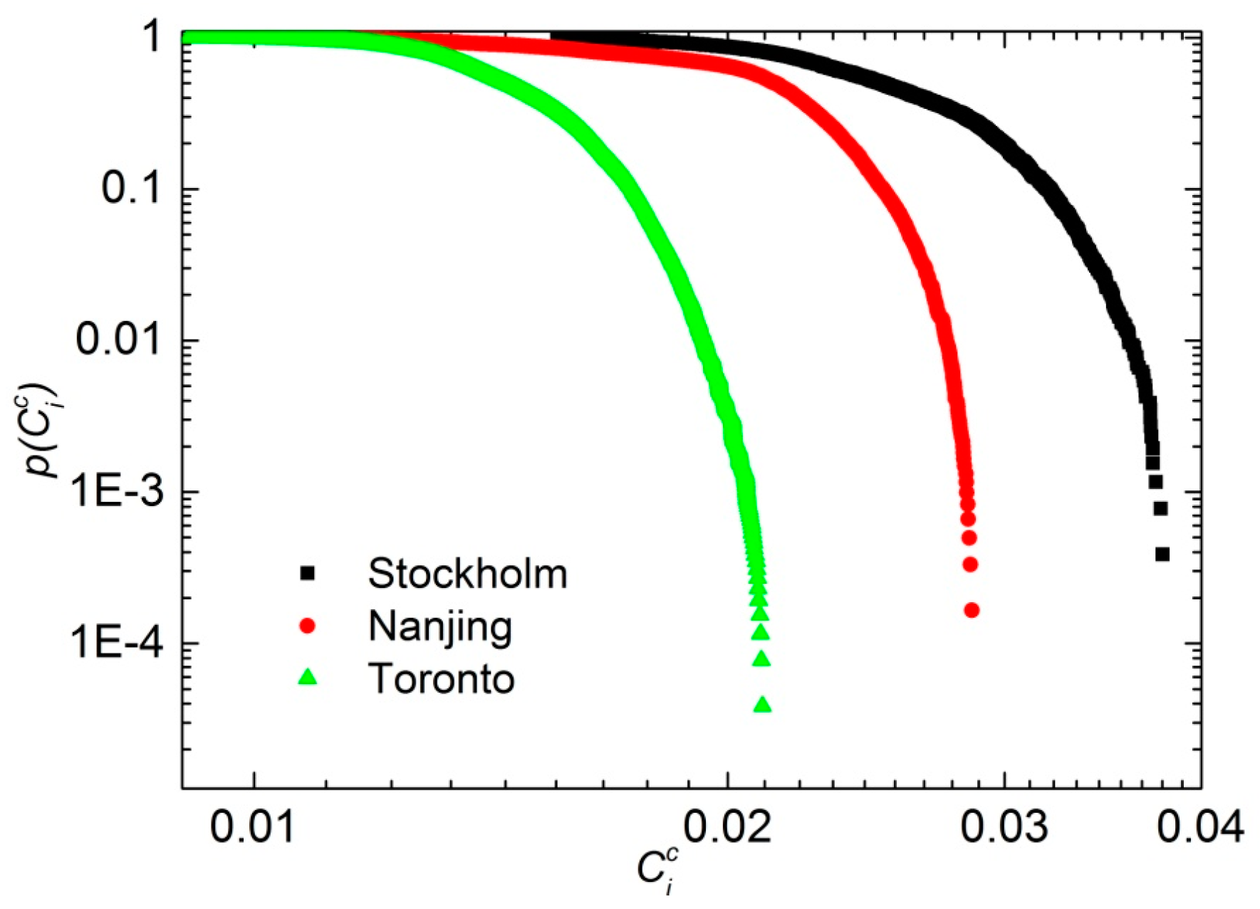
Closeness reveals the level of traveling convenience of the nodes in a system. In the real world, the distribution pattern of closeness centrality can delineate the most accessible area in a network. To depict the relationship between the closeness and other urban features, we first plot the cumulative distribution of centrality in a log-log plot for three networks (Figure 5). Remarkably, these three cities present a heavy-tailed distribution instead of a standard power law. It is a distribution with approximately two regimes, which can be divided based on a threshold value of CiC. The threshold value is decreasing while the size of the network is growing. For self-organized cities, like Stockholm and Nanjing, it indicates that there are some dominant streets with the highest closeness values, whereas a large number of streets possess low values. In contrast, Toronto presents a more even distribution. The average closeness decreases while the size increases, which are 0.025 for Stockholm, 0.02 for Nanjing, and 0.014 for Toronto. From the spatial perspective, the most central areas present the highest closeness values (Figure 6). As to the city of Nanjing, the most accessible areas are in the upper east area rather than the spatial center of the city. This area covers the Gulou, Qinhuai, Xuanwu, and part of the Jianye districts, which are the urban socio-economic centers in the real world. To summarize, compared to the two self-organized cities, the strictly planned city (i.e., Toronto), presents a better accessibility pattern from an overall perspective.
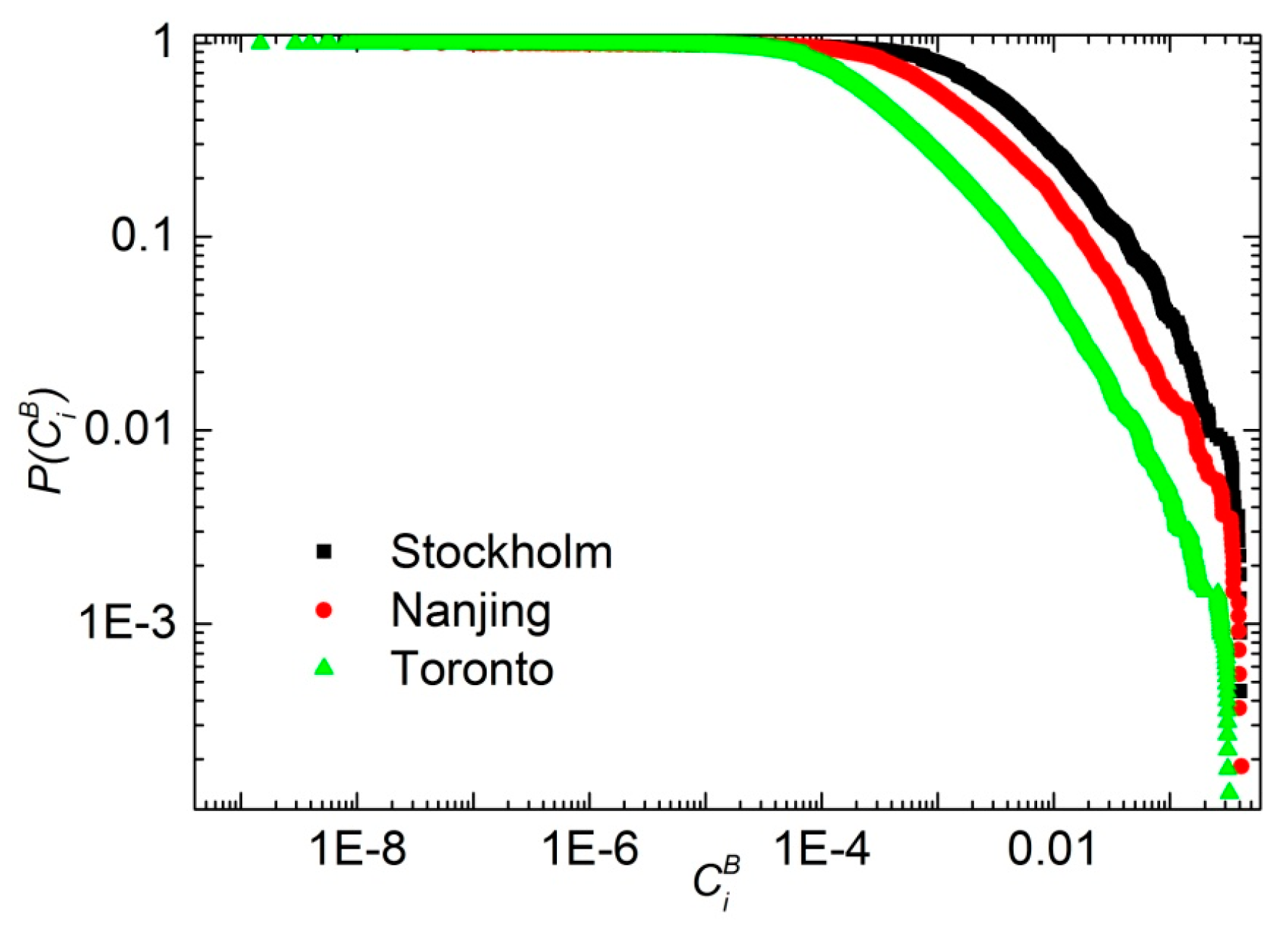
4.3. Betweenness Distribution
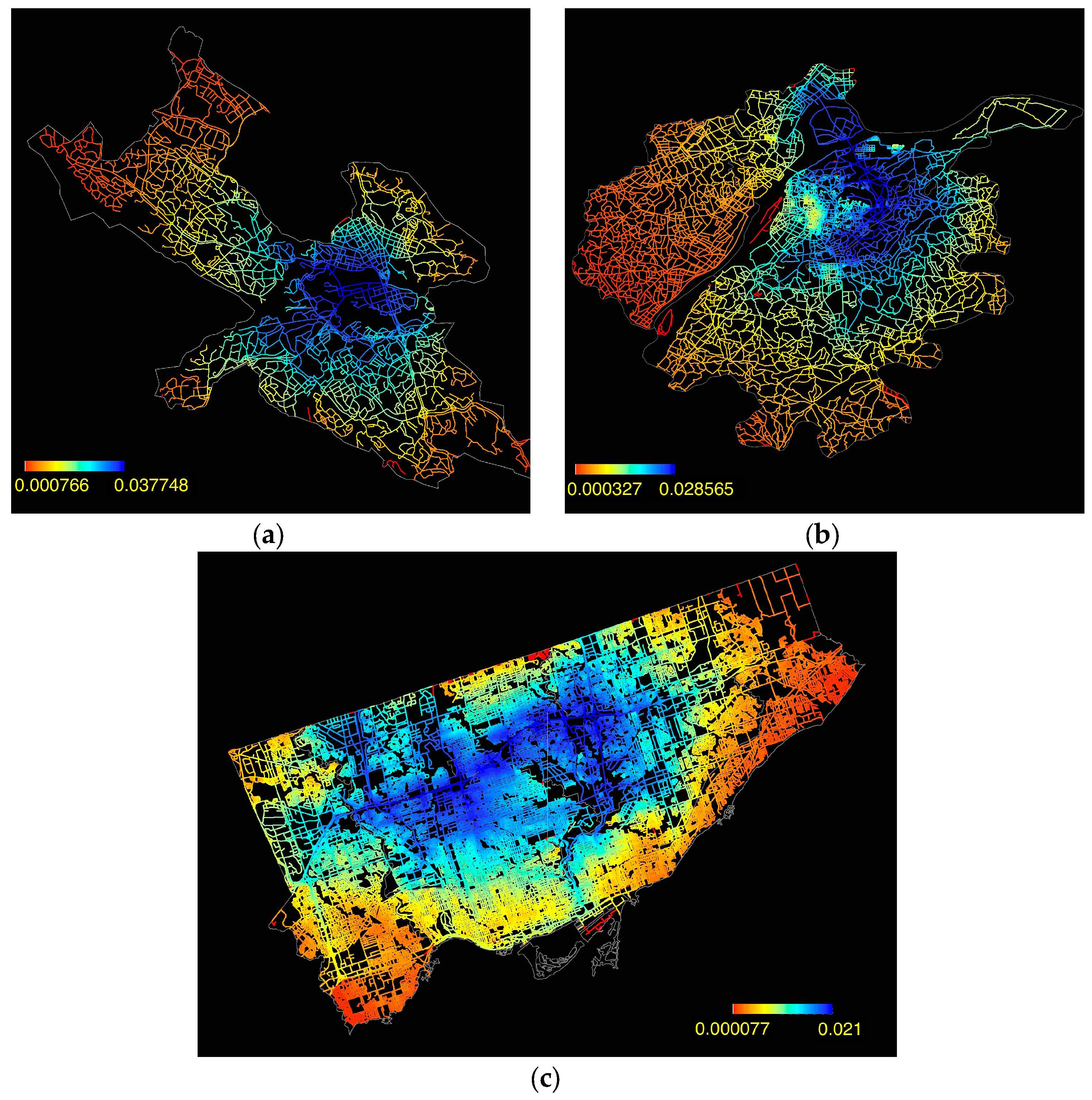
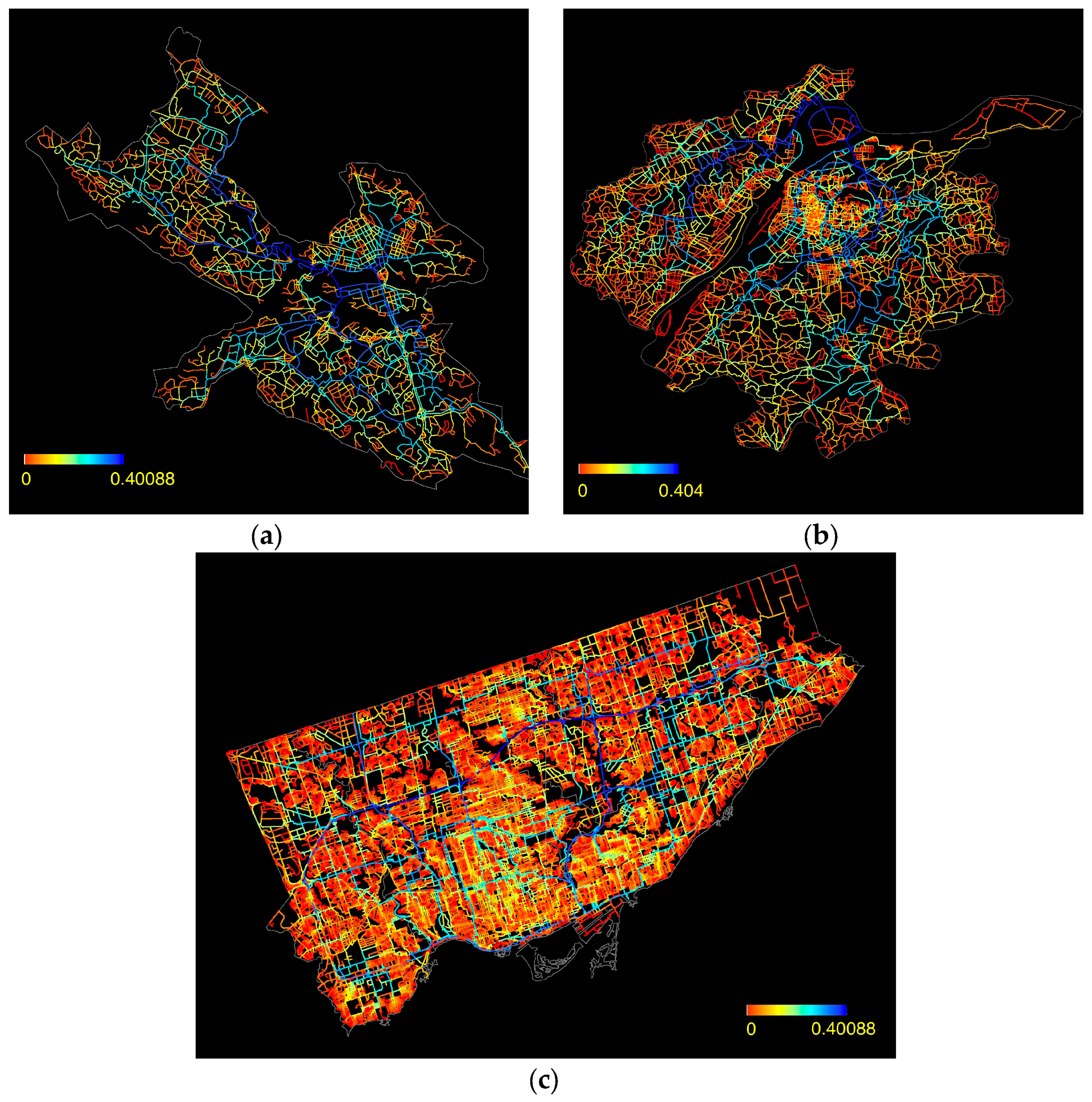
The cumulative probability distribution of betweenness centrality for the street systems of Stockholm, Nanjing, and Toronto are illustrated in Figure 7. Unlike the two-regime power-law distribution for airline systems [16,22,28,31,33], these three street networks consistently present a scaling law. It indicates that some routes or streets play the most bridging roles in the networks. In this sense, we can expect that the streets with the biggest values of betweenness centrality should be the busiest ones in the real world. This assumption is verified by our findings. In Figure 8, the bluest streets have the largest values of betweenness, and these streets construct the basic skeletons of cities. For example, in the upper left of the subplot of Stockholm, the two bluest lines are the county roads 275 and 279, respectively. These two roads connect central Stockholm with some important suburbs, such as Kista, Bromma, and Sollentuna. Additionally, both ends of these roads are connected to the European route E4, which passes from north to south through Sweden from the Finland border.
It is worth pointing out that there is a distinct difference between self-organized cities and strictly-planned cities in terms of the spatial pattern of the betweenness centrality. From Figure 8, the city of Stockholm and Nanjing both present a clear heterogeneity, whereas the city of Toronto does not. The betweenness centrality can be used to evaluate the efficiency of the whole network. Due to the probability that a node is passed by the shortest paths between all node pairs in the network, it is believed that an even distribution of the betweenness means it is a robust system that presents a high tolerance for deliberate attacks on some critical nodes [16]. In this sense, a strictly-planned city has a more optimal structure, which possesses a higher overall efficiency in traffic distribution as a consequence.
5. Conclusions
In this paper, we explored the topological structure of street systems of three cities—Stockholm, Nanjing, and Toronto—from a comparative perspective, which is of paramount importance for city planning and policy-making. From the perspective of city evolution, three cities (i.e., Stockholm, Nanjing, and Toronto) can be seen as a small-sized self-organized city, a middle-sized self-organized city, and a large-sized planned city. They present distinct planar characteristics. For example, the segment length and cell area of Toronto can be captured by a peaked distribution; in contrast, the self-organized cities share a more heterogeneous structure.
Additionally, our studies show that the centrality analyses almost pick out the real hierarchy of roads in the three systems; however, some differences appear among them. The distribution of betweenness can be seen as a useful way to measure the traffic efficiency at the global level, which depicts the difference among different city structures. To sum up, the strictly-planned city is more efficient in accessibility and connectivity based on the centrality analysis. A recommendation derived from this study for urban planners and transport engineers is that various centrality measures could be helpful in quantitative ways to evaluate city development patterns.
We have to say that this work is just a preliminary study regarding the relation between network structure and city form, and there is still work ahead. In this study, the treating of the street networks as a planar network is an approximation to the real-world scenarios. How to better describe the complexity of road networks could be a challenging subject to be discussed. Another interesting topic is adding an evolutional perspective. Considering the difficulty in acquiring the long-term historic data for street systems, constructing a simulation model will be the first step in our future work. Additionally, to make the research more systematic, we will introduce more sample cities to explore the relationships between network measures and city attributes.
Author Contributions
J.L. developed the method, collected and analyzed the data, and wrote the paper. Y.B. contributed to the related work and improved the conception and analysis.
Conflicts of Interest
The authors declare no conflict of interest.
References
- Garrison, W.; Marble, D. The Structure of Transportation Network; The Transportation Center, Northwestern University: Chicago, IL, USA, 1962. [Google Scholar]
- Kansky, K. Structure of Transportation Networks; University of Chicago Press: Chicago, IL, USA, 1963. [Google Scholar]
- Haggett, P.; Chorley, R.J. Network Analysis in Geography; Edward Arnold: London, UK, 1969. [Google Scholar]
- Xie, F.; Levinson, D. Measuring the structure of road networks. Geogr. Anal. 2007, 39, 336–356. [Google Scholar] [CrossRef]
- Xie, F.; Levinson, D. Evolving Transportation Networks; Springer: New York, NY, USA, 2011. [Google Scholar]
- Levinson, D. Network structure and city size. PLoS ONE 2012, 7, e29721. [Google Scholar] [CrossRef] [PubMed]
- Jiang, B.; Claramunt, C. Integration of space syntax into GIS: New perspectives for urban morphology. Trans. GIS 2002, 6, 295–309. [Google Scholar] [CrossRef]
- Masucci, A.P.; Stanilov, K.; Batty, M. Limited urban growth: London’s street network dynamics since the 18th century. PLoS ONE 2013, 8, e69469. [Google Scholar] [CrossRef] [PubMed]
- Newell, G.F. Traffic Flow on Transportation Networks; MIT Press: Cambridge, MA, USA, 1980. [Google Scholar]
- Xie, F.; Levinson, D. Topological evolution of surface transportation networks. Comput. Environ. Urban Syst. 2009, 33, 211–223. [Google Scholar] [CrossRef]
- Jiang, B. Topological analysis of urban street networks. Environ. Plan. B Plan. Des. 2004, 31, 151–162. [Google Scholar] [CrossRef]
- Cardillo, A.; Scellato, S.; Latora, V.; Porta, S. Structural properties of planar graphs of urban street patterns. Phys. Rev. E 2006, 73, 066107. [Google Scholar] [CrossRef] [PubMed]
- Lammer, S.; Gehlsen, B.; Helbing, D. Scaling laws in the spatial structure of urban road networks. Physica A 2006, 361, 89–95. [Google Scholar] [CrossRef]
- Jiang, B. A topological pattern of urban street networks: Universality and peculiarity. Physica A 2007, 384, 647–655. [Google Scholar] [CrossRef] [Green Version]
- Porta, S.; Strano, E.; Iacoviello, V.; Messora, R.; Latora, V.; Cardillo, A.; Wang, F.H.; Scellato, S. Street Centrality and Densities of Retail and Services in Bologna, Italy. Environ. Plan. B Plan. Des. 2009, 36, 450–465. [Google Scholar] [CrossRef]
- Lin, J.Y.; Ban, Y.F. Complex network topology of transportation systems. Transp. Rev. 2013, 33, 658–685. [Google Scholar] [CrossRef]
- Scellato, S.; Cardillo, A.; Latora, V.; Porta, S. The backbone of a city. Eur. Phys. J. B 2006, 50, 221–225. [Google Scholar] [CrossRef]
- Barthélemy, M.; Flammini, A. Optimal traffic networks. J. Stat. Mech. 2006, 2006, L07002. [Google Scholar] [CrossRef]
- Jiang, B.; Duan, Y.Y.; Lu, F.; Yang, T.H.; Zhao, J. Topological structure of urban street networks from the perspective of degree correlation. arXiv, 2013; arXiv:1308.1533. [Google Scholar]
- Porta, S.; Crucitti, P.; Latora, V. The network analysis of urban streets: A dual approach. Physica A 2006, 369, 853–866. [Google Scholar] [CrossRef]
- Porta, S.; Crucitti, P.; Latora, V. The network analysis of urban streets: A primal approach. Environ. Plan. B Plan. Des. 2006, 33, 705–725. [Google Scholar] [CrossRef]
- Guimera, R.; Mossa, S.; Turtschi, A.; Amaral, L.A.N. The worldwide air transportation network: Anomalous centrality, community structure, and cities’ global roles. Proc. Natl. Acad. Sci. USA 2005, 102, 7794–7799. [Google Scholar] [CrossRef] [PubMed]
- Lee, K.; Jung, W.S.; Park, J.S.; Choi, M.Y. Statistical analysis of the Metropolitan Seoul Subway System: Network and passengers flows. Physica A 2008, 387, 6231–6234. [Google Scholar] [CrossRef]
- Lu, H.P.; Shi, Y. Complexity of public transport network. Tsinghua Sci. Technol. 2007, 12, 204–213. [Google Scholar] [CrossRef]
- Sienkiewicz, J.; Holyst, J.A. Statistical analyses of 22 public transport networks in Poland. Phys. Rev. E 2005, 72, 046127. [Google Scholar] [CrossRef] [PubMed]
- Ferber, C.V.; Holovatch, T.; Holovatch, Y.; Palchykov, V. Public transportnetworks: Empirical and modeling. Eur. Phys. J. B 2009, 68, 261–275. [Google Scholar] [CrossRef]
- Li, W.; Cai, X. Statistical analysis of airport network of China. Phys. Rev. E 2004, 69, 046106. [Google Scholar] [CrossRef] [PubMed]
- Liu, H.T.; Zhou, T. Empirical study of China city airline network. Acta Phys. Sin. 2007, 56, 106–112. (In Chinese) [Google Scholar]
- Bagler, G. Analysis of the airport network of India as a complex weighted network. Physica A 2008, 387, 2972–2980. [Google Scholar] [CrossRef]
- Xu, Z.; Harriss, R. Exploring the structure of the US intercity passenger air transportation network: A weighted complex network approach. GeoJournal 2008, 73, 87–102. [Google Scholar] [CrossRef]
- Wang, J.; Mo, H.H.; Wang, F.H.; Jin, J.F. Exploring the network structure and nodal centrality of China’s air transport network: A complex network approach. J. Transp. Geogr. 2011, 19, 712–721. [Google Scholar] [CrossRef]
- Rabasz, E.; Barabasi, A.L. Hierarchical organization in complex networks. Phys. Rev. E 2003, 67, 026112. [Google Scholar]
- Lin, J.Y. Network analysis of China’s aviation system, statistical and spatial structure. J. Transp. Geogr. 2012, 22, 109–117. [Google Scholar] [CrossRef]
- Buhl, J.; Gautrais, J.; Reeves, N.; Sole, R.V.; Valverde, S.; Kuntz, P.; Theraulaz, G. Topological patterns in street networks of self-organized urban settlements. Eur. Phys. J. B 2006, 49, 513–522. [Google Scholar] [CrossRef]
- Bureau of Sweden. Available online: http://www.scb.se (accessed on 18 July 2014).
- Statistics Canada. Available online: http://www.statcan.gc.ca (accessed on 19 July 2014).
- Map and Data Library of the University of Toronto. Available online: http://mdl.library.utoronto.ca/ (accessed on 19 July 2014).
- Diestel, R. Graph Theory; Springer-Verlag: New York, NY, USA, 2005. [Google Scholar]
- Zeng, H.L.; Guo, Y.D.; Zhu, C.P.; Mitrovic, M.; Tadic, B. Congestion patterns of traffic studied on Nanjing city dual graph. In Proceedings of the 16th International Conference on Digital Signal Processing, Santorini, Greece, 5–7 July 2009; pp. 982–989. [Google Scholar]
- Freeman, L.C. A set of measures of centrality based upon betweenness. Sociometry 1977, 40, 35–41. [Google Scholar] [CrossRef]
- Ulrik, B. A faster algorithm for betweenness centrality. J. Math. Sociol. 2001, 25, 163–177. [Google Scholar]
- Ulrik, B. On variants of shortest-path betweenness centrality and their generic computation. Soc. Netw. 2008, 30, 136–145. [Google Scholar]
- Crucitti, P.; Latora, V.; Porta, S. Centrality measures in spatial networks of urban streets. Phys. Rev. E 2006, 73, 036125. [Google Scholar] [CrossRef] [PubMed]
- Gastner, M.T.; Newman, M.E.J. The spatial structure of networks. Eur. Phys. J. B 2006, 49, 247–252. [Google Scholar] [CrossRef]
Figure 1.
Study areas of city of (a) Stockholm; (b) Nanjing; and (c) Toronto.

Figure 2.
Distance distribution histograms of urban street systems of Stockholm, Nanjing, and Toronto.
Figure 2.
Distance distribution histograms of urban street systems of Stockholm, Nanjing, and Toronto.

Figure 3.
Distribution histograms of the cell area of urban street systems of Stockholm, Nanjing, and Toronto.
Figure 3.
Distribution histograms of the cell area of urban street systems of Stockholm, Nanjing, and Toronto.


Figure 4.
Degree distributions of the urban street systems of (a) Stockholm; (b) Nanjing, and (c) Toronto (the values of degree centrality are divided into 10 classes from the minimum to the maximum, corresponding to the color from red to blue).
Figure 4.
Degree distributions of the urban street systems of (a) Stockholm; (b) Nanjing, and (c) Toronto (the values of degree centrality are divided into 10 classes from the minimum to the maximum, corresponding to the color from red to blue).


Figure 5.
Cumulative probability distributions of closeness centrality of: Stockholm, Nanjing and Toronto.
Figure 5.
Cumulative probability distributions of closeness centrality of: Stockholm, Nanjing and Toronto.

Figure 6.
Closeness distributions of the urban street systems of (a) Stockholm; (b) Nanjing, and (c) Toronto (the values of closeness centrality are divided into 32 classes from the minimum to the maximum, corresponding to the color from red to blue).
Figure 6.
Closeness distributions of the urban street systems of (a) Stockholm; (b) Nanjing, and (c) Toronto (the values of closeness centrality are divided into 32 classes from the minimum to the maximum, corresponding to the color from red to blue).

Figure 7.
Cumulative probability distributions of betweenness centrality of: Stockholm, Nanjing, and Toronto.
Figure 7.
Cumulative probability distributions of betweenness centrality of: Stockholm, Nanjing, and Toronto.

Figure 8.
Betweenness distributions of the urban street systems of (a) Stockholm; (b) Nanjing, and (c) Toronto (the values of betweenness centrality are divided into 32 classes from the minimum to the maximum, corresponding to the color from red to blue).
Figure 8.
Betweenness distributions of the urban street systems of (a) Stockholm; (b) Nanjing, and (c) Toronto (the values of betweenness centrality are divided into 32 classes from the minimum to the maximum, corresponding to the color from red to blue).


Table 1.
Basic statistics of three cities in 2012.
| City | Population | Area (km2) | Population Density (per/km2) | GDP ($bil) | Mean Income ($) |
|---|---|---|---|---|---|
| Stockholm | 881,235 | 188 | 4687 | 34.5 | 48,780 |
| Nanjing | 6,376,500 | 3098 | 7573 | 59.5 | 5906 |
| Toronto | 2,791,140 | 630 | 4430 | 143.8 | 42,736 |
Table 2.
Basic planar statistics of three cities.
| Name | NV | NE | Ltotal (km) | cc | Lgeo | α | β | γ | Ρ (km/km2) |
|---|---|---|---|---|---|---|---|---|---|
| Stockholm | 2612 | 3603 | 971.3 | 0.052 | 40 | 0.190 | 1.379 | 0.460 | 5.17 |
| Nanjing | 6121 | 9275 | 6219.9 | 0.070 | 50.2 | 0.258 | 1.515 | 0.505 | 7.39 |
| Toronto | 26093 | 37123 | 5650 | 0.041 | 69.6 | 0.211 | 1.423 | 0.474 | 8.97 |
Note: NV and NE respectively indicate the number of nodes and edges of the network, Ltotal is the total length of the streets; cc represents clustering coefficient of the network; Lgeo is the characteristic length path of the network and P calculates the road network density.
© 2017 by the authors. Licensee MDPI, Basel, Switzerland. This article is an open access article distributed under the terms and conditions of the Creative Commons Attribution (CC BY) license (http://creativecommons.org/licenses/by/4.0/).
Share and Cite
MDPI and ACS Style
Lin, J.; Ban, Y. Comparative Analysis on Topological Structures of Urban Street Networks. ISPRS Int. J. Geo-Inf. 2017, 6, 295. https://0-doi-org.brum.beds.ac.uk/10.3390/ijgi6100295
AMA Style
Lin J, Ban Y. Comparative Analysis on Topological Structures of Urban Street Networks. ISPRS International Journal of Geo-Information. 2017; 6(10):295. https://0-doi-org.brum.beds.ac.uk/10.3390/ijgi6100295
Chicago/Turabian StyleLin, Jingyi, and Yifang Ban. 2017. "Comparative Analysis on Topological Structures of Urban Street Networks" ISPRS International Journal of Geo-Information 6, no. 10: 295. https://0-doi-org.brum.beds.ac.uk/10.3390/ijgi6100295
Note that from the first issue of 2016, this journal uses article numbers instead of page numbers. See further details here.