A New Recursive Filtering Method of Terrestrial Laser Scanning Data to Preserve Ground Surface Information in Steep-Slope Areas

Abstract
:1. Introduction
2. Research Areas and Datasets
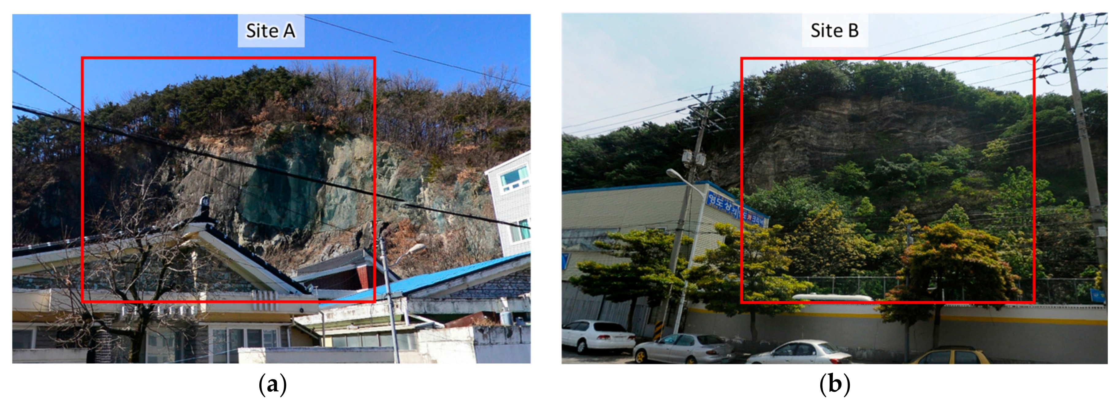
2.1. Study Area
2.2. Data Description
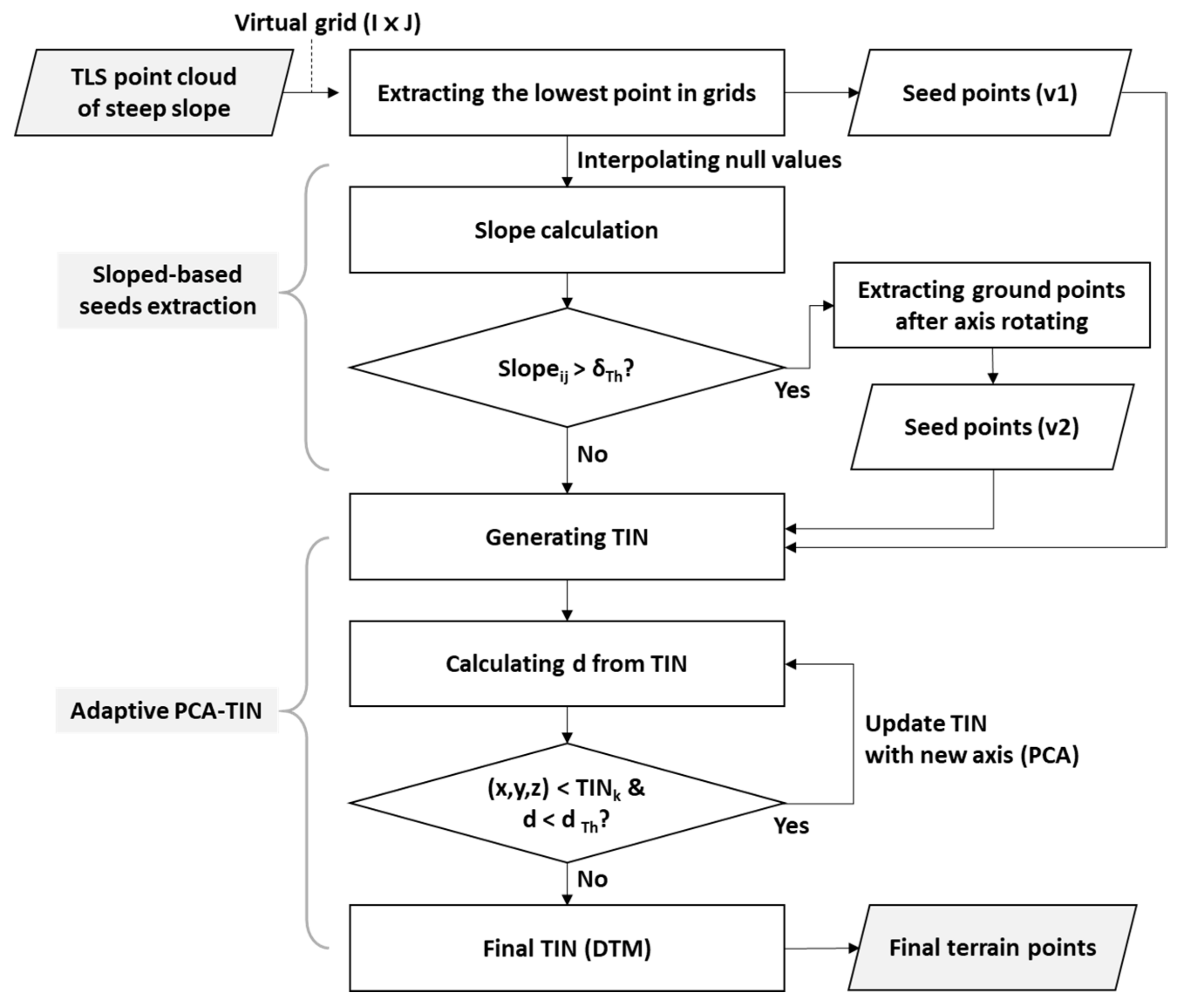
3. Recursive Filtering Method
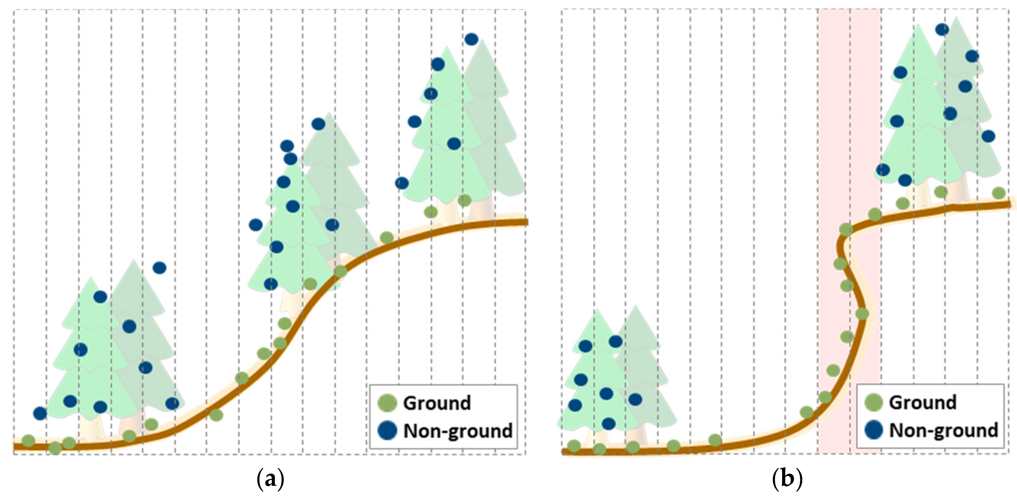
3.1. Slope-Based Seed Points Extraction
3.1.1. Extracting the Lowest Point
3.1.2. Slope Angle Calculation
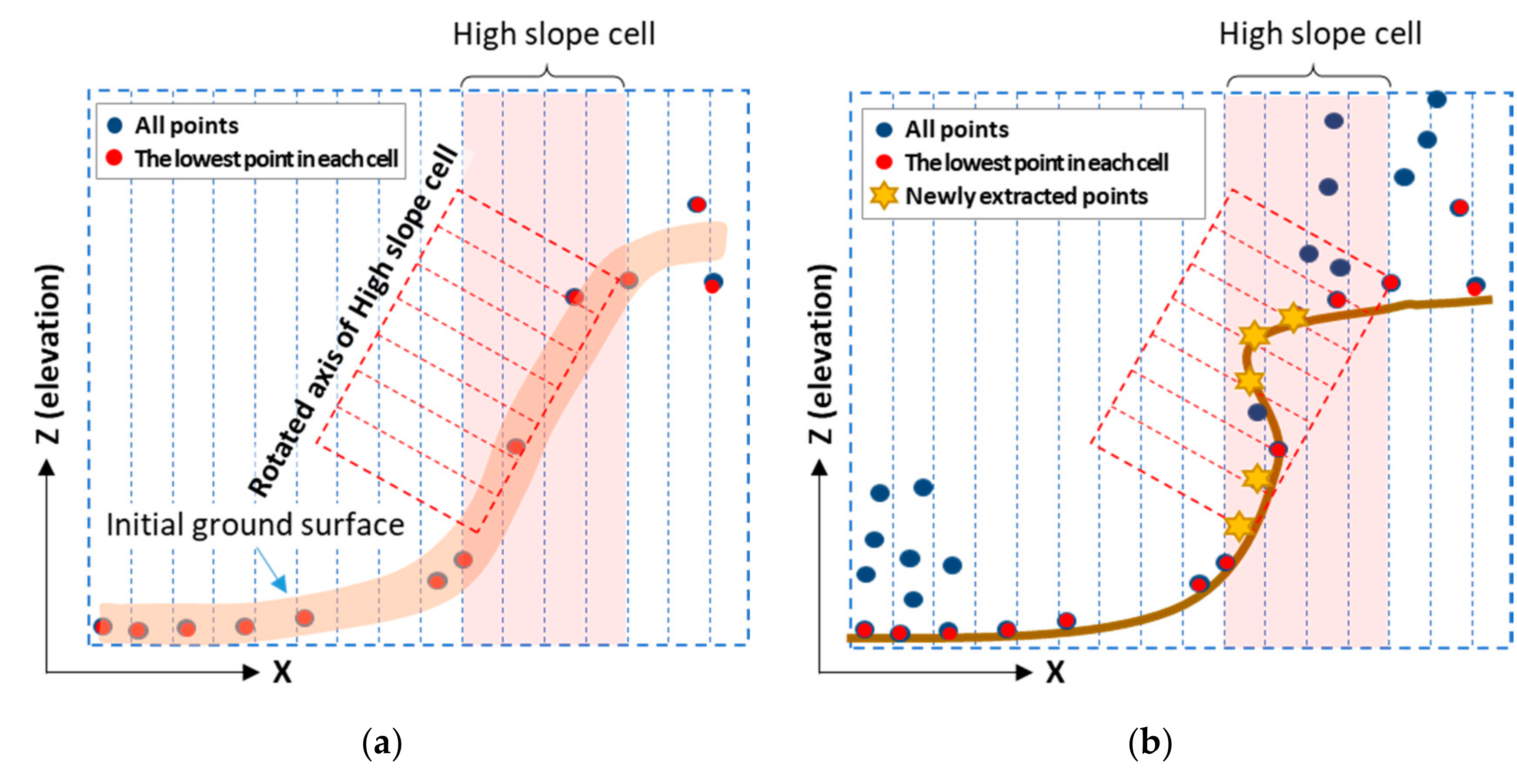
3.1.3. Extracting Ground Points after Axis Rotation
3.2. Adaptive PCA-TIN
3.2.1. Initial TIN after Rotating the Axis
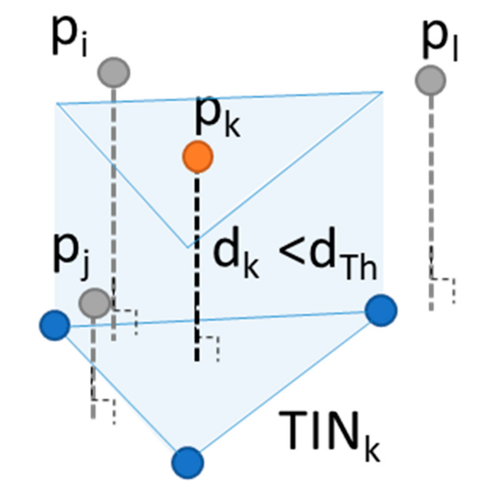
3.2.2. Adding Points for the Next TIN
3.2.3. Reconstructing TIN with New Axis (PCA)
3.3. Accuracy Assessment
4. Results and Discussion
5. Conclusions
Acknowledgments
Author Contributions
Conflicts of Interest
References
- Cruden, D.M. A simple definition of a landslide. Bull. Int. Assoc. Eng. Geol. 1991, 43, 27–29. [Google Scholar] [CrossRef]
- Schuster, R.L.; Highland, L.M. Impact of landslides and innovative landslide-mitigation measures on the natural environment. In Proceedings of the International Conference on Slope Engineering, Hong Kong, China, 7–10 December 2003. [Google Scholar]
- Kechebour, B.E.L. Relation between Stability of Slope and the Urban Density: Case Study. Procedia Eng. 2015, 114, 824–831. [Google Scholar] [CrossRef]
- BBC. China Landslide: 15 Dead, over 100 Missing in Sichuan. BBC News. 24 June 2017. Available online: http://www.bbc.com/news/world-asia-china-40390642 (accessed on 23 August 2017).
- BBC. Sierra Leone Floods Kill Hundreds as Mudslides Bury Houses. BBC News. BBC News. 15 August 2017. Available online: http://www.bbc.com/news/world-africa-40926187 (accessed on 23 August 2017).
- Suk, G.-H. Seoul Faces Increasing Risk of Landslides. The Korea Herald. 18 July 2013. Available online: http://www.koreaherald.com/view.php?ud=20130718000703 (accessed on 23 August 2017).
- Cho, H.-A. Woomyunsan Landslide, Two Missing Persons Found…18 People Died. NEWSIS. 28 July 2011. Available online: http://www.newsis.com/view/?id=NISX20110728_0008810252 (accessed on 23 August 2017).
- Aleotti, P.; Chowdhury, R. Landslide hazard assessment: Summary review and new perspectives. Bull. Eng. Geol. Environ. 1999, 58, 21–44. [Google Scholar] [CrossRef]
- Baek, M.H.; Kim, T.H. A study on the use of planarity for quick identification of potential landslide hazard. Nat. Hazards Earth Syst. Sci. 2015, 15, 997–1009. [Google Scholar] [CrossRef]
- Hess, D.M.; Leshchinsky, B.A.; Bunn, M.; Benjamin Mason, H.; Olsen, M.J. A simplified three-dimensional shallow landslide susceptibility framework considering topography and seismicity. Landslides 2017, 14, 1677–1697. [Google Scholar] [CrossRef]
- Pradhan, B.M.; Mansor, S.; Pirasteh, S.; Buchroithner, M.F. Landslide hazard and risk analyses at a landslide prone catchment area using statistical based geospatial model. Int. J. Remote Sens. 2011, 32, 4075–4087. [Google Scholar] [CrossRef]
- Rawat, M.S.; Joshi, V.; Rawat, B.S.; Kumar, K. Landslide movement monitoring using GPS technology: A case study of Bakthang landslide, Gangtok, East Sikkim, India. J. Dev. Agric. Econ. 2011, 3, 194–200. [Google Scholar]
- Lee, S.; Chwae, U.; Min, K. Landslide susceptibility mapping by correlation between topography and geological structure: The Janghung area, Korea. Geomorphology 2002, 46, 149–162. [Google Scholar] [CrossRef]
- Lee, S.; Lee, M.-J.; Jung, H.-S. Data Mining Approaches for Landslide Susceptibility Mapping in Umyeonsan, Seoul, South Korea. Appl. Sci. 2017, 7, 683. [Google Scholar] [CrossRef]
- Glennie, C.L.; Carter, W.E.; Shrestha, R.L.; Dietrich, W.E. Geodetic imaging with airborne LiDAR: The Earth’s surface revealed. Rep. Prog. Phys. 2013, 76, 086801. [Google Scholar] [CrossRef] [PubMed]
- Telling, J.; Lyda, A.; Hartzell, P.; Glennie, C. Review of Earth science research using terrestrial laser scanning. Earth-Sci. Rev. 2017, 169, 35–68. [Google Scholar] [CrossRef]
- Kashani, A.; Olsen, M.; Parrish, C.; Wilson, N. A Review of LIDAR Radiometric Processing: From Ad Hoc Intensity Correction to Rigorous Radiometric Calibration. Sensors 2015, 15, 28099. [Google Scholar] [CrossRef] [PubMed]
- Young, A.P.; Olsen, M.J.; Driscoll, N.; Rick, R.E.; Gutierrez, R.; Guza, R.T.; Johnstone, E.; Kuester, F. Comparison of airborne and terrestrial lidar estimates of seacliff erosion in Southern California. ISPRS J. Photogram. Eng. Remote Sens. 2010, 76, 421–427. [Google Scholar] [CrossRef]
- Rodríguez-Caballero, E.; Afana, A.; Chamizo, S.; Solé-Benet, A.; Canton, Y. A new adaptive method to filter terrestrial laser scanner point clouds using morphological filters and spectral information to conserve surface micro-topography. ISPRS J. Photogramm. Remote Sens. 2016, 117, 141–148. [Google Scholar] [CrossRef]
- Pirasteh, S.; Li, J. Landslides investigations from geoinformatics perspective: quality, challenges, and recommendations. Geomat. Nat. Hazards Risk 2016, 1–18. [Google Scholar] [CrossRef]
- Guan, H.; Li, J.; Yu, Y.; Zhong, L.; Ji, Z. DEM generation from lidar data in wooded mountain areas by cross-section-plane analysis. Int. J. Remote Sens. 2014, 35, 927–948. [Google Scholar] [CrossRef]
- Liu, X. Airborne LiDAR for DEM generation: Some critical issues. Prog. Phys. Geogr. 2008, 32, 31–49. [Google Scholar]
- Mongus, D.; Žalik, B. Parameter-free ground filtering of LiDAR data for automatic DTM generation. ISPRS J. Photogramm. Remote Sens. 2012, 67, 1–12. [Google Scholar] [CrossRef]
- Kobler, A.; Pfeifer, N.; Ogrinc, P.; Todorovski, L.; Oštir, K.; Džeroski, S. Repetitive interpolation: A robust algorithm for DTM generation from Aerial Laser Scanner Data in forested Terrain. Remote Sens. Environ. 2007, 108, 9–23. [Google Scholar] [CrossRef]
- Axelsson, P. DEM generation from laser scanner data using adaptive TIN models. Int. Arch. Photogramm. Remote Sens. 2000, XXXIII, 340–346. [Google Scholar]
- Evans, J.S.; Hudak, A.T. A multiscale curvature algorithm for classifying discrete return LiDAR in forested environments. IEEE Trans. Geosci. Remote Sens. 2007, 45, 1029–1038. [Google Scholar] [CrossRef]
- Gallay, M. Direct acquisition of data: Airborne laser scanning. In Geomorphological Techniques; British Society for Geomorphology: London, UK, 2013; pp. 1–17. [Google Scholar]
- Vosselman, G. Slope based filtering of laser altimetry data. Int. Arch. Photogramm. Remote Sens. 2000, XXXIII, 935–942. [Google Scholar]
- Yunfei, B.; Guoping, L.; Chunxiang, C.; Xiaowen, L.; Hao, Z.; Qisheng, H.; Linyan, B.; Chaoyi, C. Classification of LIDAR point cloud and generation of DTM from LIDAR height and intensity data in forested area. Int. Arch. Photogram. Remote Sens. Spat. Inf. Sci. 2008, XXXVII, 313–318. [Google Scholar]
- Meng, X.; Currit, N.; Zhao, K. Ground Filtering Algorithms for Airborne LiDAR Data: A Review of Critical Issues. Remote Sens. 2010, 2, 833. [Google Scholar] [CrossRef]
- Chen, Z.; Gao, B.; Devereux, B. State-of-the-art: DTM generation using airborne LIDAR data. Sensors 2017, 17, 150. [Google Scholar] [CrossRef] [PubMed]
- Li, Y.; Yong, B.; Wu, H.; An, R.; Xu, H.; Xu, J.; He, Q. Filtering Airborne Lidar Data by Modified White Top-Hat Transform with Directional Edge Constraints. Photogramm. Eng. Remote Sens. 2014, 80, 133–141. [Google Scholar] [CrossRef]
- Mongus, D.; Lukač, N.; Žalik, B. Ground and building extraction from LiDAR data based on differential morphological profiles and locally fitted surfaces. ISPRS J. Photogramm. Remote Sens. 2014, 93, 145–156. [Google Scholar] [CrossRef]
- Sithole, G.; Vosselman, G. Experimental comparison of filter algorithms for bare-Earth extraction from airborne laser scanning point clouds. ISPRS J. Photogramm. Remote Sens. 2004, 59, 85–101. [Google Scholar] [CrossRef]
- Chen, C.; Li, Y.; Yan, C.; Dai, H.; Liu, G.; Guo, J. An improved multi-resolution hierarchical classification method based on robust segmentation for filtering ALS point clouds. Int. J. Remote Sens. 2016, 37, 950–968. [Google Scholar] [CrossRef]
- Sithole, G. Filtering of laser altimetry data using a slope adaptive filter. Int. Arch. Photogramm. Remote Sens. 2001, 34, 203–210. [Google Scholar]
- Chen, Q.; Gong, P.; Baldocchi, D.; Xie, G. Filtering airborne laser scanning data with morphological methods. Photogramm. Eng. Remote Sens. 2007, 73, 175–185. [Google Scholar] [CrossRef]
- Zhang, K.; Chen, S.C.; Whitman, D.; Shyu, M.L.; Yan, J.; Zhang, C. A progressive morphological filter for removing nonground measurements from airborne LIDAR data. IEEE Trans. Geosci. Remote Sens. 2003, 41, 872–882. [Google Scholar] [CrossRef]
- Błaszczak-Bąk, W.; Janowski, A.; Kamiński, W.; Rapiński, J. Application of the Msplit method for filtering airborne laser scanning data-sets to estimate digital terrain models. Int. J. Remote Sens. 2015, 36, 2421–2437. [Google Scholar] [CrossRef]
- Kraus, K.; Pfeifer, N. Determination of terrain models in wooded areas with airborne laser scanner data. ISPRS J. Photogramm. Remote Sens. 1998, 53, 193–203. [Google Scholar] [CrossRef]
- Rapinski, J.; Kaminski, W.; Janowski, A.; Blaszczak-Bak, W. ALS Data Filtration with Fuzzy Logic. J. Indian Soc. Remote Sens. 2011, 39, 591–597. [Google Scholar] [CrossRef]
- Wasowski, J.; Bovenga, F. Remote sensing of landslide motion with emphasis on satellite multitemporal interferometry applications: an overview. In Landslide Hazards, Risks and Disasters; Academic Press: Boston, MA, USA, 2015; pp. 345–403. [Google Scholar]
- Pirotti, F.; Guarnieri, A.; Vettore, A. Ground filtering and vegetation mapping using multi-return terrestrial laser scanning. ISPRS J. Photogramm. Remote Sens. 2013, 76, 56–63. [Google Scholar] [CrossRef]
- Meng, X.; Wang, L.; Silván-Cárdenas, J.L.; Currit, N. A multi-directional ground filtering algorithm for airborne LIDAR. ISPRS J. Photogramm. Remote Sens. 2009, 64, 117–124. [Google Scholar] [CrossRef]
- Wang, C.; Menenti, M.; Stoll, M.P.; Feola, A.; Belluco, E.; Marani, M. Separation of ground and low vegetation signatures in LiDAR measurements of salt-marsh environments. IEEE Trans. Geosci. Remote Sens. 2009, 47, 2014–2023. [Google Scholar] [CrossRef]
- National Assembly. Prevention of Steep Slope Disasters Act; South Koreas National Assembly: Seoul, South Korea, 2016. [Google Scholar]
- MPSS. 2016 National Security White Paper—700-Day Footprint for the Safety of the People. MPSS: Sejong, South Korea, 2016. [Google Scholar]
- Pyun, H. ‘Crumbling’ Five-Day Specimen Inspection of Twenty-Eight Steep Slopes just before the Collapse. NEWSIS. 28 December 2016. Available online: http://www.newsis.com/ar_detail/view.html/?ar_id=NISX20160319_0013968462&cID=10201&pID=10200 (accessed on 24 September 2017).
- RIEGL. Product Detail: RIEGL VZ-2000. 2017. Available online: http://www.riegl.com/nc/products/terrestrial-scanning/produktdetail/product/scanner/45/ (accessed on 16 July 2017).
- RIEGL. Datasheet of RiSCAN PRO. 2016. Available online: http://www.riegl.com/uploads/tx_pxpriegldownloads/11_DataSheet_RiSCAN-PRO_2016-09-19.pdf (accessed on 16 July 2017).
- Kolecka, N. Vector algebra for Steep Slope Model analysis. Landf. Anal. 2012, 21, 17–25. [Google Scholar]
- Zhang, W.; Qi, J.; Wan, P.; Wang, H.; Xie, D.; Wang, X.; Yan, G. An easy-to-use airborne LiDAR data filtering method based on cloth simulation. Remote Sens. 2016, 8, 501. [Google Scholar] [CrossRef]


| Category | Number of Points | Area (m2) | Mean Slope (°) | Height (m) | ||
|---|---|---|---|---|---|---|
| Maximum | Minimum | Average | ||||
| Site A | 2,519,944 | 5252 | 36.61 | 64.85 | −1.88 | 26.16 |
| Site B | 3,966,393 | 1378 | 41.20 | 35.68 | −8.76 | 8.52 |
| Category | Number of Points | Filering Method | Extracted Points as Ground | RMSE (Root Mean Squared Error) (cm) | MBE (Mean Bias Error) (cm) | Data Missing Ratio (%) |
|---|---|---|---|---|---|---|
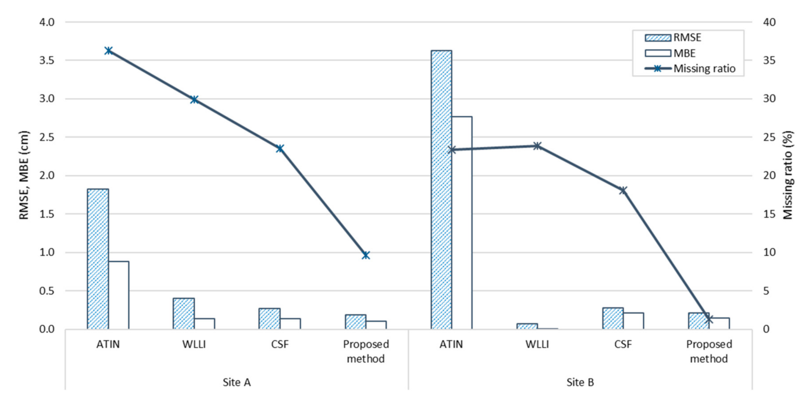
| Site A | 2,519,944 | ATIN (adaptive TIN) | 515,543 | 18.22 | 8.79 | 36.25 |
| WLLI (weighted linear least-squares interpolation-based method) | 519,321 | 4.00 | 1.34 | 29.90 | ||
| CFS (cloth simulation filter) | 595,257 | 2.72 | 1.38 | 23.51 | ||
| Proposed method | 531,077 | 1.84 | 1.07 | 9.62 | ||
| Site B | 3,966,393 | ATIN | 561,563 | 36.30 | 27.69 | 23.40 |
| WLLI | 844,003 | 0.71 | 0.08 | 23.87 | ||
| CFS | 782,799 | 2.81 | 2.09 | 18.07 | ||
| Proposed method | 553,850 | 2.13 | 1.45 | 1.25 |
© 2017 by the authors. Licensee MDPI, Basel, Switzerland. This article is an open access article distributed under the terms and conditions of the Creative Commons Attribution (CC BY) license (http://creativecommons.org/licenses/by/4.0/).
Share and Cite
Kim, M.-K.; Kim, S.; Sohn, H.-G.; Kim, N.; Park, J.-S. A New Recursive Filtering Method of Terrestrial Laser Scanning Data to Preserve Ground Surface Information in Steep-Slope Areas. ISPRS Int. J. Geo-Inf. 2017, 6, 359. https://0-doi-org.brum.beds.ac.uk/10.3390/ijgi6110359
Kim M-K, Kim S, Sohn H-G, Kim N, Park J-S. A New Recursive Filtering Method of Terrestrial Laser Scanning Data to Preserve Ground Surface Information in Steep-Slope Areas. ISPRS International Journal of Geo-Information. 2017; 6(11):359. https://0-doi-org.brum.beds.ac.uk/10.3390/ijgi6110359
Chicago/Turabian StyleKim, Mi-Kyeong, Sangpil Kim, Hong-Gyoo Sohn, Namhoon Kim, and Je-Sung Park. 2017. "A New Recursive Filtering Method of Terrestrial Laser Scanning Data to Preserve Ground Surface Information in Steep-Slope Areas" ISPRS International Journal of Geo-Information 6, no. 11: 359. https://0-doi-org.brum.beds.ac.uk/10.3390/ijgi6110359