An Automatic Road Network Construction Method Using Massive GPS Trajectory Data

1
School of Resource and Environmental Sciences, Wuhan University, Wuhan 430079, China
2
Chinese Academy of Surveying and Mapping, Beijing 100830, China
*
Author to whom correspondence should be addressed.
ISPRS Int. J. Geo-Inf. 2017, 6(12), 400; https://0-doi-org.brum.beds.ac.uk/10.3390/ijgi6120400
Submission received: 11 October 2017
/
Revised: 19 November 2017
/
Accepted: 1 December 2017
/
Published: 7 December 2017
Abstract
:Automatically acquiring comprehensive, accurate, and real-time mapping information and translating this information into digital maps are challenging problems. Traditional methods are time consuming and costly because they require expensive field surveying and labor-intensive post-processing. Recently, the ubiquitous use of positioning technology in vehicles and other devices has produced massive amounts of trajectory data, which provide new opportunities for digital map production and updating. This paper presents an automatic method for producing road networks from raw vehicle global positioning system (GPS) trajectory data. First, raw GPS positioning data are processed to remove noise using a newly proposed algorithm employing flexible spatial, temporal, and logical constraint rules. Then, a new road network construction algorithm is used to incrementally merge trajectories into a directed graph representing a digital map. Furthermore, the average road traffic volume and speed are calculated and assigned to corresponding road segments. To evaluate the performance of the method, an experiment was conducted using 5.76 million trajectory data points from 200 taxis. The result was qualitatively compared with OpenStreetMap and quantitatively compared with two existing methods based on the F-score. The findings show that our method can automatically generate a road network representing a digital map.
1. Introduction
In the era of big data, people have increasing demands for comprehensive, accurate, and real-time navigational information, and the road network is the most important. For example, route planning, logistics, emergency rescue, and location-based services (LBSs) depend heavily on it. On the other hand, with the expansion of cities, new roads are being built, existing roads are being renovated from time to time, and traffic rules are being constantly updated, which lead to constantly changing road information (including the road network and traffic rules). Because the traditional acquiring and updating method of digital maps takes a great deal of human and material resources and the update cycle is long, changes are often not updated in a timely manner. For large cities such as Beijing and Shanghai, more than 40% of the map content should be updated every year; however, the traditional mapping method requires at least six months to update a map. Meanwhile, real-time traffic information has become an important part of navigational information. In this context, automatically obtaining highly accurate and near real-time road network information has become an important issue that needs to be solved urgently.
An increasing number of public vehicles such as taxis, buses, and other public service vehicles are being equipped with global positioning system (GPS) devices. These vehicles produce considerable amounts of trajectory data. These trajectory data contain abundant information about the roads on which those vehicles have traveled, and the information is recorded in real time, providing a new opportunity to collect and update road network information.
However, automatically constructing a digital map in near real-time is a considerable challenge. First, it is difficult to determine whether several similar trajectories belong to the same road due to positioning errors. Second, the GPS positioning noise, vehicle speed, long position sampling cycle, and variable travel direction of vehicles make it difficult to separate and eliminate noise data. Third, the diversity and complexity of roads and urban infrastructures make it difficult to determine whether a position belongs to a particular road. Because of the above challenges, the production of digital maps requires manual editing in practice. For example, the creation of OpenStreetMap requires considerable manual editing. In this paper, we focus on automatically constructing a road network using GPS positioning data generated by taxis.
The remainder of this paper is organized as follows. In Section 2, related studies are briefly reviewed. In Section 3, the problem of digital map construction from vehicle trajectory data and the details of our method are described. An experiment is carried out to validate the performance of our method in Section 4. Section 5 presents the conclusions from this work and suggested future work as a result of this paper.
2. Literature Review
There are many road network information collection and updating methods, which can be divided into roughly three categories: (1) A specialized vehicle roaming road network [1] in which field operators drive specialized vehicles equipped with mapping devices and gather detailed road information, especially regarding the road network and related traffic regulations and points of interest (POIs). This method is professional and can be used to collect abundant information but is of low efficiency and requires a large investment. (2) Remote sensing image extraction [2,3], which first obtains the latest high-resolution remote sensing images or aerial photographs of the target area. Then, the initial information is extracted from these images and a field survey is conducted to collect other attribute information. This method is simple and fast, but newly updated road information cannot be collected economically or effectively because the images are expensive and the satellite revisit period is limited. (3) Volunteered geographic information (VGI) data extraction [4] in which volunteers such as students, navigational enthusiasts, and map lovers use their local advantages to gather the latest road information and provide it to the map producer. Then, the map producer can organize field survey workers to reconfirm and update the information. Often, up-to-date and detailed road information can be collected using this method but the quality of the updated data depends on the volunteers’ skills and the accuracy of the trajectory data; in addition, substantial post-processing must be performed to make the information useful.
These methods are not exclusive; they are usually combined to obtain more comprehensive information. In certain commercial map companies such as AutoNavi and Google, the collection and updating of information for digital map construction are based mainly on data collected by specialized vehicles that roam the road network and remote sensing image extraction.
Along with the development of mobile positioning technology, many scholars have recently explored the extraction and updating of road information from trajectory data [5,6,7]. These trajectory data are mainly of two types: positioning data generated by mobile phones [8,9] and GPS positioning data generated by vehicles [10,11]. The latter usually have relatively higher positioning accuracy than the former, but the former can be used in more fields, such as urban planning and monitoring the spread of biological viruses [12] because they can directly reflect human mobility. Some scholars focus on extracting information on road attributes [13]. Tang et al. [14] proposed a method for mining lane-level road network information, such as the number of road lanes and travel directions, from low-precision vehicle GPS trajectory data based on the naïve Bayesian classification method. Zhou et al. [15] proposed a method for identifying and extracting functionally critical locations in an urban transportation network from the perspective of the distribution of people’s travel trajectories. Researchers have also focused on generating road networks from raw trajectory data. Multiple methods for generating road networks have been proposed in recent years [16,17]. In general, these methods can be organized into three categories [18]: (1) point clustering [19,20,21], which assumes that the input raw data consist of a set of points that are then clustered in various ways (such as by the k-means algorithm) to obtain street segments that are finally connected to form a road network; (2) incremental track insertion [10,22,23,24,25,26], which constructs a road network by incrementally inserting trajectory data into an initially empty graph; and (3) intersection linking [27,28,29], in which the intersection vertices of the road network are first detected and then linked together by recognizing suitable road segments. Some of the representative algorithms of each category are listed in Table 1. While most previous studies have used the “eyeball vs. ground map” approach to evaluate the performance of the proposed methods, quantitative techniques have been proposed for evaluating the quality of the constructed map. Biagioni and Eriksson [30] evaluated three representative road network construction algorithms with the F-score using 118 h of GPS traces from the campus shuttles of the University of Illinois at Chicago. The algorithm developed by Davies et al. [20] was found to significantly outperform other algorithms under a variety of conditions. In recent years, directed Hausdorff, path-based, shortest-path-based, and graph-sampling-based distance measures have been adopted to evaluate the quality of the topological data and other features of constructed road networks [18,21].
In this paper, a digital map construction method using vehicle GPS trajectories is proposed. Our method can be categorized as an incremental trace insertion method and is most closely related to Cao and Krumm’s method in terms of the problem-solving approach. In both methods, two steps are carried out to obtain the road network: data preprocessing and road network construction. However, there are three main differences between these two implementations: (1) The preprocessing methods are completely different. Cao and Krumm’s method imitates simulated potential energy wells, while our method uses constrained rules. The computational complexity of our preprocessing algorithm is Θ(n), while that of their algorithm is Θ(n2). (2) When processing the location of the inserted point, we use the average location of all inserted points, while Cao and Krumm use the location of the existing trace node. (3) When processing insertions, we use different threshold values at complex and simple road intersections, while they use the same value. Experiments on 5.76 million trajectory data points from 200 taxis show that this method can quickly and effectively construct a road network.
3. Methodology
In this paper, the road network has been modeled as a directed graph: the edges of the graph represent the roads, the nodes of the graph represent the road intersections, and the direction of the directed graph represents the heading of the road. In addition, attribute fields have been assigned to each edge of the digraph to represent the average speed and traffic volume information. Then, the map construction problem is defined as follows: given a set of input location records where each record contains the vehicle ID, latitude, longitude, timestamp, vehicle heading, and vehicle speed, the desired output is a road network representing a digital map.
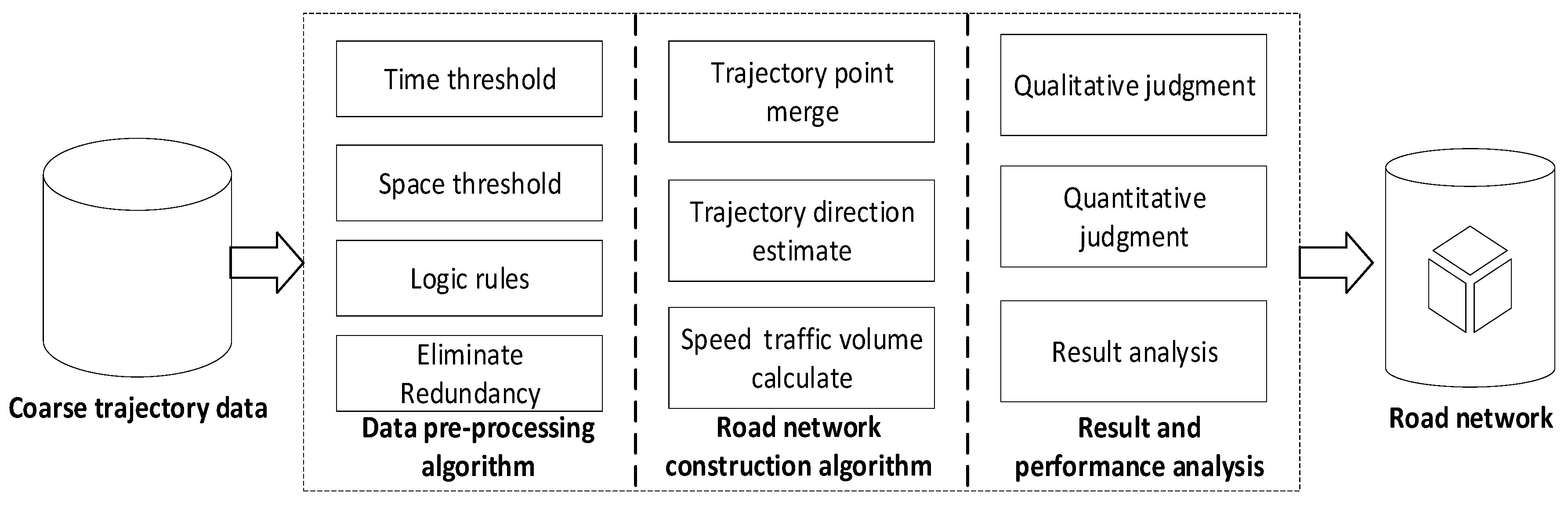
Our method contains a trajectory data preprocessing algorithm and a road network construction algorithm. The trajectory data preprocessing algorithm filters raw, noisy GPS data and organizes them into a set of trips; the road network construction algorithm builds a road network from scratch and calculates the corresponding average road traffic volume and speed. In detail, the data preprocessing algorithm processes the data by setting appropriate time, space, and logic thresholds by considering the positions and logical errors in the trajectory data from taxis during daily travel. In addition, the redundancy of the data is eliminated using logical rules. The road network construction algorithm assumes the initial road network is an empty graph. Then, the candidate trips are traversed to determine whether they should be inserted into the road network. Furthermore, the heading, average speed, and traffic volume of the constructed road network are calculated. We used the method to build a road network and then overlaid the resulting map onto an OpenStreetMap (OSM) data to qualitatively evaluate the degree of matching. For the quantitative evaluation, the F-score was calculated and compared with those of existing methods. An overview of our work is shown in Figure 1.
3.1. Data Preprocessing Algorithm
Vehicle trajectory data are sequences of a vehicle’s position and status information recorded continuously during travel. This information generally includes the vehicle’s ID, longitude, latitude, time, traveling speed, and travel direction. Formally, the trajectory data are expressed as (vehicle ID, time, longitude, latitude, travel speed, travel direction). Usually, the recording frequency of the data is set by the positioning equipment manufacturer and ranges from a few seconds to several minutes. The raw trajectory data based on the vehicle’s identification are recorded in chronological order and are not organized into sets of trips. Furthermore, there are many quality problems with the data; therefore, they are not suitable for directly constructing maps. The quality problems are as follows: (1) If the GPS receiver is turned off at one place and turned on at another place—for example, if the positioning device is broken—the direct connection between the two points does not reflect the actual path that the vehicle traveled. (2) The location accuracy is usually approximately several meters to 30 m. However, in areas such as high-rise buildings, shaded areas, tunnels, and overpasses, the positioning accuracy will be greatly affected, which will result in outlier positioning data. (3) There are long-term location-invariant points, which are not helpful for extracting road geometry information, and these extra points will increase the required calculation. (4) Other errors may exist in the data.
To better extract the road geometry information and improve the data quality, the path location information should be processed. Based on practical experience and assessments of the trajectory data, we assume that a reasonable trip or trajectory should meet the following characteristics: (1) The time interval of two consecutive points in a trajectory should be equal to the sampling interval; the sampling time is 90 s for our data. (2) The distance between two consecutive points is bounded. For our experimental data, it should be less than 1980 m because the speed of a vehicle on a road must be less than 80 km/h according to the local traffic regulations. (3) The maximum distance between any two points in a trajectory should be greater than a distance threshold. (4) When the vehicle speed is slow, there will be many trajectories within a short distance. (5) A trip must contain a certain number of locations, which depends on how long the vehicle travels. Therefore, we set the following rules for preprocessing:
- (1)
- If the time interval between two consecutive positioning measurements is Δt ≥ 600 s, then the trip is split into different trips. We chose 600 s as our threshold value because we found in analyzing all the time intervals between any two continuous position records in our experimental data that 93.97% of the time intervals are shorter than 90 s, 4.26% are longer than 600 s, and 2.04% are between 90 s and 600 s. A vehicle can travel a long distance in intervals that are longer than 600 s when the vehicle runs at a high speed, which can result in noise if we directly connect the initial and final positions for the time interval. We chose 600 s as the threshold to eliminate the 4.26% of edges that might be long-distance edges.
- (2)
- If the distance between two locations is Δd1 ≥ 2000 m, the trajectory is split into different trips. For our experimental data, the sampling interval of the experimental trajectory data is 90 s. We chose 2000 m as our threshold value because the maximum length between two consecutive points is 1980 m by precise calculation, as described above, and we loosen slightly the threshold.
- (3)
- If the maximum value of the distance between any two nodes in a trip is Δd2 < 200 m, the trip is deleted. We chose 200 m as our threshold value because we found that some trips in the experimental data involve roaming around small areas and the radii of these areas are less than 200 m. These areas may be informal car parks or gas stations. These trips do not contribute to the construction of the road network, but we can use them to extract POIs along the road in future work.
- (4)
- If two consecutive points are in the same position (here, if the distance between two points Δd3 < 5 m, we regard their locations as the same), only the first point in the trip is kept. In this way, we can eliminate data redundancy.
- (5)
- If the number of points in a trip, which is denoted by L, is less than 50, then the trip is deleted. In this way, we can eliminate certain invalid trips and speed up the processing. We chose 50 as the threshold because only 18% of all trips have greater than 50 points, but these contain approximately 80% of all positioning points.
After the above processing step, we can eliminate many errors and obtain the standard trip data. A pseudocode of the algorithm is shown in Algorithm 1.
| Algorithm 1 Preprocessing raw trajectory data |
| Input: Raw GPS trajectory data set C |
| Output: Cleaned trajectory dataset T |
| T = ∅; |
| For each point in C do |
| Trip = null; |
| If distance interval between point and its previous point Δd1 < 5 m, then |
| Continue; |
| End if |
| If time interval between point and its previous point Δt ≥ 600 s or Δt < 0 s or Δd1 ≥ 2000 m, then |
| If length of the trip L < 50 then |
| Trip = null; |
| Continue; |
| End if |
| If maximum distance between any two points in a Trip Δd2 < 200 m, then |
| Trip = null; |
| Continue; |
| End if |
| Add Trip to T; |
| End if |
| Add point to Trip |
| End For |
3.2. Road Network Construction Algorithm
The main steps of the algorithm are as follows: initialize the digital road network map as an empty graph; traverse the location points of all trajectories; insert the trip points into the graph or merge them with the existing graph points; update the graph line segment direction, speed, and traffic volume attributes; and convert the final graph into a road network map. The pseudocode of the algorithm is shown in Algorithm 2; details will be described below.
| Algorithm 2 Road network construction from dataset of trips |
| Input: Dataset T after preprocessing of raw trajectory data |
| Output: Directed graph G representing road network |
| G = ∅; |
| For each trip t in T do |
| prevNode = null; |
| For each node n in trips t do |
| If n should be merged with the existing edge e G, then |
| If n is near the complex road network then |
| Split_threshold d = intersection_threshold |
| Else: |
| Split_threshold d = normal_threshold |
| End if |
| If short_projection_distance > d, then |
| Add n to G, split the segment e by n, add the corresponding split_segment |
| edges (i.e., in_node of e → n and n → out_node of e) to G |
| Else: |
| merge n with nearest graph node v G |
| update the location of node v by considering the effect of n |
| End if |
| If prevNode ≠ null and there is no path in G from prevNode to n within less than 5 |
| hops, then |
| Add edge(prevNode → n) to G |
| prevNode = n; |
| End if |
| Else |
| Add node n to G; |
| If prevNode ≠ null, then |
| Add edge(prevNode → n) to G |
| prevNode = n; |
| End if |
| End for |
| End for |
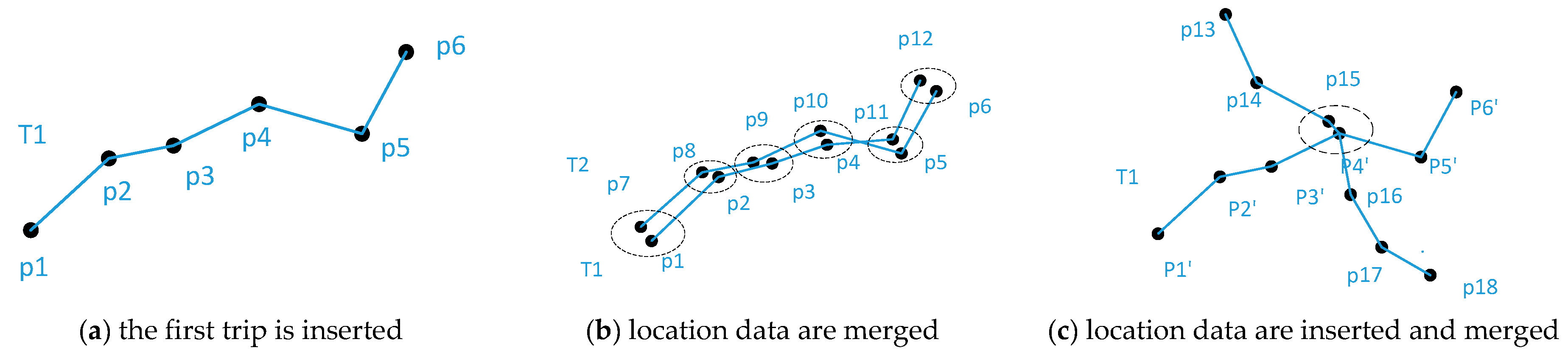
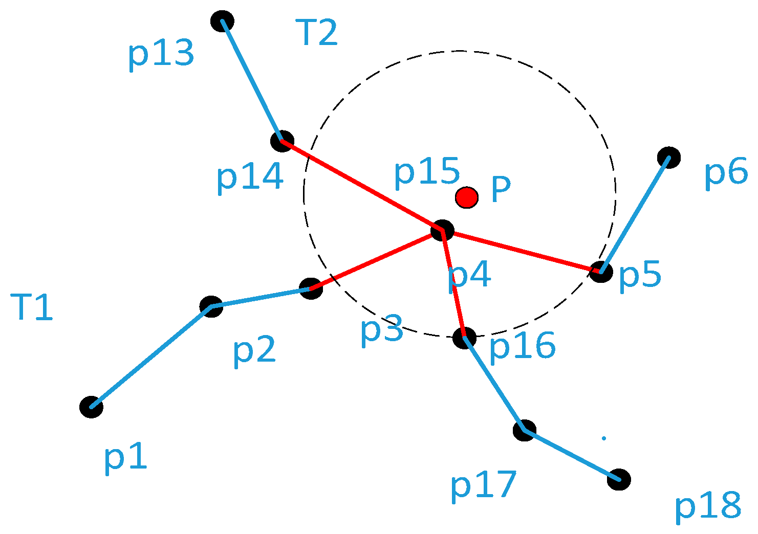
The process of Algorithm 2 is illustrated in Figure 2. The initial road network is empty. In Figure 2a, the first trip T1 is inserted into the empty map and every point in the trip is retained. In Figure 2b, the subsequent trip T2 is inserted into the map. The node of trip T2 is merged with the node of T1 because they are near enough to each other, which indicates that they are traveling on the same road. The points in the dotted circle are clustered to calculate a new location that represents all of the merged points. Figure 2c shows a circumstance in which not all nodes of a trip T3 need to be merged into the existing road network. Node p15 of T3 is merged with node p4’ of the newly calculated trip because they are close enough to each other; the other nodes of T3 will be inserted into the map because there are no existing nodes near enough to them. The method for determining how a trip should be merged with the existing edges is described in detail in the following.
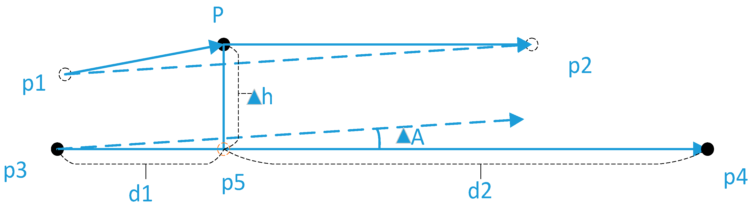
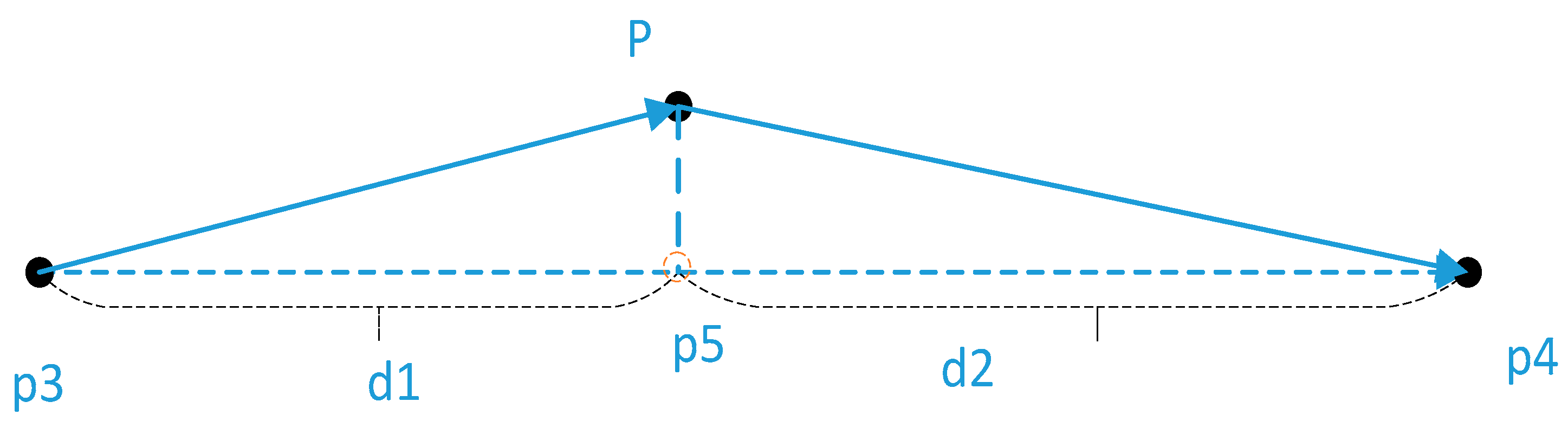
Merging method: Let P be the point to be merged. Find the graph edges within the merging threshold; a good spatial index can be used to speed up the process. For our experiment, we set the merge threshold to 50 m since the positioning accuracy of the data is approximately 30 m, and Rtree is used to find the candidate edges. Then, project P onto a candidate edge and determine, one by one, whether the following conditions are satisfied: (1) the projected point is on the projected line; (2) the projection distance is less than the merging threshold value (for example, 30 m); and (3) the direction of the point (which is represented by the direction from the point before it to the point after it; if one of these points is null, the direction is represented by the direction from the point before it to itself or from itself to the point after it) and the direction of the candidate edge are the same (the angle between them is less than a threshold). Here, we set 45 degrees as the threshold in our experiment since most of the road intersections are 90-degree intersections. When all of the above conditions are satisfied, the point P will be merged into the candidate edge. If the shortest length between the projected point and the two endpoints of the candidate edge is less than the split distance, the considered point is merged with the endpoint of the candidate edge that is closer to the projected point. When the merging process is carried out, the position of the endpoint is recalculated by weighted averaging of the merged points’ positions. For example, in Figure 3, whether point P should be merged into an existing edge needs to be determined. Points p1 and p2 are the locations before and after P, respectively. Here, the direction of line p1p2 is regarded as the direction of point P, the candidate edge is line p3p4, the projected point is p5, the projection distance is Δh, and two segments between the projected point and the two endpoints of the candidate edge are d1 and d2, respectively. If projected point p5 is on the candidate edge, the projection distance Δh is less than the threshold value of 50 m, and the angle ΔA is less than the threshold value of 45 degrees, then p3p4 satisfies the merging conditions. If d1 < d2 and d1 is smaller than the splitting threshold, point P is merged into p3 and the position of p3 is updated with the weighted average of the positions of P and p3, where the weight is determined by the traffic volume of the road. If d1 is greater than the split threshold, then edge p3p4 is split at point P. As shown in Figure 4, if d1 is greater than the splitting threshold, P is added to the graph node, edges p3P and Pp4 are added, and edge p3p4 is deleted.
It is worth emphasizing that the value of the splitting threshold is not fixed. Complex road networks (compared to straight roads or simple roads) such as traffic junctions, overpasses, and road intersections should be described in more detail in practice. Thus, a smaller splitting threshold value can be helpful. The key issue is determining how to judge whether the candidate edge belongs to a complex road network. This paper presents a method for judging whether a candidate edge is near the complex road network, by considering the directions of the roads around it.
Complex road network judgment method: If the average angle between the candidate edge and the edges that are within 100 m is greater than 45 degrees, the candidate edge is deemed to belong to the complex road network, and the splitting threshold value is set to 30 m. Otherwise, the candidate edge is deemed to be near a simple road and the splitting threshold is set to 5 km. For example, in Figure 5, P is the point to be judged. We first identify the edges that are within 100 m of P: namely, edges p3p4, p4p5, p14p15, and p15p16. Then, we calculate the average angle between p4p5 and the other edges. The average angle can be determined by calculating the absolute value of the cosine of each angle , where is the average angle, is the angle between the candidate edge and the edges that surround it, and n is the number of surrounding edges. For example, in Figure 4, P is the point to be judged; the candidate edge is p4p5, and the surrounding edges that are within 100 m are p14p15, p15p16, and p3p4. The average value of the cosines of the angles can be calculated via Equation (1):
If , we classify P as belonging to a complex road network.
4. Results of the Case Study of Beijing, China
Based on the algorithms described above, the method prototype was implemented in PythonTM programming language version 2.7.13, and an experiment was carried out on a server with Intel Xeon CPU [email protected] GHz and 64 GB memory. Both qualitative and quantitative evaluations were performed. For the qualitative evaluation, the results were overlaid onto an OpenStreetMap tile map. For the quantitative evaluation, the F-score [30] was used and compared with those of Cao and Krumm’s method [23] and Davies et al.’s method [20], both of which are classical methods. The experimental data and results are described in the following.
4.1. Introduction of GPS Trajectory Data and Ground-Truth Map
The experimental GPS trajectory data came from 200 taxis that had been equipped with GPS devices for approximately one month of daily travel in Beijing. The main area of Beijing is approximately 2243 km2. The experimental area covers approximately 75% of the urban vehicle roads. The location sampling interval is 90 s, and the positioning accuracy of those data is several meters to approximately 30 m. The total number of positioning data is approximately 5.76 million. Example GPS trajectory data are shown in Table 2, which includes the following fields: vehicle ID, which uniquely identifies a vehicle; time; longitude; latitude; speed (m/s); and direction (degree), which is relative to north. We chose OpenStreetMap as our ground-truth map, which expresses freeways and arterial roads in detail and can be downloaded freely.
4.2. Experiment Results and Discussion
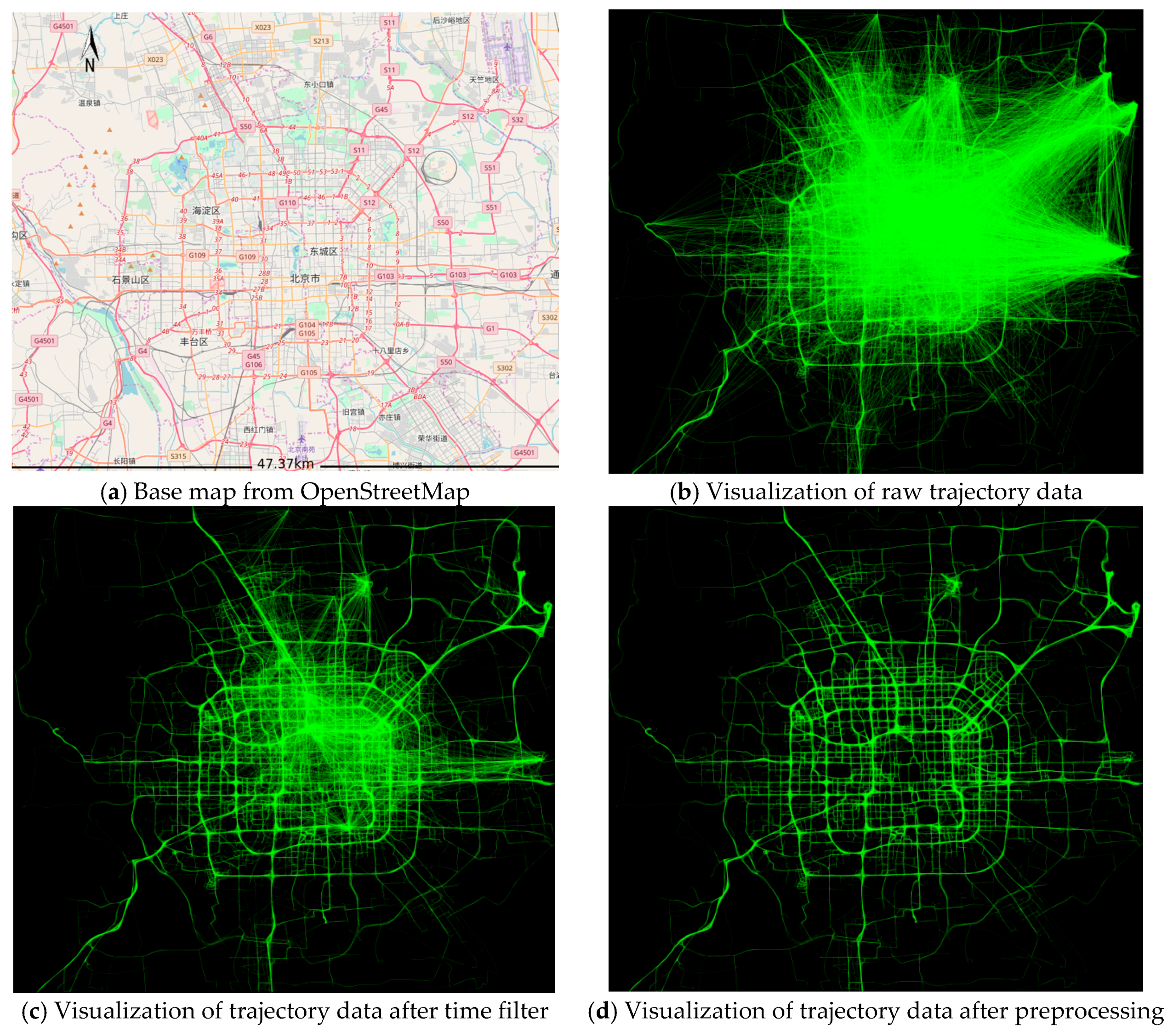
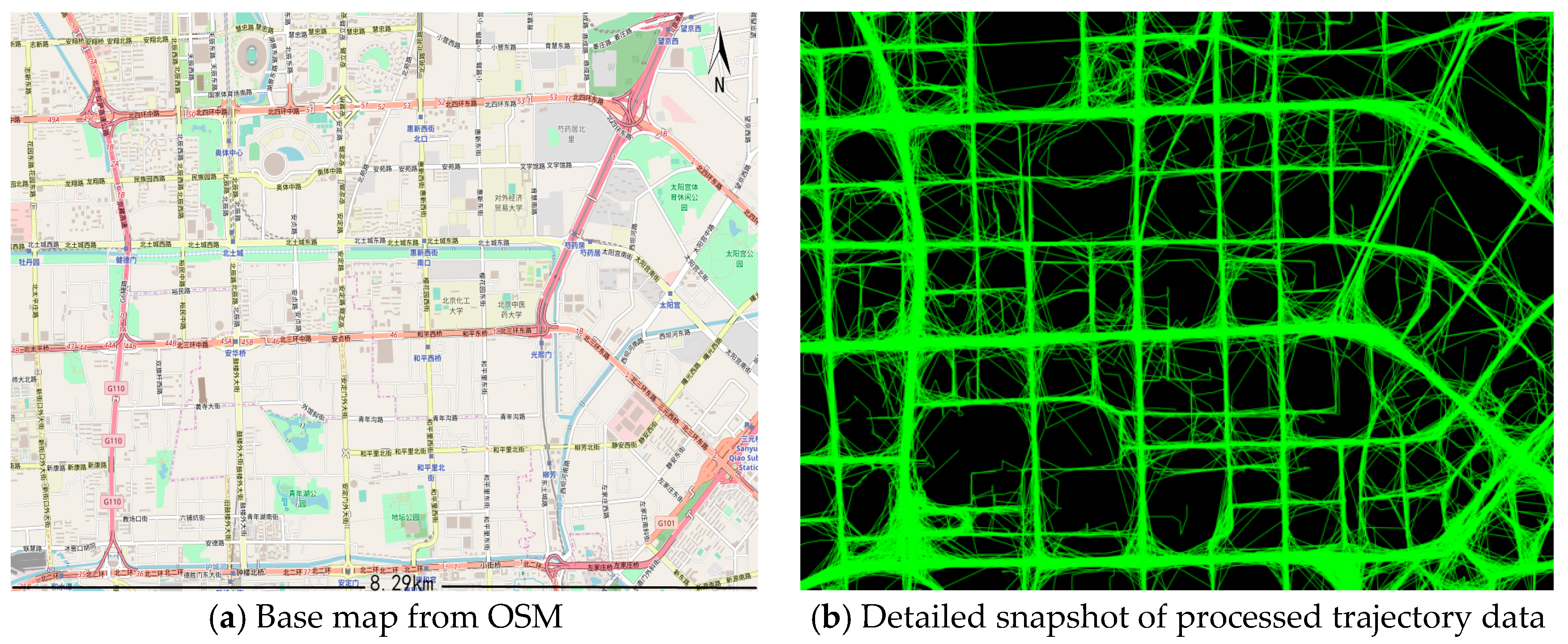
It took 2 h 47 min 9 s to finish the experiment. Figure 6 shows an overview of the results of the data preprocessing algorithm. Figure 6a is the base map of the study area from OSM, which covers most of the road network of Beijing. In Figure 6b, we connected the locations along the trajectory in accordance with their chronological order. The skeleton of the road network can be built, but it is covered by many cluttered and illegible trajectories. After preprocessing, the trajectory data better reflects the skeleton of urban roads. As shown in Figure 6c, the trajectory data were filtered by using time thresholds 0 s < Δt < 600 s. Figure 6d is the final result of the entire preprocessing step, in which 1.27 million positioning data were deleted and the remaining 4.49 million positioning data were organized into 12,364 trips. The final generated networks reflect the most important connectivity and geometric properties of the real road network, as shown in Figure 6d. Based on an in-depth consideration of the processed trajectories (see Figure 7), there are too many trips on the same road, they do not completely overlap with one another, and the road’s heading and traffic volume are not clear. In addition, there are many messy lines near the intersection. Those problems will be addressed later by the road network construction algorithm.
With an increase in Δt, the number of non-conforming trips increases. With a decrease in Δt, each trip contains fewer location points and the number of trips increases. With a decrease in Δd1, the length of the line segments included in each trip decreases and the data volume of the trip increases. As L decreases, the number of points in each trip increases and the number of trips that meet the requirement increases. With an increase in Δd2, there is a chance that invalid trips will be generated. With an increase in Δd3, more data can be deleted but the resulting trips will not appear smooth.
By preprocessing the trajectory data, we obtain a set of relatively smooth trips that, although rough, describe the connectivity and geometric properties of the road network very well. Through the road network construction algorithm, we obtain a road network map that is expressed as a graph. In addition to the connectivity and geometric properties of the road network, the heading and traffic volume of the road network can be calculated. Some properties of the generated road network are listed in Table 3.
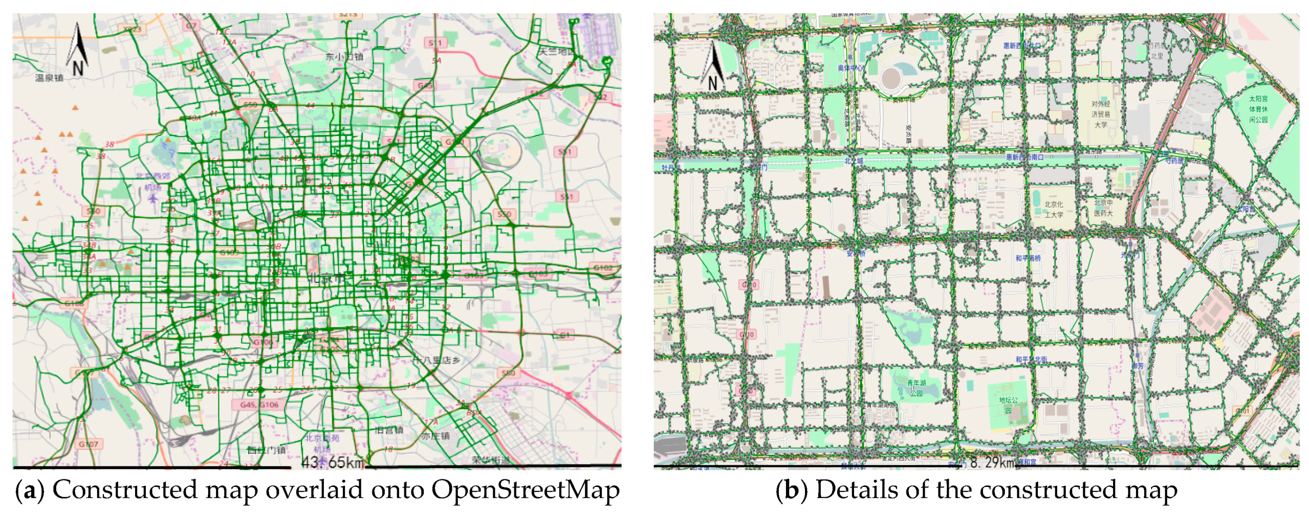
Figure 8 shows the results of the constructed road network. The constructed road network, which is represented by green lines, was overlaid onto the OSM. Figure 8a shows an overview of the matching generated roads and Figure 8b shows the details of the generated roads. The geometric, connectivity, and heading properties of the road network are well matched overall with those of the OSM base map, which shows that our method can effectively generate a road network.
Liu et al. [21] use the F-score to quantitatively measure the performance of a method inspired by information retrieval evaluation. In their method, they first calculate the precision and recall of each inferred road where and , in which denotes the length of the road, M is the extracted map, Ground is the ground-truth map, and denotes the matched parts. Then, . We used their method to quantitatively evaluate our method and compared it to Cao and Krumm’s [23] and Davies et al.’s [20] methods. Figure 9 shows the F-scores of our method compared to those of the two existing methods. As shown in the figure, our method obtains a higher F-score than the other methods.
From the experimental results above, we conclude that our method can generate a road network successfully and effectively. However, there are still five major defects in the experimental result:
- (1)
- Certain roads appear on the reference base map but not on the constructed map. This discrepancy occurs because the degree of overlay of the GPS trajectory data is limited, which means the experimental trajectory cannot reflect all the roads, especially certain footways through which vehicles cannot pass. Moreover, the experimental data are old; therefore, the constructed map does not reflect newly constructed roads.
- (2)
- The constructed map is more “dentate” than the reference base map because the density of points in the constructed road is too high. The density can be reduced by using a high splitting threshold value, although this shortcoming cannot be completely eliminated. A future research topic could be the further smoothing of the line segments.
- (3)
- The constructed map recognizes the overpass as an intersection because we model the road network as a planar graph. The precise extraction of information about complicated road networks, such as overpasses and intersections, could be further studied in the future.
- (4)
- There are many messy edges near complex roads, which do not reflect the intersections’ actual situations. It is difficult to extract a directly usable road network using an automatic method because of the inherent positioning error of GPS and the complexity of the roads. In the future, we may try to determine the rough shape of the intersection or train certain intersection models to alleviate the problem.
- (5)
- In some instances, adjacent intersections have merged into one because those roads are too close to each other. The problem can be addressed by adjusting the parameters of the projection distance Δh.
Most of the threshold values for the algorithms discussed above were determined by estimations based on our experimental data, and a few of them were selected based on experience. Therefore, basic estimates based on the data of the position data sampling time, data location accuracy, and average running speed should be obtained to determine the threshold values and make the result more accurate. To assess the method proposed in this paper, we performed a qualitative evaluation by overlaying the constructed road network onto the OSM and performed a quantitative evaluation based on the F-score. Neither method is perfect for evaluating the overall quality (in all aspects) of the constructed map. However, the results reflect certain properties of the real road network. In our future work, different measurement methods such as Hausdorff distance and Fréchet distance will be considered for evaluating the geometric and topological properties of road networks. In the future, using the trajectory data of public and private vehicles, substantial amounts of road mapping information—including geometric information of the road, POIs, traffic regulations, and traffic conditions—will be detected, identified, and extracted in real time and then automatically transformed into digital road maps, making this field more important and attractive.
5. Conclusions and Future Work
Accurate digital road maps are of great importance for efficient travel. Old methods of collecting and updating road mapping information are usually slow and expensive. Ubiquitous vehicle GPS devices generate massive amounts of trajectory data, which provide an unprecedented opportunity to automatically generate navigational digital maps in real time. The main contribution of this paper is a new method for extracting road information from the daily travel trajectory data of ordinary vehicles, which includes a constraint rule-based data preprocessing algorithm and a road network construction algorithm. Through the preprocessing of trajectory data, noise data are eliminated and then the road geometry information is extracted using the road network construction algorithm. In the road network construction algorithm, when determining the splitting threshold values, the complexity of the road network is considered by utilizing a complex road detection method. This method can complement the traditional field surveying method and remote sensing image extraction method. Additionally, the heading, speed, and traffic volume along each road are calculated and recorded. Finally, the road network can be obtained. The experimental results demonstrate the effectiveness of our proposed method.
Constructing digital maps from vehicle trajectory data is a promising area for the near future because it can provide an abundance of real-time information. Such maps can contain the geometrical positions of roads, the topological relation between roads, the traveling speeds, and so forth. Therefore, they can be utilized in many applications, such as in automatic driving. In future research, we will attempt to extract additional navigational information such as parking lots and gas stations, and improve the accuracy of the network in complex areas such as road intersection areas, overpasses, and tunnels. In view of the complexity of our road network construction algorithm, we will rebuild it in Apache SparkTM to help accelerate this process in the future. Then, the real-time construction of road networks can be expected.
Acknowledgments
This paper was funded by the National Key Research and Development Program under grant No. 2016YFC0803108, the Public Welfare Industry Research Special Fund Program under grant No.201512032, the National Natural Science Foundation of China under grant No. 41701461, and the Basic Scientific Research Fund Project of Chinese Academy of Surveying and Mapping under grant No. 7771614. We express our thanks to the anonymous reviewer for constructive comments.
Author Contributions
Yongchuan Zhang and Jiping Liu were responsible for the research design and experiments. Xinlin Qian led the writing of the paper, with Fuhao Zhang and Agen Qiu contributing materials.
Conflicts of Interest
The authors declare no conflict of interest. The founding sponsors had no role in the design of the study, nor in the collection, analyses, or interpretation of data, nor in the writing of the manuscript or the decision to publish the results.
References
- El-Sheimy, N.; Schwarz, K.P. Navigating urban areas by VISAT—A mobile mapping system integrating GPS/INS/digital cameras for GIS applications. Navigation 1998, 45, 275–285. [Google Scholar] [CrossRef]
- Sghaier, M.O.; Lepage, R. Road Extraction From Very High Resolution Remote Sensing Optical Images Based on Texture Analysis and Beamlet Transform. IEEE J. Sel. Top. Appl. Earth Obs. Remote Sens. 2016, 9, 1946–1958. [Google Scholar] [CrossRef]
- Yuan, J.; Cheriyadat, A.M. Image driven GPS trace analysis for road map inference. In Proceedings of the 21st ACM SIGSPATIAL International Conference on Advances in Geographic Information Systems, Orlando, FL, USA, 5–8 November 2013; pp. 480–483. [Google Scholar]
- Goodchild, M.F. Citizens as sensors: The world of volunteered geography. GeoJournal 2007, 69, 211–221. [Google Scholar] [CrossRef]
- Li, H.; Kulik, L.; Ramamohanarao, K. Automatic Generation and Validation of Road Maps from GPS Trajectory Data Sets. In Proceedings of the 25th ACM International on Conference on Information and Knowledge Management, Indianapolis, IN, USA, 24–28 October 2016; pp. 1523–1532. [Google Scholar]
- Qiu, J.; Wang, R. Road Map Inference: A Segmentation and Grouping Framework. ISPRS Int. J. Geo-Inf. 2016, 5, 130. [Google Scholar] [CrossRef]
- Zhou, Y.; Zhang, Y.; Ge, Y.; Xue, Z.; Fu, Y.; Guo, D.; Shao, J.; Zhu, T.; Wang, X.; Li, J. An efficient data processing framework for mining the massive trajectory of moving objects. Comput. Environ. Urban Syst. 2015, 61, 129–140. [Google Scholar] [CrossRef]
- Jiang, S.; Fiore, G.A.; Yang, Y.; Ferreira, J., Jr.; Frazzoli, E.; González, M.C. A review of urban computing for mobile phone traces: Current methods, challenges and opportunities. In Proceedings of the 2nd ACM SIGKDD International Workshop on Urban Computing, Chicago, IL, USA, 11 August 2013; p. 2. [Google Scholar]
- Woodard, D.; Nogin, G.; Koch, P.; Racz, D.; Goldszmidt, M.; Horvitz, E. Predicting travel time reliability using mobile phone GPS data. Transp. Res. Part C Emerg. Technol. 2017, 75, 30–44. [Google Scholar] [CrossRef]
- Kuntzsch, C.; Sester, M.; Brenner, C. Generative models for road network reconstruction. Int. J. Geogr. Inf. Sci. 2016, 30, 1012–1039. [Google Scholar] [CrossRef]
- Fang, W.; Hu, R.; Xu, X.; Xia, Y.; Hung, M.-H. A novel road network change detection algorithm based on floating car tracking data. Telecommun. Syst. 2016, 1–7. [Google Scholar] [CrossRef]
- Gonzalez, M.C.; Hidalgo, C.A.; Barabasi, A.-L. Understanding individual human mobility patterns. Nature 2008, 453, 779–782. [Google Scholar] [CrossRef] [PubMed]
- Kong, X.; Xu, Z.; Shen, G.; Wang, J.; Yang, Q.; Zhang, B. Urban traffic congestion estimation and prediction based on floating car trajectory data. Future Gener. Comput. Syst. 2016, 61, 97–107. [Google Scholar] [CrossRef]
- Tang, L.; Yang, X.; Kan, Z.; Li, Q. Lane-Level Road Information Mining from Vehicle GPS Trajectories Based on Naïve Bayesian Classification. ISPRS Int. J. Geo-Inf. 2015, 4, 2660–2680. [Google Scholar] [CrossRef]
- Zhou, Y.; Fang, Z.; Thill, J.-C.; Li, Q.; Li, Y. Functionally critical locations in an urban transportation network: Identification and space–time analysis using taxi trajectories. Comput. Environ. Urban Syst. 2015, 52, 34–47. [Google Scholar] [CrossRef]
- Li, H.; Kulik, L.; Ramamohanarao, K. Robust inferences of travel paths from GPS trajectories. Int. J. Geogr. Inf. Sci. 2015, 29, 2194–2222. [Google Scholar] [CrossRef]
- Qiu, J.; Wang, R. Inferring road maps from sparsely sampled GPS traces. J. Locat. Based Serv. 2016, 10, 111–124. [Google Scholar] [CrossRef]
- Ahmed, M.; Karagiorgou, S.; Pfoser, D.; Wenk, C. A comparison and evaluation of map construction algorithms using vehicle tracking data. GeoInformatica 2015, 19, 601–632. [Google Scholar] [CrossRef]
- Biagioni, J.; Eriksson, J. Map inference in the face of noise and disparity. In Proceedings of the 20th International Conference on Advances in Geographic Information Systems, Redondo Beach, CA, USA, 6–9 November 2012; pp. 79–88. [Google Scholar]
- Davics, J.; Beresford, A.R.; Hopper, A. Scalable, distributed, real-time map generation. IEEE Pervasive Comput. 2006, 5, 47–54. [Google Scholar]
- Liu, X.; Biagioni, J.; Eriksson, J.; Wang, Y.; Forman, G.; Zhu, Y. Mining large-scale, sparse GPS traces for map inference: Comparison of approaches. In Proceedings of the 18th ACM SIGKDD International Conference on Knowledge Discovery and Data Mining, Beijing, China, 12–16 August 2012; pp. 669–677. [Google Scholar]
- Ahmed, M.; Wenk, C. Constructing street networks from GPS trajectories. In Algorithms–ESA 2012; Springer: Berlin/Heidelberg, Germany, 2012; pp. 60–71. [Google Scholar]
- Cao, L.; Krumm, J. From GPS traces to a routable road map. In Proceedings of the 17th ACM SIGSPATIAL International Conference on Advances in Geographic Information Systems, Seattle, WA, USA, 4–6 November 2009; pp. 3–12. [Google Scholar]
- Ekpenyong, F.; Palmer-Brown, D.; Brimicombe, A. Extracting road information from recorded GPS data using snap-drift neural network. Neurocomputing 2009, 73, 24–36. [Google Scholar] [CrossRef]
- Niehöfer, B.; Burda, R.; Wietfeld, C.; Bauer, F.; Lueert, O. GPS community map generation for enhanced routing methods based on trace-collection by mobile phones. In Proceedings of the First International Conference on Advances in Satellite and Space Communications SPACOMM 2009, Colmar, France, 20–25 July 2009; pp. 156–161. [Google Scholar]
- Rogers, S.; Langley, P.; Wilson, C. Mining GPS data to augment road models. In Proceedings of the Fifth ACM SIGKDD International Conference on Knowledge Discovery and Data Mining, San Diego, CA, USA, 15–18 August 1999; pp. 104–113. [Google Scholar]
- Xie, X.; Liao, W.; Aghajan, H.; Veelaert, P.; Philips, W. Detecting Road Intersections from GPS Traces Using Longest Common Subsequence Algorithm. ISPRS Int. J. Geo-Inf. 2016, 6, 1. [Google Scholar] [CrossRef]
- Karagiorgou, S.; Pfoser, D. On vehicle tracking data-based road network generation. In Proceedings of the 20th International Conference on Advances in Geographic Information Systems, Redondo Beach, CA, USA, 6–9 November 2012; pp. 89–98. [Google Scholar]
- Fathi, A.; Krumm, J. Detecting road intersections from GPS traces. In Geographic Information Science; Springer: Berlin/Heidelberg, Germany, 2010; pp. 56–69. [Google Scholar]
- Biagioni, J.; Eriksson, J. Inferring Road Maps from Global Positioning System Traces Survey and Comparative Evaluation. Transp. Res. Rec. 2012, 2291, 61–71. [Google Scholar] [CrossRef]
- Edelkamp, S.; Schrodl, S. Route planning and map inference with global positioning traces. Comput. Sci. Perspect. 2003, 2598, 128–151. [Google Scholar]
- Zhang, L.; Thiemann, F.; Sester, M. Integration of GPS traces with road map. In Proceedings of the Second International Workshop on Computational Transportation Science, San Jose, CA, USA, 2 November 2010; pp. 17–22. [Google Scholar]
Figure 1.
The framework of the map auto-construction method. First, a constraint rule-based trajectory data preprocessing algorithm is used to remove noise, which includes a time threshold, space threshold, logic threshold, and redundancy elimination. Second, a road network construction algorithm is used to generate a digital map using processes of trajectory point clustering, trajectory direction estimation, and average speed calculation. Third, the performance of the method is examined by comparing the constructed map with the OpenStreetMap and calculating the F-score for comparison with typical existing methods.

Figure 2.
Road network construction process diagram. (a) The first trip is inserted, (b) the second trajectory is inserted and integrated with existing nodes, and (c) the third trip is inserted and the merging method is used according to the position of the point that is being inserted.
Figure 2.
Road network construction process diagram. (a) The first trip is inserted, (b) the second trajectory is inserted and integrated with existing nodes, and (c) the third trip is inserted and the merging method is used according to the position of the point that is being inserted.

Figure 3.
Schematic of merging a point into an existing road network.

Figure 4.
Schematic for splitting a candidate edge into two more detailed edges.

Figure 5.
Schematic for determining a complex road network.

Figure 6.
Base map and snapshots for the preprocessing trajectory data from Beijing. (a) A base map from OpenStreetMap. (b) A visualization of 5.76 million raw trajectory data points using OpenCV. (c) A visualization of those trajectory data after time filter 0 s < Δt < 600 s. (d) A visualization of the trajectory data after preprocessing. As shown in the picture, our preprocessing algorithm can effectually remove noise.

Figure 7.
A detailed look at the processed trajectories. (a) A subarea of the base map from OSM, and (b) a snapshot of the processed trajectory. As shown in (b), there are many messy lines around road intersections, which require further processing to extract the real roads.
Figure 7.
A detailed look at the processed trajectories. (a) A subarea of the base map from OSM, and (b) a snapshot of the processed trajectory. As shown in (b), there are many messy lines around road intersections, which require further processing to extract the real roads.

Figure 8.
Comparison of the constructed road network with the ground truth. The result is overlaid onto OpenStreetMap, which shows that the resulting map matches the base map very well. (a) The overall scenario; the constructed road network is represented as a green graph. (b) One subset area of the constructed road network in detail; the directions of the roads are expressed using black arrows.

Figure 9.
Comparison of the F-scores of our method vs existing methods using different matching thresholds during geometry sampling.
Figure 9.
Comparison of the F-scores of our method vs existing methods using different matching thresholds during geometry sampling.


Table 1.
Algorithm categories.
| Algorithm Category | Representative Algorithms |
|---|---|
| Point clustering | Biagioni and Eriksson [19], Davies et al. [20], Edelkamp and Schrodl [31] |
| Incremental trace insertion | Cao and Krumm [23], Ahmed and Wenk [22], Rogers and Langley [26], Zhang and Thiemann [32] |
| Intersection linking | Karagiorgou and Pfoser [28], Fathi and Krumm [29] |
Table 2.
Example of the global positioning system (GPS) trajectory data.
| Vehicle ID | Time | Longitude | Latitude | Speed (m/s) | Direction (degree) |
|---|---|---|---|---|---|
| 756,945 | 2012–11–30 19:17:05 | 116.4433975 | 39.9258118 | 26.00 | 170 |
| … | … | … | … | … | … |
| 757,255 | 2012–11–30 19:23:05 | 116.4288635 | 39.9076500 | 2.00 | 208 |
| 757,255 | 2012–11–30 19:34:35 | 116.4233017 | 39.9000549 | 15.00 | 265 |
Table 3.
Statistics of the resulting digital map.
| Property | Value |
|---|---|
| Number of nodes | 109,324 |
| Number of road segments | 157,755 |
| Average length of a road segment | 1380.12 m |
| Average road speed | 8.32 km/h |
© 2017 by the authors. Licensee MDPI, Basel, Switzerland. This article is an open access article distributed under the terms and conditions of the Creative Commons Attribution (CC BY) license (http://creativecommons.org/licenses/by/4.0/).
Share and Cite
MDPI and ACS Style
Zhang, Y.; Liu, J.; Qian, X.; Qiu, A.; Zhang, F. An Automatic Road Network Construction Method Using Massive GPS Trajectory Data. ISPRS Int. J. Geo-Inf. 2017, 6, 400. https://0-doi-org.brum.beds.ac.uk/10.3390/ijgi6120400
AMA Style
Zhang Y, Liu J, Qian X, Qiu A, Zhang F. An Automatic Road Network Construction Method Using Massive GPS Trajectory Data. ISPRS International Journal of Geo-Information. 2017; 6(12):400. https://0-doi-org.brum.beds.ac.uk/10.3390/ijgi6120400
Chicago/Turabian StyleZhang, Yongchuan, Jiping Liu, Xinlin Qian, Agen Qiu, and Fuhao Zhang. 2017. "An Automatic Road Network Construction Method Using Massive GPS Trajectory Data" ISPRS International Journal of Geo-Information 6, no. 12: 400. https://0-doi-org.brum.beds.ac.uk/10.3390/ijgi6120400
Note that from the first issue of 2016, this journal uses article numbers instead of page numbers. See further details here.