1. Introduction
With the technical developments in location-aware technologies such as GPS (global positioning system), RFID (radio-frequency identification), WiFi and bluetooth, the position changes of moving objects over time can be tracked more easily than ever before. This has caused a proliferation of rich and voluminous movement data. Specific types of movement data include transportation-related movement data [
1,
2,
3,
4,
5], animal movement data [
6,
7,
8], eye movement data [
9], sports movement data [
10,
11,
12], as well as natural phenomena movement data [
13]. Benefiting from the large amount of tracked movement data, the analysis of movement data has become a state-of-the-art research theme in the community of geographical information science (GIScience). Currently, numerous methods to analyze movement data, such as movement pattern mining [
6,
14,
15], movement visualization [
16,
17,
18] and movement modelling [
19,
20,
21], have been undertaken extensively. In addition, the study of interactions in movement data has become active recently, but is still in its infancy [
22,
23]. In this paper, we mainly focus on exploring the interaction issues in movement data aiming to provide additional insights into this relatively new research topic.
Moving objects commonly move in geographical space, in which the geographical context (e.g., the environments where moving objects occur) is considered one of the important components. Therefore, the interactions in movement data can be categorized as the interactions between geographical contexts, the interactions between moving objects and geographical contexts, and the interactions between moving objects themselves. In this paper, we only consider the interactions between/among moving objects themselves. Interactions can be classified as static interactions or dynamic interactions [
24]. In spatio-temporal data (e.g., movement data), static interactions are purely described by spatial properties, without taking account of the possibility of temporal avoidance or attraction between individuals, while dynamic interactions are defined based on both spatial and temporal components [
25]. Hence, ‘dynamic interaction’ is sometimes synonymously termed as ‘spatio-temporal interaction’ [
22]. We mainly focus on dynamic interactions in this paper.
Generally, dynamic interactions can be defined as the way the movements of individuals are related or the inter-dependency in the movements of individuals. For example, attraction and avoidance are two typical kinds of dynamic interactions [
25]. Typical research on dynamic interactions in movement data within the domain of GIScience is listed as follows. Miller [
26] analyzed the dynamic interactions between individuals based on the GPS data of animals using five different techniques, thereby comparing the results acquired by the different techniques. Later, a null model approach [
25] was developed by the same author to compare six dynamic interaction metrics using data on five brown hyena dyads in Northern Botswana. The comparisons highlighted the need for further study of appropriate methods for measuring and interpreting dynamic interactions [
25]. Long et al. [
23] introduced a new method, dynamic interactions (termed DI), for measuring dynamic interactions between pairs of moving objects. Six simulated datasets and two applied examples (i.e., team sports and wildlife) were used to validate the DI method. The results showed that the DI method was able to be used to measure dynamic interactions in movement data. Long et al. [
27] executed an examination of eight currently available indices of dynamic interactions in wildlife telemetry studies and compared the effectiveness of the indices. Long [
22] examined the statistical properties of a suite of currently available methods in dynamic interactions. In this work, the ability of each method in characterizing and capturing different patterns of dynamic interactions was examined in practice. Konzack et al. [
28] proposed a new approach to analyze interactions between two trajectories and developed a prototype visual analytics tool to evaluate the approach based on three datasets.
By summarizing the aforementioned studies, we can find that the current research mainly focuses on either comparing or evaluating existing interaction methods based on various datasets, or developing new methods to measure dynamic interactions between a pair of trajectories. Besides, most of the current research on dynamic interactions has been done at a single temporal scale. Few work has focused on exploring the dynamic interactions among multiple moving objects and at multiple temporal scales. In addition, few have aimed at exploring the importance of each individual and identifying the individuals which play relatively important roles in maintaining specific types of interaction patterns. Hence, in order to achieve the above-mentioned explorations, we develop a hybrid approach combining the multi-temporal scale spatio-temporal network (MTSSTN) and the continuous triangular model (CTM). Currently, networks are widely used to explore many systems. However, in the data-rich era, it appears necessary to deal with data that are temporally evolving. To this end, temporal networks are proposed and applied to various domains [
29,
30,
31]. More recently, spatio-temporal networks have been proposed to enhance the abilities of networks [
32,
33]. In this paper, we propose a novel spatio-temporal network (i.e., multi-temporal scale spatio-temporal network) to extend the analytics applicability of spatio-temporal networks at multiple temporal scales. We then integrate the MTSSTN with the CTM to compose our proposed approach. In this approach, first, the relative trajectory calculus (RTC) [
34] is employed to derive specific types of interaction patterns. Second, the MTSSTN is generated based on a specific interaction pattern. Third, for each MTSSTN, the interaction intensity measures and three frequently used centrality measures (i.e., degree, betweenness and closeness) [
35,
36] in network theory are calculated. Finally, the results are visualized using a multi-temporal scale visualization tool, the CTM [
12,
37], and the results are analyzed based on the generated CTM diagrams. Based on the generated CTM diagrams, the following aims can be achieved for each interaction pattern at multiple temporal scales: (1) exploring the interaction intensities between any two individuals; (2) exploring the general interaction intensities among multiple individuals, and (3) exploring the importance of each individual and identifying the most important individuals by applying map algebra operations to multiple CTM diagrams.
The remainder of this paper is organized as follows.
Section 2 gives a brief introduction to network theory, RTC and CTM. In
Section 3, the methodology of the proposed approach is described in detail. In
Section 4, a case study of football is conducted using the proposed approach, and the results are analyzed. Some advantages and disadvantages of the proposed approach are discussed in
Section 5. Finally, in
Section 6, the conclusions and recommendations for future work are described.
2. Background Knowledge
In this section, the basic information on network theory, the relative trajectory calculus (RTC) and the continuous triangular model (CTM) are introduced, so that one can be able to understand the proposed approach easily.
2.1. Network Theory
A large number of systems, either natural or man-made, are structured in the form of networks. Therefore, network theory has been widely used to explore the complex systems existing in many domains. Typical examples include social networks, World Wide Web, transportation networks, academic cooperation networks, biological networks, and so forth [
35,
38]. Essentially, a network is a graph which can be represented as
, where
and
respectively denote the set of vertices and edges. A graph can be connected or disconnected, directed or undirected, and weighted or unweighted. A connected, undirected and unweighted graph with
n vertices can be represented by an adjacency matrix
as denoted by Equation (1):
Note that in this case, matrix is symmetric. Besides, all diagonal elements of are zero. Hence, in practice, we can just calculate either the top right or the bottom left part of in order to reduce the complexity. The other part of can be computed via a symmetric transformation.
Several measures have been proposed to characterize the topological structural properties of a network or to investigate the importance of vertices. Among these measures, centrality measures are widely used. Frequently used centrality measures are degree, betweenness and closeness. In a graph, the degree of a vertex corresponds to the number of vertices that are directly connected to this vertex. Formally, the degree of a given vertex
is calculated as follows:
where
represents the degree and
n is the total number of vertices in the graph.
The betweenness of a vertex measures to what extent the vertex is located in between the paths that connect pairs of vertices. Formally, the betweenness of a given vertex
is calculated as follows:
where
denotes the betweenness,
is the number of shortest paths from vertex
to vertex
that pass through vertex
,
represents the number of shortest paths from vertex
to vertex
, and
n is the total number of vertices in the graph.
The closeness of a vertex measures the closeness of a vertex to all other vertices in a graph. Formally, the closeness of a vertex
is calculated as follows:
where
denotes the closeness,
is the shortest path from vertex
to vertex
, and
n is the total number of vertices in the graph.
The measures of degree, betweenness and closeness describe the status of vertices. As degree only considers the relations between a vertex and its immediate neighboring vertices, it is characterized as a local measure. In contrast, betweenness and closeness are considered as global measures, since they take the relations of a vertex and all other vertices into account. Specific to the objects in the real world, if an object has a high degree value, it means that the object directly connects to a large number of other objects, hence, it is a relatively important object. Betweenness evaluates to what extent a given object is part of the shortest paths that connect to any two other objects. A high betweenness value indicates that the object plays an important role in the connectivity of other objects as a ‘bridge’, hence, without this object, the connectivity of other objects might be broken. Closeness reflects how far (on average) an object is to every other object. This gives a sense to what extent an object is integrated or segregated with respect to other objects. A high closeness value denotes that the object is more integrated to all other objects, thus is more central and important.
2.2. Relative Trajectory Calculus (RTC)
The Relative Trajectory Calculus (RTC) was proposed by Van de Weghe [
34] as a qualitative approach to represent the spatio-temporal relationships between two disjoint moving objects based on describing their relative trajectories. Important in this calculus is that an object moving during a time interval
I, which starts at time stamp
t1 and ends at time stamp
t2, is represented by means of a vector starting at
t1 and ending at
t2. Two objects moving during the same time interval can be represented by two vectors, each corresponding to a specific object. Using a single character label to denote the distance relation between the two objects, the RTC relationship between the two objects is determined. In the following, the RTC relationship is introduced in detail.
Assume: moving objects k and l, and time stamp t
k|t denotes the position of k at t
l|t denotes the position of l at t
d(u, v) denotes the Euclidean distance between two positions u and v
t1 t2 denotes that t1 is temporally before t2
: the distance between
k and
l decreases:
: the distance between
k and
l remains the same:
: the distance between
k and
l increases:
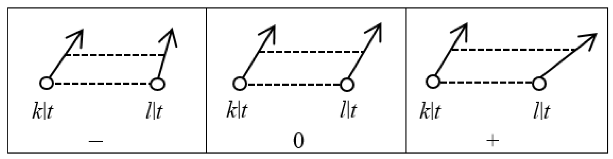
According to the relationship syntax between two moving objects, three RTC relations can be distinguished, as illustrated in
Figure 1. For example, the RTC relation ‘−’ indicates that the distance between the two objects before
t is larger than the distance between the two objects after
t. As the relations can represent the inter-relationship between two moving objects, they can be adopted to denote specific types of interaction patterns. Hence, three types of interaction patterns (i.e., attraction pattern, stability pattern and avoidance pattern) can be derived based on the RTC relations. The relationship between the RTC relations and the three types of interaction patterns is shown in
Table 1.
2.3. Continuous Triangular Model (CTM)
The continuous triangular model (CTM) is an extension of the triangular model (TM), a 2D representation of time intervals that was initially introduced by Kulpa [
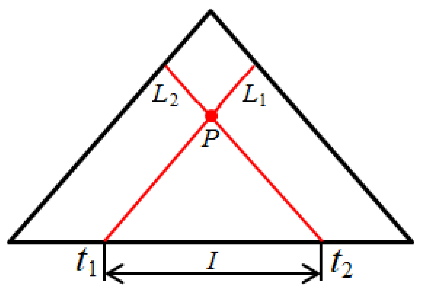
39]. In the TM, any time interval is represented by a corresponding point. For example, in
Figure 2, the time interval
I, which starts at
t1 and ends at
t2, is represented by the intersection point
P of two corresponding lines
L1 and
L2. In other words, point
P equals to time interval
I (or [
t1,
t2]). Hence, any sub time interval within
I (or [
t1,
t2]) can be represented by a corresponding point within the triangle consisting of points
P,
t1 and
t2. However, the TM appears incapable to represent the time intervals continuously. Hence, it was extended to the CTM by Qiang et al. [
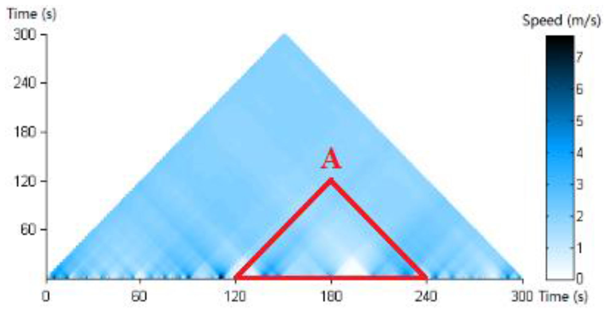
37] to represent continuous temporal data. The CTM has the ability to represent the attribute values during all time intervals. The attribute value during a time interval is calculated using a specific algebra operator (such as mean, summation and maximum) based on the attributes at the finest sampled time stamps within the time interval. The attribute values at the time stamps between any two neighboring sampled time stamps can be calculated using interpolation. Through color-coding, the continuous field of the CTM is displayed as an image, in which each color denotes the corresponding attribute value of a specific time interval. Hence, the color at a specific point in the CTM denotes the attribute value during a corresponding time interval. For example,
Figure 3 illustrates the values of the mean speed of a football player during the first five minutes of a game using the CTM. In
Figure 3, the value of the mean speed during any time interval within [2, 4] minutes corresponds to a specific point within triangle A.
In all, the CTM has a strong ability in visualizing temporal information at any temporal scale, from the finest till the coarsest. Therefore, it can be employed as a multi-temporal scale tool, by which meaningful information, which cannot be revealed by other tools, might be discovered. Based on these characteristics, the CTM is utilized in this paper to visualize the interaction patterns at multiple temporal scales so that useful information on dynamic interactions might be discovered [
12].
4. Case Study
4.1. Dataset
The movement data adopted in this paper come from a real and entire football match between ‘Club Brugge KV’ and ‘Standard de Liège’ which took place on 2 March 2014. For simplicity, we call them ‘Club Brugge’ and ‘Standard Liège’ respectively in the remainder of the paper. Football is considered as a highly interactive sport since the players need to interact (e.g., collaborate) frequently with the teammates. As such, various types of interaction patterns can be involved during a match. The exploration of player interactions is important as player interactions can give insight into a team’s playing style and can be used to assess the importance and performance of individual players of the team. In this dataset, the positions of all the players were tracked at a temporal resolution of 0.1 s. The data include both spatio-temporal information and semantic information. The spatio-temporal information is recorded in a (id, x, y, t) format, where id identifies a specific player, x and y represent the x and y coordinates of the player’s position, and t denotes the corresponding time stamp. The semantic information mainly includes the information of both teams, especially the basic information of the players (e.g., names, id numbers and positions played) and the events that happened during the match (e.g., event name, time of occurrence and id of the actors).
Note that Club Brugge won the match by 1-0 by scoring a goal at the time stamp 4733 s. As relatively more sophisticated interactions might be involved in a relatively short time interval before a goal event, the movement data of the players (except the goalkeeper) of Club Brugge during the time interval before and until the goal event are used as the experiment data. After checking the semantic information in the original data, time interval [4493, 4733] s is used since it contains many interesting events (e.g., shot events and free-kick events) just before the goal was scored. Besides, in order to reduce the computational complexity, we down-sampled the temporal resolution from 0.1 s to 1 s. Note that for reasons of simplicity, the time interval is changed to [0, 240] s from [4493, 4733] s. In addition, due to privacy issues, the actual names of the ten players are all replaced by player 1, player 2, player 3, …, and player 10.
4.2. Results and Analysis
4.2.1. The Interaction Intensities between Two Individuals for Each Interaction Pattern
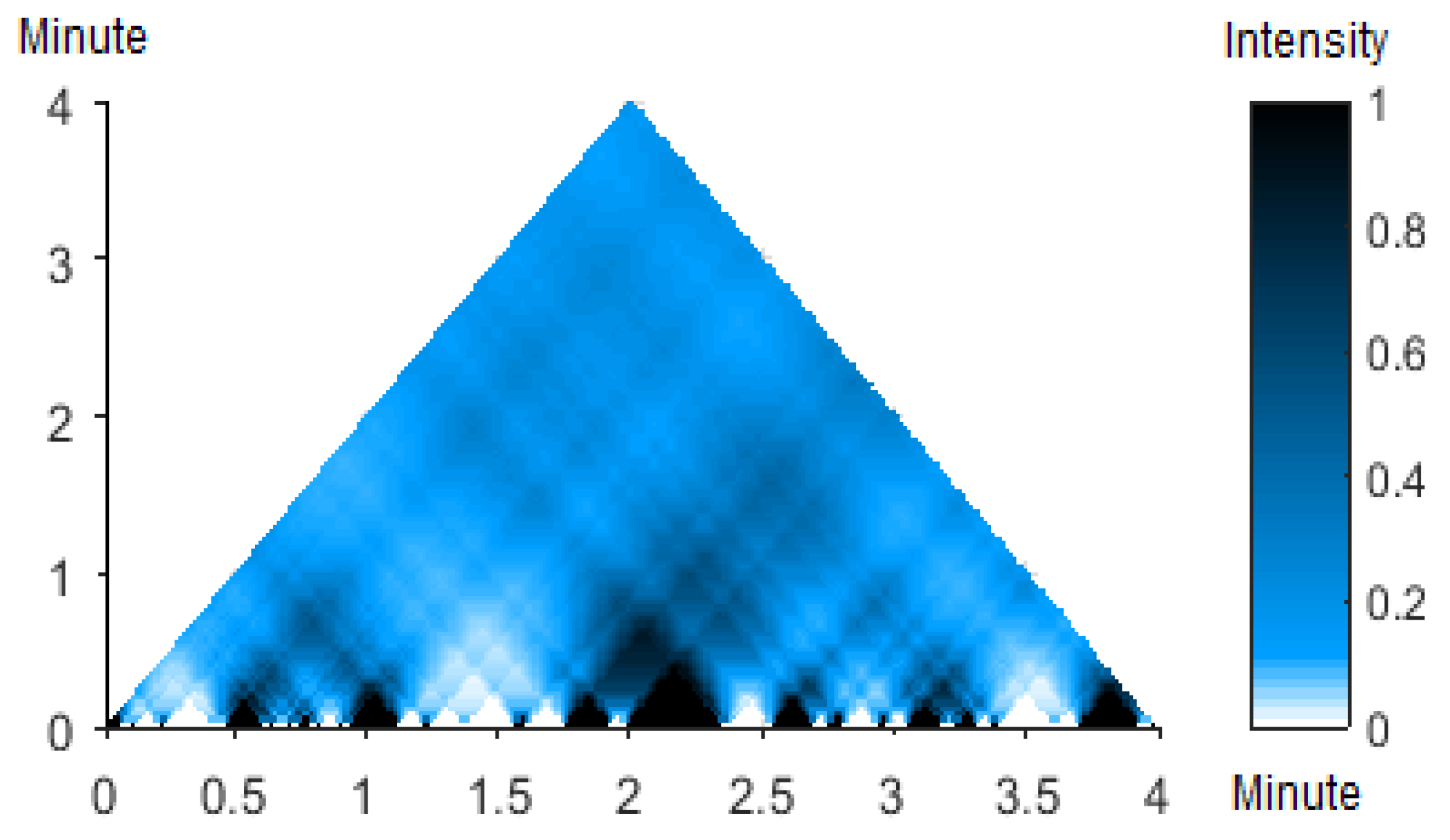
Based on the proposed approach, the interaction intensities between any two individuals during all time intervals for each interaction pattern can be explored. Take for instance the attraction pattern, the interaction intensities between player 1 and player 6 are shown in
Figure 5, in which a darker color denotes a stronger interaction and a lighter color corresponds to a weaker interaction. For example, according to
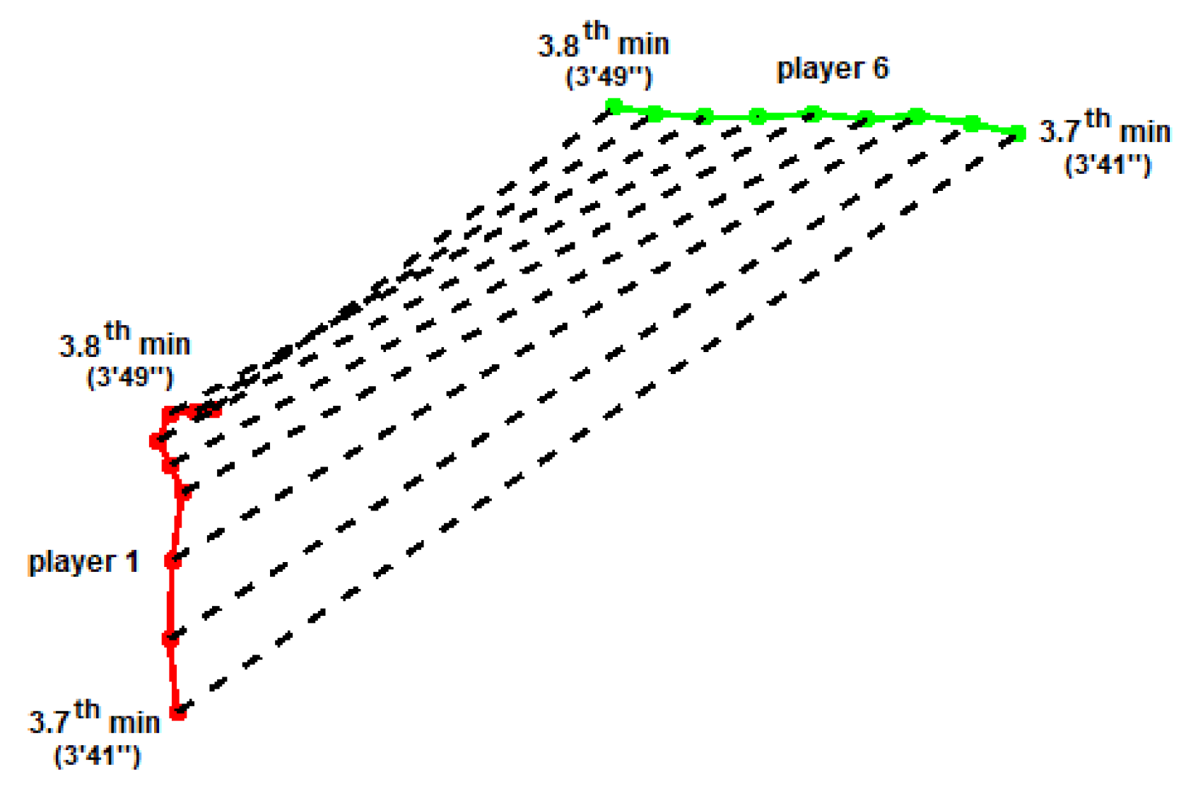
Figure 5, we can notice that the interactions between the two players during time interval just before the goal, [3.7, 3.8] min, were relatively strong. In order to validate this, we plotted the trajectories of the two players during this time interval, which is shown in
Figure 6, in which the red line denotes the trajectory of player 1, the green line the trajectory of player 6, and the black dotted line corresponds to the distance between the two players at each time stamp. Obviously, from
Figure 6, we can clearly see that the distance between player 1 and player 6 decreased during each time interval from the 3.7th minute to the 3.8th minute. One is thus able to explore the interactions between any two individuals based on the corresponding CTM diagrams according to the specific demands (e.g., particularly interested in the movements of players during a specific time interval by watching the video), after which the performance of a pair of players can be explored, which might be important to sports professionals (e.g., coaches).
4.2.2. The Interaction Intensities among Multiple Individuals for Each Interaction Pattern
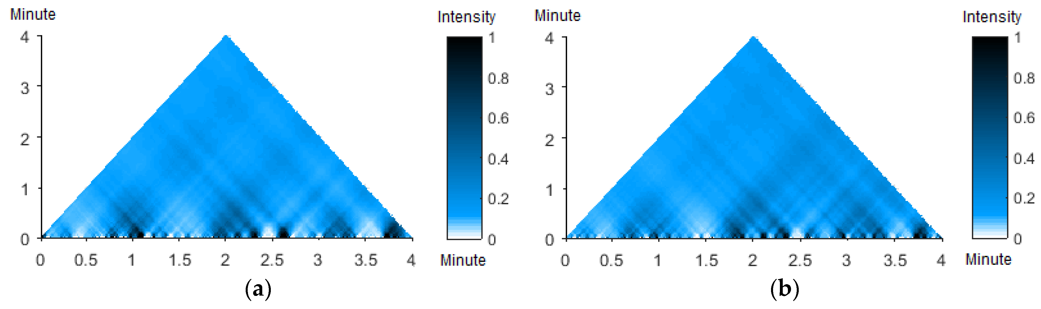
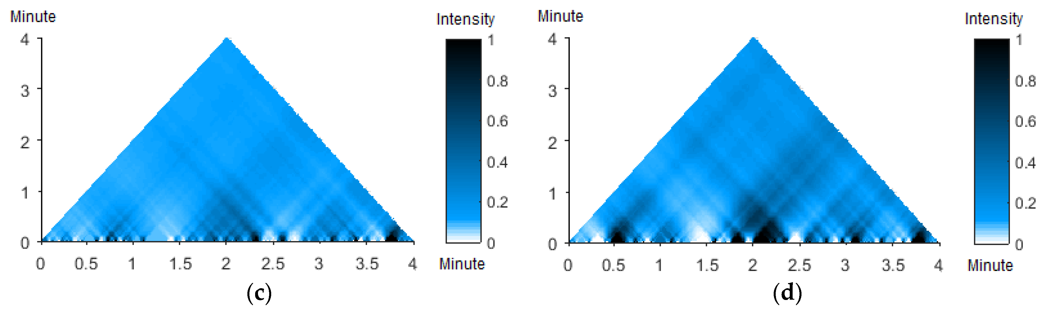
Under many circumstances, one individual might interact with more than one other individual. Specifically in team sports, tactics may involve multiple players simultaneously. For example, as the most fundamental aspect of a football match, the passing of the ball always involves multiple players. Thus, the exploration of the overall interaction intensities between one player and other players (i.e., the local interaction intensity of one player) is important to related sports professionals. This can be achieved using the proposed approach. By checking the dataset, we select four players (i.e., player 1, player 2, player 5 and player 6) as an illustration, since they were involved in a sequence of passes before the goal. Take the attraction pattern for example, the local interaction intensities of each player are shown in
Figure 7. From
Figure 7, we can observe that each player had time intervals during which his general interactions with others were relatively strong. For instance, by comparing
Figure 7a–d, we can find that during the time interval around [3.7, 3.8] min, the local interactions of each of the four players were all relatively strong, which indicates that each of them may collaborate well with the others during this time interval. When looking at the football match, we can see that this interval of strong local interactions coincides with spatial compression of these four players just before the goal.
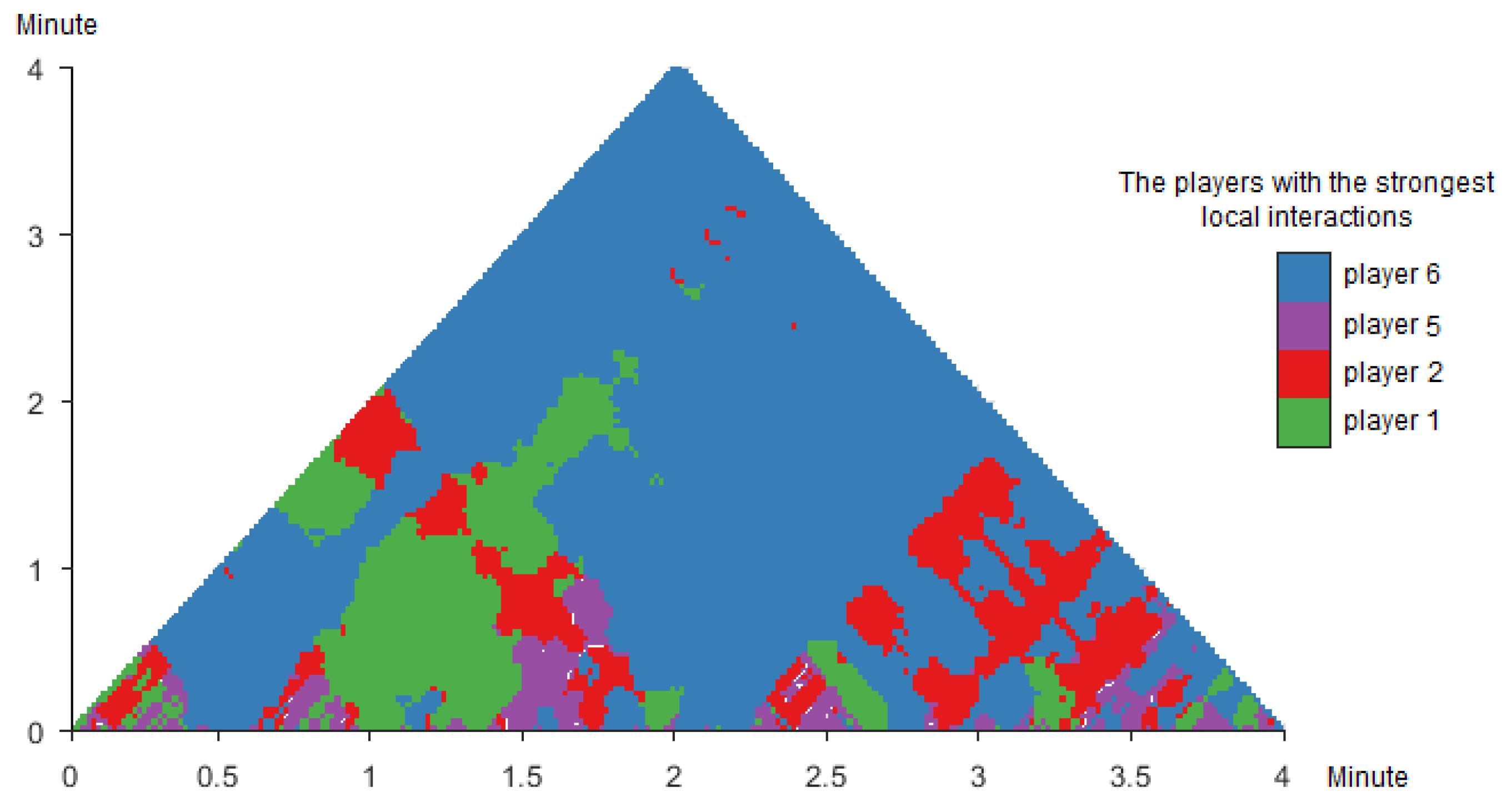
Besides, as introduced in [
12], by employing corresponding map algebra operations, additional information can be discovered. In this case, a new CTM diagram is generated by employing the ‘maximum’ operator to the four CTM diagrams displayed in
Figure 7. The new CTM diagram is shown in
Figure 8, in which each colour corresponds with a specific player.
Figure 8 depicts which player had the strongest local interactions during all time intervals. For instance, from
Figure 8, we can conclude that player 6 interacted comparatively more intensively with the other three players from the perspective of a long time-interval (e.g., longer than about 2.5 min). When the time intervals were shorter than about 2.5 min, each of the four players had specific time intervals during which he interacted comparatively more intensively with the other three players. This shows that, the proposed approach has potential to help sports professionals (e.g., coaches) to explore the local interactions of a group of target players in order to examine which player had a high influence on the movement patterns of the players around him, thus allowing evaluating player performance.
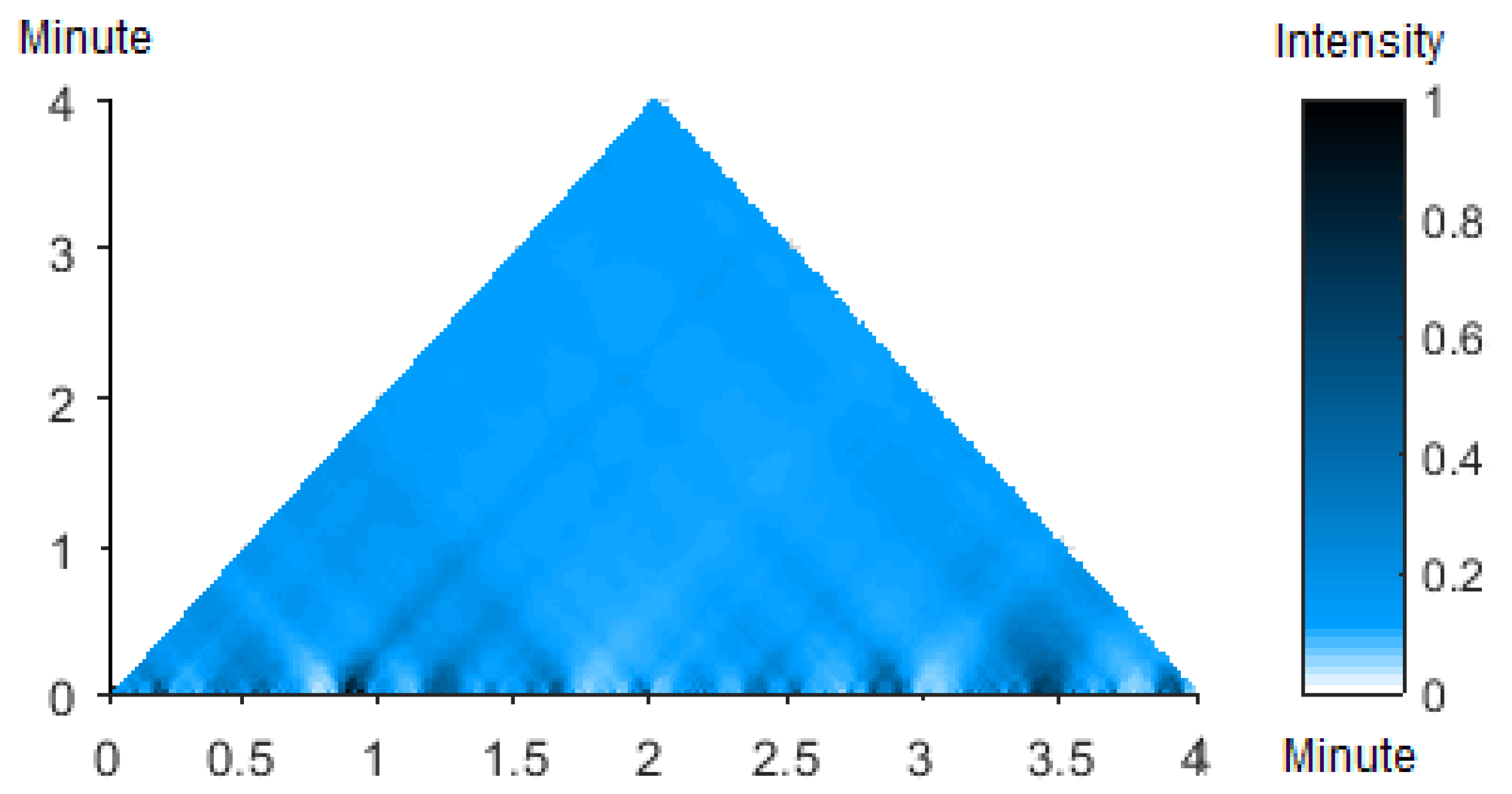
Apart from exploring the local interaction intensities of each individual for each interaction pattern, the approach can be used to explore the global interaction intensities of multiple individuals as well. This is particularly useful in team sports when examining the overall performance of multiple players. Take for instance all the ten players in a football match. When a team (e.g., team 1) possesses the ball, the players in the other team (e.g., team 2) tend to run towards each other to compress the space in order to tackle the opponents and to limit their options to pass the ball. Thus, for a good performance, the attraction pattern is expected to happen in team 2. On the contrary, the players of team 1 are expected to run away from each other in order to extend the space to pass the ball. Hence, for a good performance, the avoidance pattern is expected to happen in team 1. The overall performance of a team can be examined using the proposed approach by calculating the global interaction intensities among all the players. Take the avoidance pattern for instance, the global interaction intensities among all the players are shown in
Figure 9. In
Figure 9, for example, we can notice that the global interaction intensity values during time interval [0.85, 0.95] min were relatively large (which indicates that the overall interactions during this time interval were relatively strong), and the global interaction intensity values during time interval [2.95, 3.10] min were relatively small (which indicates that the overall interactions during this time interval were relatively weak). By checking the adopted dataset, we find that during time interval [0.85, 0.95] min, Club Brugge possessed the ball, thus the avoidance pattern was expected to occur in case of a good performance. This coincides well with the results during the corresponding time interval in
Figure 9, which demonstrates that Club Brugge indeed performed well generally during this time interval. On the other hand, during time interval [2.95, 3.10] min, Standard Liège possessed the ball. In case of a good performance, the attraction pattern was thus expected to happen for Club Brugge, which should make the overall interactions in the avoidance pattern weak during this time interval. Obviously, this coincides well with the results in
Figure 9 as well. Based on this, we can infer that Club Brugge also indeed had a good performance during this time interval. In terms of the simple analysis, we can conclude that the proposed approach has the ability to assist coaches to explore the overall interaction intensities among multiple players for each interaction pattern.
4.2.3. The Importance of Each Individual and the Identification of the Most Important Individuals in Each Interaction Pattern
The centrality measures can be used to measure the importance of an individual in an interaction pattern from different perspectives. In this case study, based on the centrality measures, the importance of each player for each interaction pattern can be evaluated, which might provide insightful information to coaches. Take player 6 and the attraction pattern for instance, the results of the centrality measures are visualized in
Figure 10. In
Figure 10, a dark color corresponds to a high value, which means that the player was a central player during the corresponding time intervals according to the corresponding centrality measure. Note that ‘central player’ here and hereafter means a player playing an important role according to centrality measures, but not a player who is located at the spatial center of the field. In
Figure 10, we can find that the importance of player 6 was different during all time intervals based on the same measure. For example, based on the measure of degree, player 6 can be considered as a central player during the time intervals which are dark, because player 6 had more direct connections with the other players in the MTSSTN during these time intervals. This indicates that the number of players whose distances between player 6 decreased during these time intervals was relatively large. Thus, player 6 had relatively good interactions with the other players for the attraction pattern and was considered a relatively central player of the movement pattern. Hence, based on the proposed approach, the importance of each player in each interaction pattern can be explored by using different centrality measures. This might provide potential insights to sports professionals and coaches for arranging suitable tactics and selecting the starting lineup for a match.
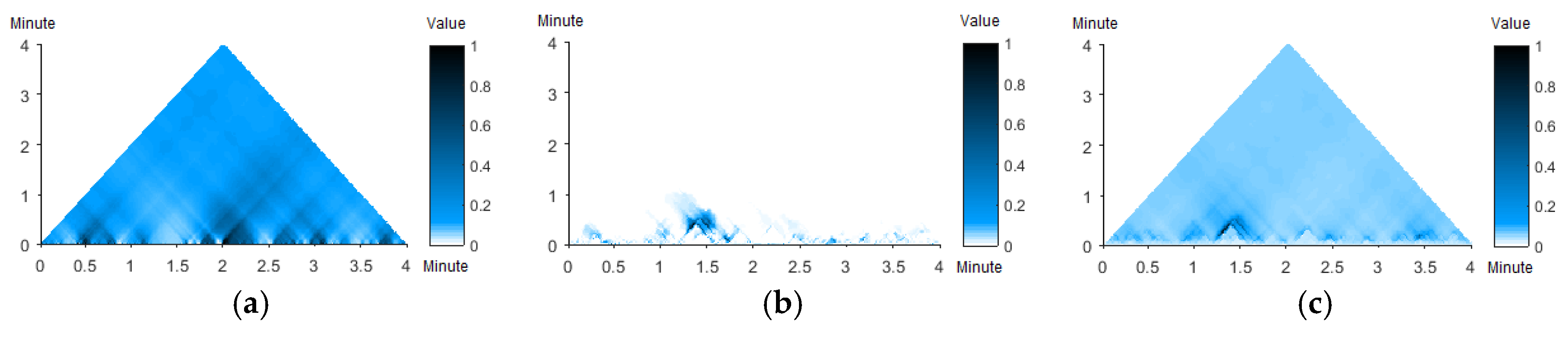
The identification of important individuals is of high importance since they might play rather important roles in specific types of interactions. In this case study, the most central players for each interaction pattern during all time intervals can be identified based on the proposed approach. This is achieved by employing corresponding map algebra operators (‘maximum’ in this case) to the corresponding CTM diagrams of the centrality measures of each player. The detailed principle can be seen in [
12]. The results are shown in
Figure 11. Note that in
Figure 11, similar colors are used for players at similar positions (i.e., players 1~3 are forward, players 4~6 midfielders and players 7~10 defenders).
Figure 11 clearly demonstrates which player was the most central player during which time interval for each interaction pattern based on different centrality measures. For instance, for the attraction pattern (
Figure 11a), player 4 can be considered as playing key roles based on degree and player 1 based on betweenness on a whole during relatively long time-intervals (e.g., longer than about 1 min). When the time intervals were shorter than 1 min, each player had his own dominant time intervals, during which this player was considered as a central player. Similarly, for the stability pattern, players 1, 3 and 5 can be considered as the most central players on a whole based on degree, players 1 and 8 the most central in general based on betweenness, and players 1, 3, 5 and 6 the most central generally based on closeness. For the avoidance pattern, obviously, player 1 was the most central player on a whole based on betweenness. From
Figure 11 we can observe that the results vary a lot, as in some of the figures, the most central players are quite easy to be identified, while in others this is not possible. However, one can draw specific conclusions by analyzing the corresponding figures in depth (e.g., zooming in the zone of a specific time interval on a CTM diagram) according to specific demands. Therefore, this approach has the potential to provide insightful suggestions to related sports professionals for suitable tactics arrangement and players’ performance evaluation.
5. Discussion
As a key contribution of this paper, we developed a hybrid approach combining the multi-temporal scale spatio-temporal network and the continuous triangular model and addressed the applicability of the approach in exploring dynamic interactions in movement data. Specifically, the approach is utilized in football movement data, a type of sports movement data which has gained much attention in recent years. The results showed that the proposed approach can be used to explore various interactions between the players. Besides, it is useful in evaluating the importance of each player and identifying the most central players.
As is known, scale is a common problematic issue in many disciplines, especially those that involve space and/or time (e.g., GIScience). In GIScience, scale is of significant importance. It even has been considered as the fifth dimension in 5D data modelling [
40]. Thus, it is crucial to take scale into consideration when dealing with space and/or time-related data. However, only limited research on dynamic interactions in movement data has taken scale (or in detail, temporal scale) into consideration. The research conducted by Long et al. [
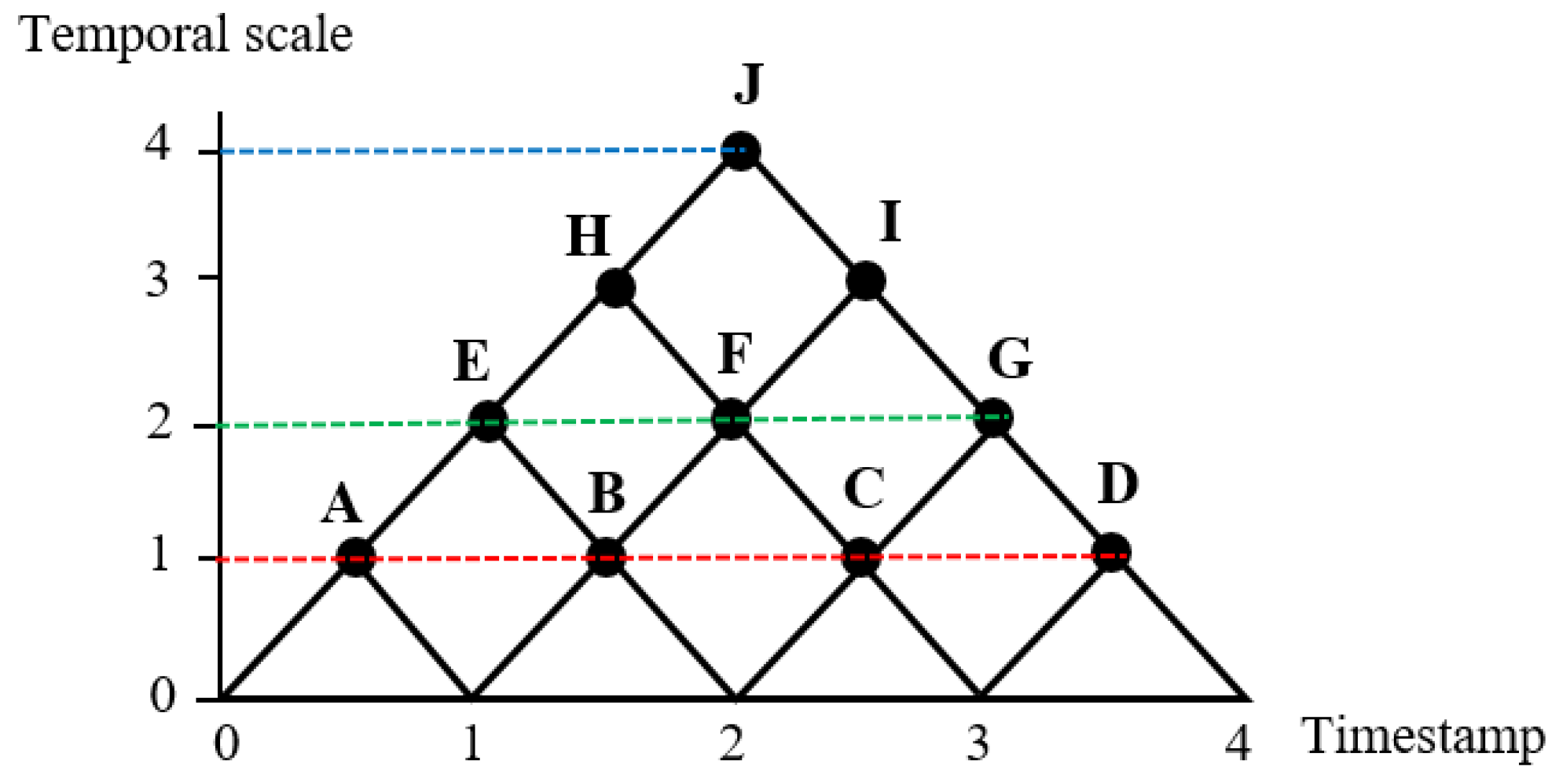
23] can be regarded as a typical example. In this research, it was argued that dynamic interactions can be analyzed from four analysis levels, i.e., local, interval, episodal and global. Local level is described as the finest temporal scale, interval level and episodal level correspond to a coarser temporal scale, and global level is considered as the coarsest temporal scale. A new computation has to be made if the analysis level changes, and new results have to be visualized correspondingly. Actually, the results at the four levels are contained simultaneously in the results of the proposed approach in this paper. In other words, the results at any of the four levels can be found in one corresponding CTM diagram. Take the simple CTM diagram in
Figure 12 for example, the
x-coordinate and
y-coordinate denote the time stamps and the temporal scales, respectively, the red dotted line and the blue dotted line indicate the local level and the global level, respectively, and the green dotted line either an interval level or an episodal level. Therefore, the values at points A, B, C and D correspond to the values at the local level, and the value at point J corresponds to the value at the global level. The values at the interval level can be found at points E, F and G, and the values at the episodal level can be found at points E and G. Hence, this approach appears to be superior in analyzing dynamic interactions at multiple temporal scales.
The dynamic interactions in movement data include both the interactions between a pair of individuals and the interactions among multiple (usually at least three) individuals. So far, current methods have mainly focused on the interactions between two individuals. However, it is common in practice to consider several objects as a group (e.g., four players as a moving flock). Hence, a method to explore the interactions among more than two individuals simultaneously is very much in need. Benefitting from the map algebra operations supported by the CTM, the proposed approach is capable to explore the interactions among multiple individuals. The results showed the effectiveness of this approach.
Network science provides a lot of powerful methods to study systems in the real world. Therefore, networks have been widely adopted as a useful tool to enable researchers to explore many systems in society, nature and technology. In the area of movement data analysis, networks have already been utilized as a tool as well. In recent time, a new type of network (i.e., spatio-temporal network) has been developed by Williams et al. [
32] in order to analyze spatio-temporal data more accurately. However, it appears unsatisfactory to analyze multi-temporal scale related issues. Based on this, in this paper, we propose an even more novel type of network (i.e., multi-temporal scale spatio-temporal network). To the best of our knowledge, this is the first case that adopted networks as a tool to analyze spatio-temporal data at multiple temporal scales. The results revealed the advantages of using the multi-temporal scale spatio-temporal network to discover insightful information that current networks cannot. We expect that the new type of network could be considered as a potential tool to gradually serve the domain of movement data analysis in the future.
However, the proposed approach still has its own flaws. On the one hand, although the interaction patterns derived based on RTC are prevalent between/among any two/multiple objects, they are still relatively simplistic. This, to some extent, limits the significance of the results exhibited during all time intervals in the case study. The results primarily make sense quite well during part of the time intervals, which are chosen by users (e.g., coaches) based on relevant information (e.g., the video of the match) according to their demands. In the future, more sophisticated interaction patterns might be derived using other potential methods automatically, such as qualitative trajectory calculus (QTC) [
41,
42,
43], dynamic interaction (DI) [
23] and relative motion (REMO) [
6], in order to enhance the meanings of results. On the other hand, the current approach appears costly in time (the complexity is O(
n3), where
n is the number of time intervals at the finest temporal scale), thus limiting its applicability for very large movement datasets, although it showed its applicability and usefulness in relatively small datasets (e.g., it took approximately 4 min in this case study on a Windows 10 system with a processor of 2.6 GHz and a RAM of 8 GB). Things thus need to be optimized in the future.
6. Conclusions and Future Work
Currently, movement data are collected in a variety of domains and are becoming a popular type of data. Although many research topics with respect to movement data have been undertaken, the research on dynamic interactions in movement data is still in its infancy. This paper proposes a hybrid approach combining the multi-temporal scale spatio-temporal network and the continuous triangular model to explore dynamic interactions in movement data. Four main steps are included in the approach: first, RTC is used to derive three interesting interaction patterns; second, a corresponding MTSSTN is generated for each interaction pattern; third, for each MTSSTN, both the interaction intensity measures and the three centrality measures—degree, betweenness and closeness—are computed; finally, the results are visualized using the CTM and analyzed based on the CTM diagrams. Based on the proposed approach, three distinctive aims regarding the dynamic interactions in movement data can be achieved at multiple temporal scales. The approach is then validated based on the movement data obtained from a real football match. The results demonstrate that the dynamic interactions involved in movement data can be explored effectively and useful information can be discovered based on the proposed approach.
In this paper, central to the approach is the construction of the MTSSTNs. For each interaction pattern, a corresponding MTSSTN can be generated. Networks include undirected or directed networks, and unweighted or weighted networks. As our aim is primarily methodological, in this paper, only unweighted undirected networks are generated. In the future, directed networks can be generated so that more insightful information might be revealed. Besides, in the proposed approach, the MTSSTN is generated only based on the spatio-temporal information involved in the movement data. In the future, the semantic information can also be employed to generate new types of MTSSTNs. For example, based on the passing information in football movement data, the multi-temporal scale spatio-temporal passing networks can be derived, according to which the dynamic interactions of football players regarding passing can be explored. In addition, the movement data from other domains can also be employed in order to extend the range of applications of the proposed approach.


