Uncertainty in Upscaling In Situ Soil Moisture Observations to Multiscale Pixel Estimations with Kriging at the Field Level

Abstract

Upscaling in situ soil moisture observations (ISMO) to multiscale pixel estimations with kriging is a key step in the comprehensive usage of ISMO and remote sensing (RS) soil moisture data. Scale effects occur and introduce uncertainties during upscaling processes because of spatial heterogeneity and the kriging method. A nested hierarchical scale series was established at the field level, and upscaled estimations at each scale were obtained by block kriging (BK) to illustrate multiscale ISMO upscaling processes. Those uncertainties were described with the results of comparison analysis against RS data, statistical analysis, and spatial trend surface analysis on multiscale estimations and were explained from the spatial heterogeneity perspective with a semivariogram analysis on ISMO. The results show that uncertainties exist and vary in multiscale upscaling processes, and the range of the empirical semivariogram could indicate scale effects. When the target scale is shorter than the range, BK maintains similar scale effects and global trends during upscaling processes, and the direct pixel estimation by BK is relatively close to the average of nested pixel estimations. This has great implications for understanding the kriging method in similar works.

1. Introduction

Soil moisture constitutes approximately 0.89% of the total quantity of water within the global hydrological cycle, but it is an important element of the hydrosphere, biosphere, and atmospheric water cycle [1,2]. Soil moisture significantly influences the partition of precipitation into infiltration, runoff, and evapotranspiration and benefits the analysis of the global water cycle and climatic variation [3,4,5]. When soil moisture is maintained at optimum levels, it supports risk reduction for crop science and minimizes nutrient leaching [6]. Thus, the acquisition and regulation of soil moisture datasets are important.

There are two primary ways to acquire spatiotemporal soil moisture data. With the improvements in sensor technologies and retrieval algorithms, spaceborne microwave remote sensing (RS) has become a powerful tool to retrieve soil moisture data at a large scale (e.g., regional and global levels) [7] and several satellite-based soil moisture products have been released [8,9,10]. Soil moisture products that are derived from the same satellite tend to be characterized by diverse resolutions to accommodate the diverse needs of different users, such as the Advanced Microwave Scanning Radiometer E (AMSR-E) for the Earth Observing System with spatial resolutions ranging from 5.4 to 56 km [8,11], the Advanced Scatterometer (ASCAT) with spatial resolutions ranging from 25 to 50 km [8,10,12], and the Soil Moisture Active Passive (SMAP) with spatial resolutions ranging from 10 km to 50 km [9,13]. And, with downscaling methods, some RS soil moisture products with high spatial resolution are also available for research at the field level. For example, soil moisture ocean salinity (SMOS) imagery has been downscaled to resolutions of 10 km, 4 km, or 1 km using moderate resolution imaging spectroradiometer (MODIS) data [14,15]. In addition, with the development of wireless communication techniques, the wireless sensor network (WSN) has been increasingly used to obtain in situ soil moisture observations (ISMO) in some projects [16,17,18,19]. ISMO with high temporal resolutions could provide accurate and credible estimations at observation sites, but the spatial extent would be limited; however, this limitation could be compensated for by using spaceborne microwave RS data. Hence, one significant issue of combining satellite-based soil moisture products with ground-based observations is the disparity in observation scales between the two types of data [20].

An upscaling method and a data assimilation strategy are necessary to convert multipoint WSN soil moisture observations to a pixel format covering the satellite footprint to eliminate this mismatch. There are four commonly used upscaling methods for in situ observations. The first and the most commonly used approach is the simple averaging of in situ data [21,22]. The second is to introduce a kriging algorithm while considering spatial autocorrelation [23]. The third approach is using distributed land surface modeling to simulate the spatial pattern of soil moisture [24], and the fourth approach is using the apparent-thermal-inertia-based method to derive the soil moisture from fine-resolution satellite thermal signals [19,22]. However, these four methods focus on the upscaling and validation of ISMO to the footprint of just one RS soil moisture product [20,22]. This leads to an obvious question that we want to answer: whether the upscaled results at different resolutions obtained by the same upscaling method are statistically comparable and spatially stable. If the answer is yes, that method will contribute to the data fusion of ISMO with multiresolution RS data as well. In addition, soil moisture is characterized by spatial–temporal heterogeneity, and this heterogeneity will change with the different soil texture, vegetation, topography, and meteorological conditions at different scales, adding uncertainty to the upscaling and validation processes [20,25,26]. How to quantitatively evaluate the scale effects in kriging from the perspective of spatial heterogeneity is another important question that we want to answer in this paper. Some researchers have realized the question and have done some simple descriptions in their works [27,28].

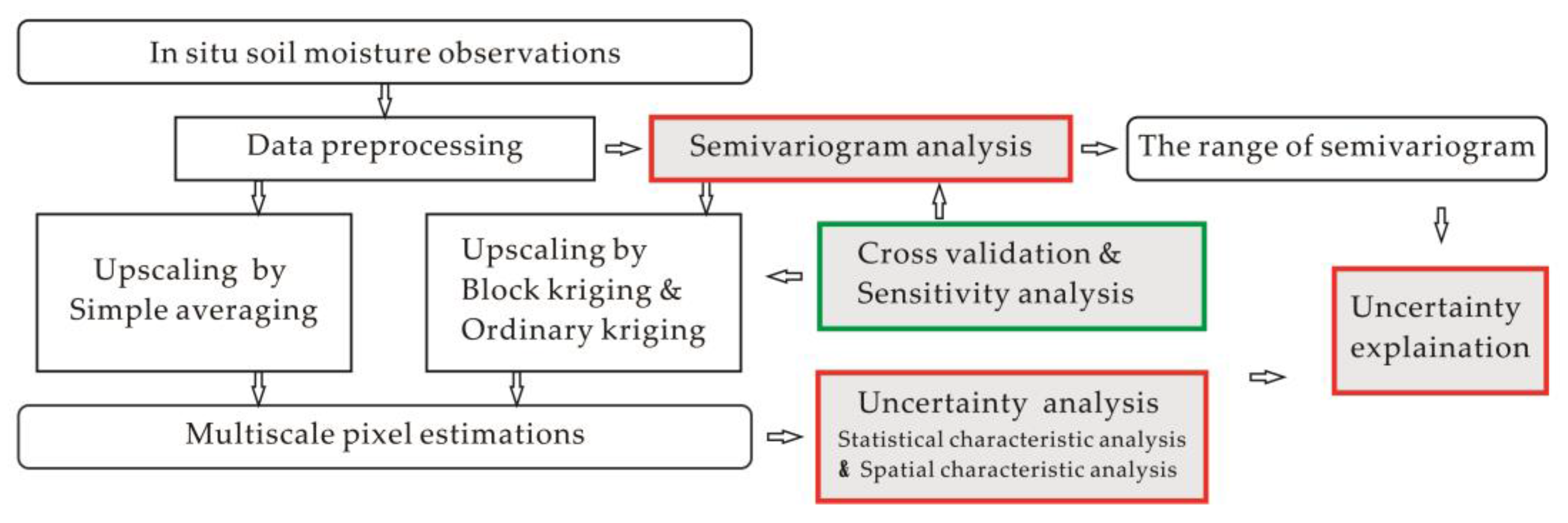
In this paper, we studied the two questions mentioned above to analyze statistical and spatial comparability and uncertainties in the upscaling processes of in situ soil moisture to multitarget scales and to explain the sources of uncertainties. We used block kriging (BK), a common geostatistical method used for soil moisture data [20,22,29], to upscale in situ soil moisture data, while ordinary kriging (OK) and simple averaging (SA) were used as contrasting methodologies. In addition, we utilized comparison analysis against RS data, statistical analysis, spatial trend surface analysis, and semivariogram analysis to describe and quantitatively evaluate the uncertainties in the upscaling processes. The remainder of this paper is organized as follows. Section 2 describes the data and the study area. Section 3 introduces the BK, OK, and SA upscaling methods for the soil moisture data at a variety of spatial scales and quantitatively evaluates the uncertainties occurring during the upscaling processes. The results are presented and discussed in Section 4 and Section 5, respectively. Key conclusions are drawn in the last section.

2. Data and Data Preprocessing

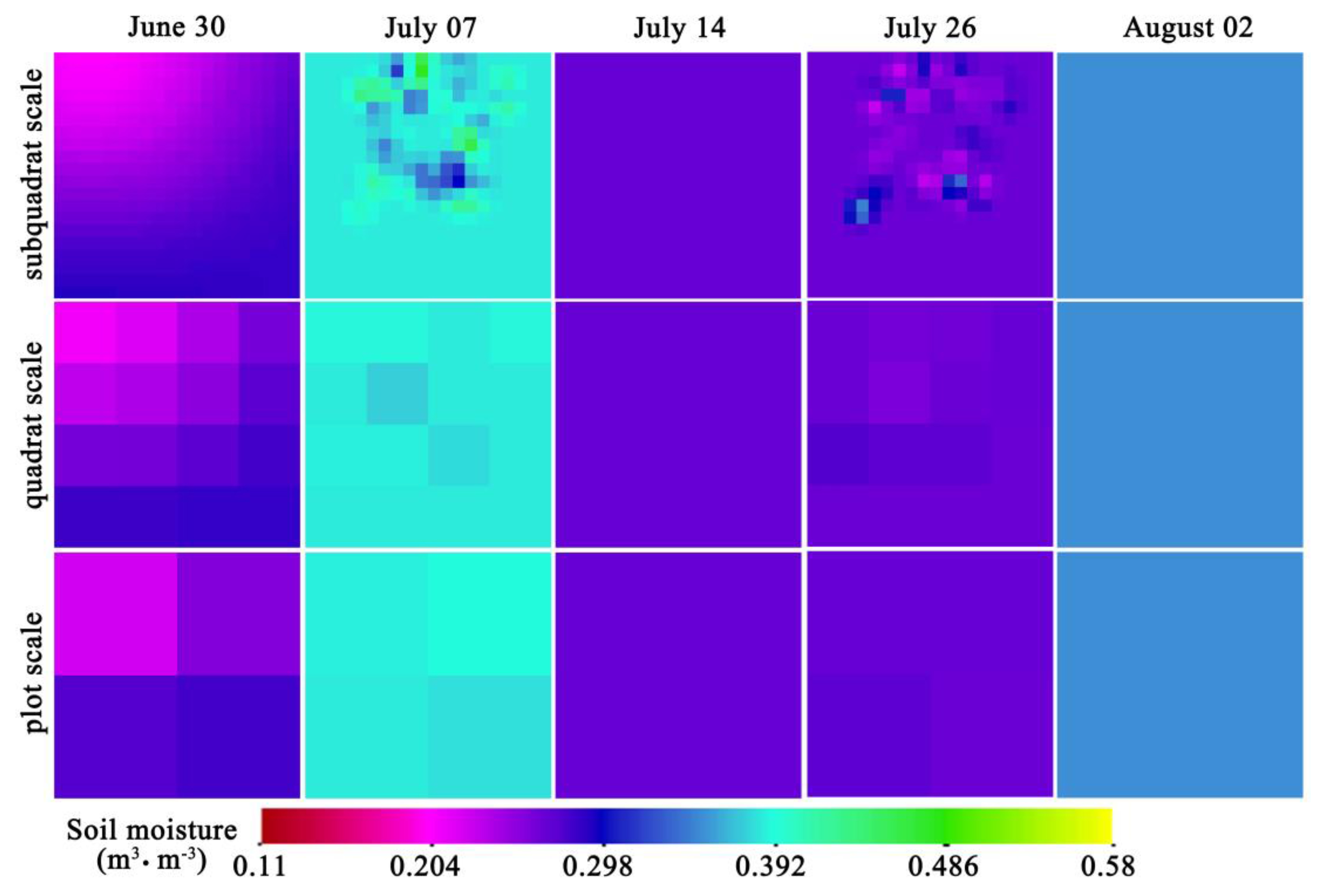
Datasets from the Heihe Watershed Allied Telemetry Experimental Research (HiWATER) project [17,30] were used in this study. The RS soil moisture data were extracted from a dataset of retrieved soil moisture products (5 cm depth) using airborne polarimetric L-band (1.4 GHz) multibeam radiometer (PLMR) brightness temperatures with 700 m spatial resolution on 30 June, 7 July, 14 July, 26 July, and 2 August 2012. The in situ soil moisture data were acquired from SoilNET observation data (4 cm depth) on 30 June, 7 July, 14 July, 26 July, and 2 August 2012 (synchronous with the PLMR data) [31,32,33].

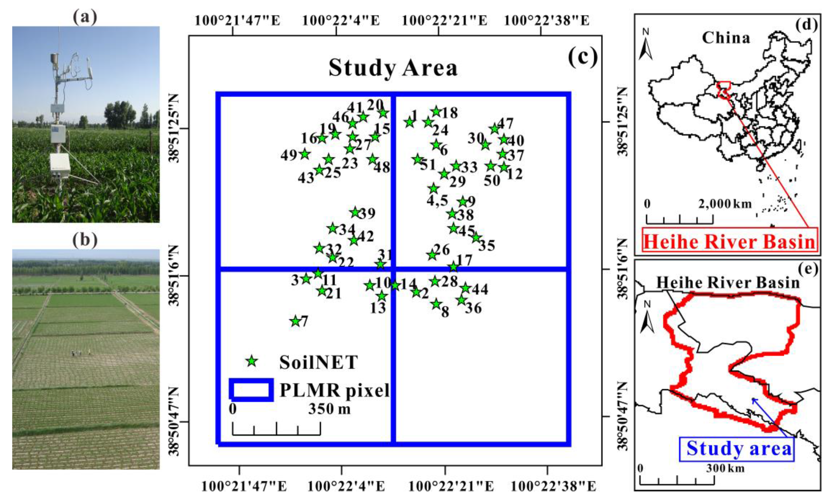
SoilNET is one of three WSN nodes (WaterNET, SoilNET, and BNUNET) adopted in the Ecological and Hydrological WSN (EHWSN) that uses optimal geostatistical sampling methods [32]. The EHWSN is located in both the Yingke and Daman irrigation districts of the Zhangye Artificial Oasis, where the irrigation system infrastructures are complete. The districts are in a typical semiarid and arid agricultural region and the main crop types are corn, wheat, vegetables, and fruits. In the districts, agricultural irrigation is essential for crop growth. Because of unscheduled agriculture irrigation, soil moisture has strong heterogeneity with complicated spatial processes [33]. Specifically, 51 SoilNET nodes designed by the Jülich Research Center [16] were used to capture the small-scale soil moisture variations, and the observations were covered by four (2 × 2) PLMR pixels. These four PLMR pixels represented the final study area in this study (Figure 1).

Because the RS soil moisture products were retrieved primarily by PLMR brightness temperature data, the PLMR flight time was selected as the reference time in this paper [34]. PLMR measured both V and H polarizations using a single receiver with polarization switching at incidence angles of ±7°, ±21.5°, and ±38.5° [17]. Therefore, there were several flight times in each PLMR pixel, and the temporal resolution of the in situ soil moisture data was 10 min. Therefore, all SoilNET data corresponding to all PLMR flight times in each PLMR pixel were averaged to guarantee data synchronicity and minimize errors.

Before the ISMO data were upscaled, a histogram and a Normal QQ plot were created using the exploratory data analysis tool in the Geostatistical Analyst toolbox of ESRI ArcGIS^® 10.4 software, and the outliers and data distributions were analyzed and processed to support the reliability and stability of the geostatistical methods [23,29,35]. The normal distribution was examined according to the kurtosis and skewness (both ideally close to 0) of the data on each date, supported by the Shapiro–Wilk test [35,36]. After careful scrutiny, nodes NO. 4, NO. 29, NO. 42, and NO. 47 were broken on multiple dates and were deleted as outliers on all dates [37,38] (Figure 2). Moreover, the SoilNET data on 26 July and on 2 August were not normally distributed. Thus, the logarithmic normalized transformations were conducted on those in situ observations of 26 July and of 2 August before using the kriging method, and back-transformations were conducted on the kriged results of 26 July and of 2 August.

3. Methodologies

A spatial scale series was established according to the PLMR resolution and the average distance between the SoilNET nodes and their nearest neighbors on each date to analyze the uncertainty in the upscaling process. BK, OK, and SA are common upscaling methods for soil moisture without any auxiliary data and were introduced to build the nested upscaled data series [22]. We used leave-one-out cross validation and sensitivity analysis to evaluate the kriging method and ensure its applicability at the field level in this study (Figure 3). With comparison analysis against RS data, statistical analysis, spatial trend surface analysis, and semivariogram analysis, the uncertainties were described and quantitatively evaluated.

3.1. Semivariogram and Upscaling Methods

Kriging is based on the theory and structural properties of a semivariogram, and it makes optimal and unbiased estimations for regionalized variables at unsampled locations [28,39]. A semivariogram is the basic of geostatistics, and can quantify the spatial heterogeneity of the regionalized variable, soil moisture $Z(x)$ [40,41]. The experimental semivariogram is defined as the following:

$$\gamma (h)=\frac{1}{2N(h)}{\displaystyle \sum _{\mathrm{i}=1}^{N(h)}{[Z(x_{\mathrm{i}})-Z(x_{\mathrm{i}}+h)]}^2}$$

(1)

where $N(h)$ is the number of pairs of observations separated by distance $h$. An empirical semivariogram can be approximated by predefined theoretical semivariogram models (e.g., pure nugget effect model, Gaussian model, exponential model, linear model, or spherical model) [19,23]. Three parameters—nugget, sill, and range—are often used to describe semivariograms. The nugget is the discontinuity of the semivariogram at the origin and can be used to judge if uncorrelated noise (measurement error) exists or if the spatial structures are smaller than the pixel size [42]. The sill indicates the spatial variability of the soil moisture [10,43]. The range is the distance at which the semivariogram reaches the sill and the distance beyond which the soil moisture has no spatial dependence [19]. Sometimes, some semivariograms approach their sills asymptotically, and so they have no strict ranges [35]. For practical purposes their effective ranges are usually taken as the lag distances at which they reach 0.95 of their sills. The empirical semivariograms on the five acquisition dates were calculated using ESRI ArcGIS^® 10.4 software with the best-fit criterion [29]. The way of choosing between competing semivariogram models is to evaluate their performance in the kriging interpolation [35].

The pixel estimations of soil moisture by BK and OK can be given by

$$Z(x)={\displaystyle \sum _{\mathrm{i}=1}^{\mathrm{n}}{\omega }_i\cdot Z\left(x_i\right)}$$

(2)

where ${\omega }_i$ is the weight coefficient of each soil moisture observation $x_i$. For OK, each weight coefficient ${\omega }_i$ is determined by

$$\left[\begin{array}{c}{\omega }_{\mathrm{i}}\\ \mu \end{array}\right]={\left[\begin{array}{cc}{\gamma }_{\mathrm{nn}}& 1\\ 1& 0\end{array}\right]}^{-1}·\left[\begin{array}{c}{\gamma }_{\mathrm{n}}\\ 1\end{array}\right]$$

(3)

where $\mu$ denotes Lagrange’s multiplier, ${\gamma }_{\mathrm{nn}}$ denotes the semivariogram values computed using the observation points, and ${\gamma }_{\mathrm{n}}$ denotes the semivariogram values computed using observation points and the points to be estimated [23,39]. For BK, each weight coefficient ${\omega }_{\mathrm{i}}$ is obtained from Equations (4) and (5):

$$\left[\begin{array}{c}{\omega }_{\mathrm{i}}\\ \mu \end{array}\right]={\left[\begin{array}{cc}{\gamma }_{\mathrm{nn}}& 1\\ 1& 0\end{array}\right]}^{-1}\cdot \left[\begin{array}{c}{\overline{\gamma }}_{\mathrm{n}}\\ 1\end{array}\right],$$

(4)

$${\overline{\gamma }}_{\mathrm{i}}=\frac{1}{|\mathrm{A}|}{\displaystyle \sum _{\mathrm{j}|\mathrm{j}\in \mathrm{A}}{\gamma }_{\mathrm{ij}}},$$

(5)

where ${\overline{\mathit{\gamma }}}_{\mathrm{n}}$ denotes the semivariogram value between block A and all observation points, which is the same as the average of the point-to-point semivariogram values between the observation points and the points to be estimated within A [23]. In other words, BK is a local average of OK, and it integrates the advantages of SA and OK. Hence, in former studies, BK was always taken as an improved method to SA for upscaling ISMO [22]. The upscaled soil moisture estimations (USME) at the scale series by BK and OK were calculated with the gstat package in R [44].

The applicability of semivariogram models and kriging to field-level interpolation was evaluated by leave-one-out cross-validation with the gstat package in R [44,45]. In this method, one station from the dataset is extracted as a verification point and its value is re-estimated with the kriging map created from remaining sample points and the semivariogram model. This process is repeated n (n equal to the number of sample points) times, and the residual is calculated each time. The mean error (ME), the mean squared error (MSE), and the mean squared deviation ratio (MSDR) are calculated and used to access the accuracy of the kriging model [35]. The ME is equal to the average of all residuals and is ideally close to 0. The MSE is equal to the average of the squared residuals and ideally small. The MSDR is equal to the average of all calculated ratios of the squared residual to the kriging variance [35]. If the model for the semivariogram is accurate, then the MSDR should be 1. Moreover, we conducted sensitivity analysis [46,47] on the predicted values and calculated associated MSE by changing the semivariogram model’s range within 10% of the original values in ESRI ArcGIS^® 10.4 software [48]. If the calculated MSE is small, then the kriging predictions based on the semivariogram model are robust and reliable.

The simple averaging method is the most direct upscaling method for soil moisture and is based on the assumption that the arithmetic mean of limited observations is representative for an area. In the simple averaging method, sampling errors are random and can be cancelled out [21,22]. The pixel estimations can be given by Equation (2), but each weight coefficient ${\omega }_i$ is determined by

$${\omega }_{\mathrm{i}}=\{\begin{array}{cc}{1/\mathrm{n}}_{\mathrm{i}},& Z(x_{\mathrm{i}})\in \mathrm{A}\\ 0,& \mathrm{otherwise}\end{array}$$

(6)

where ${\mathrm{n}}_{\mathrm{i}}$ is the number of soil moisture observations ${\mathrm{x}}_i$ within pixel A. This means that the pixel estimation is equal to the arithmetic mean of the soil moisture observations within that pixel. The USME by SA were implemented with the spatial join analysis tool in ArcGIS^® 10.4 software.

3.2. Spatial Scale Series

Plots, quadrats, and subquadrats are often regarded as sampling extent indices in agriculture science and ecology [49], and these indices are introduced to represent the scale series. The scale series covers the entire study area (1400 × 1400 m). The plot scale consists of 4 grids of the same size (700 × 700 m), the quadrat scale consists of 16 grids of the same size (350 × 350 m), and the subquadrat scale consists of 400 grids of the same size (70 × 70 m). The plot scale and the PLMR products are of the same size. The length of the subquadrat scale is similar to the average distance between the SoilNET nodes and their nearest neighbors on each date (~70 m).

The spatial scale series illustrates the nesting relation of an even hierarchy [50,51]. Based on that, the regression relation between the in situ data and the scale series can be established to answer the two questions mentioned above. The USME at the plot scale (p), the quadrat scale (q), and the subquadrat scale (s) can be achieved by

$${\theta }_i^{\mathrm{p}}=U_{\uparrow }\left({\mathit{\theta }}^{\mathrm{situ}}\right),i=1,2,3,4$$

(7)

$${\theta }_j^{\mathrm{q}}=U_{\uparrow }\left({\mathit{\theta }}^{\mathrm{situ}}\right),j=1,2,\cdots ,16$$

(8)

$${\theta }_k^{\mathrm{s}}=U_{\uparrow }\left({\mathit{\theta }}^{\mathrm{situ}}\right),k=1,2,\cdots ,400$$

(9)

$${\mathit{\theta }}^{\mathrm{situ}}={\left[{\theta }_1{}^{\mathrm{situ}},{\theta }_2{}^{\mathrm{situ}},\cdots ,{\theta }_{\mathrm{n}}{}^{\mathrm{situ}}\right]}^{\mathrm{T}},\mathrm{n}=1,2,\dots ,47$$

(10)

where $U_{\uparrow }(·)$ denotes the upscaling methods corresponding to BK, OK, and SA in this paper and ${\theta }^{\mathrm{situ}}({\mathrm{m}}^3\cdot {\mathrm{m}}^{-3})$ denotes the preprocessed SoilNET soil moisture data.

3.3. Uncertainties Occurring in the Upscaling Processes to a Scale Series

3.3.1. Comparison of Upscaled Pixel Soil Moisture Estimations to Remote Sensing Data

The unstable spatial–temporal heterogeneity in soil moisture will introduce uncertainties into upscaling for validation activities of USME to RS data [27,52,53]. Given the lack of multiresolution RS data, only the plot scale and PLMR products are of the same size, and the PLMR footprint is regarded as one of the target scales in the upscaling process. Thus, the USME at the plot scale (p) is compared with the RS data using the root mean squared error (RMSE) to explore uncertainties in upscaling processes, which is expressed as $\mathit{RMSE}({\mathit{\theta }}^{\mathrm{P}},{\mathit{\theta }}^{\mathrm{RS}})$ [18,20,27].

3.3.2. Statistical Characteristic Analysis for Multiscale Pixel Estimations

The statistical characteristics of the USME between different scales can be represented by several statistical indicators, e.g., standard deviation, arithmetic average, median, and pixel center value. A modified standard deviation and arithmetic average are adopted in this paper (Figure 4). To verify the comparability between the USME at the larger scale (LS) and those at the smaller scale (SS), the arithmetic average of the USME of the SS pixels encapsulated in each LS pixel is calculated as ${({\overline{\mathit{\theta }}}^{\mathrm{SS}})}^{\mathrm{LS}}$. The ${({\overline{\mathit{\theta }}}^{\mathrm{SS}})}^{\mathrm{LS}}$ is compared to the actual USME of the LS pixel (${\mathit{\theta }}^{\mathrm{LS}}$) using the RMSE, and the comparison is expressed as $\mathit{R}\mathit{M}\mathit{S}\mathit{E}({\mathit{\theta }}^{\mathrm{LS}},{({\overline{\mathit{\theta }}}^{\mathrm{SS}})}^{\mathrm{LS}})$.

The modified standard deviations of USME at the SS within each LS pixel are expressed as ${\mathit{S}\mathit{D}}^{\mathrm{LS}}({\mathit{\theta }}^{\mathrm{SS}})$. ${\mathit{S}\mathit{D}}_i^{\mathrm{LS}}({\mathit{\theta }}_j^{\mathrm{SS}})$ is derived from the standard deviation, and is obtained by

$$\mathit{S}{\mathit{D}}_i^{\mathrm{LS}}({\mathit{\theta }}_j^{\mathrm{SS}})=\sqrt{{\displaystyle \sum _j{({\mathit{\theta }}_j^{\mathrm{SS}}-{\mathit{\theta }}_i^{\mathrm{LS}})}^2}/(n-1)}$$

(11)

where ${\mathit{S}\mathit{D}}_i^{\mathrm{LS}}({\mathit{\theta }}_j^{\mathrm{SS}})$ denotes the calculated deviations of the SS pixels USME within the LS pixel $i$, ${\mathit{\theta }}_j^{\mathrm{SS}}$ denotes the SS pixel $j$ within the LS pixel $i$, and $n$ is the number of the SS pixels in each LS pixel. The ${\mathit{S}\mathit{D}}_i^{\mathrm{LS}}({\mathit{\theta }}_j^{\mathrm{SS}})$ within each LS pixel are compared with each other and the differences are ideally small. The smaller the differences of deviations among these LS pixels, the more consistent the scale effects of the different regions. Moreover, if ${\mathit{S}\mathit{D}}_i^{\mathrm{LS}}({\mathit{\theta }}_j^{\mathrm{SS}})$ is ideally small, it indicates negligible difference between the LS pixel $i$ and the SS pixels within pixel $i$. In this paper, the LS and SS groups are plot–quadrat, plot–subquadrat and, quad–subquadrat (Figure 4). ${\mathit{S}\mathit{D}}_i^{\mathrm{p}}({\theta }_j^{\mathrm{q}})$ denotes the calculated deviations of the quadrat pixel USME within the plot pixel $i$.

3.3.3. The Spatial Characteristic Analysis for Multiscale Pixel Estimations and In Situ Soil Moisture

A trend surface analysis is a mathematical method used to fit the spatial distribution and spatial variation trends of regionalized variable $Z(x)$ by fitting a binary regression equation and using the least squares method [35,55,56]. Then, the observation surface of the regionalized variable is decomposed into a component associated with any regional trend and a residual associated with the purely local effect. In this paper, the linear trend surface is fitted to describe the global spatial variation trend of the ISMO, and that of the USME at each scale and can be expressed as

$$Z=b_0+b_{1}x+b_{2}y$$

(12)

where $x$ and $y$ denote the coordinates of the regionalized variables, and $b$ is the coefficient of the binary linear regression equation. For the analysis of the USME at each scale, the regionalized variables are the center points of each pixel at each scale, and the attribute values are the USME of the grids at each scale. For analysis of the ISMO, the regionalized variables are the SoilNET data. A measure of the significance of the increases in the fit level is the F ratio, which is formulized as

$$F=\frac{S{S}_{\mathrm{R}}/p}{S{S}_{\mathrm{D}}/(n-p-1)}$$

(13)

where $S{S}_{\mathrm{D}}$ denotes the residual sum of squares, $S{S}_{\mathrm{R}}$ equals the regression sum of squares, $n$ denotes the number of regionalized variables, and $p$ denotes the degree of freedom. For the analysis of the USME at each scale, $n$ corresponds to the number of grids at each scale. For the analysis of the ISMO, $n$ corresponds to the quantity of remaining 47 SoilNET nodes on each date after the removal of four outliers. Under the conditions of the F test, similar coefficients of the binary linear regression equations indicated more consistent global spatial trends [57].

4. Results

4.1. Semivariogram Analysis of the In Situ Soil Moisture Data and Upscaled Soil Moisture Estimations

Gaussian model, spherical model, and exponential model were chosen as the candidate models for they are widely used in soil research [58,59]. From the performance shown in

Table 1. Cross-validation of kriging on SoilNET soil moisture observations. ME (m³·m⁻³): the mean error. MSE (m³·m⁻³)²: the mean squared error. MSDR: the mean squared deviation ratio.

Semivariogram Model	Evaluation Indicator	Acquisition Time
		30 June	7 July	14 July	26 July	2 August
Exponential	ME	0.0006	0	-	0.0021	-
	MSE	0.003	0.006	-	0.049	-
	MSDR	1.34	1.99	-	2.48	-
Gaussian	ME	0.0004	−0.0002	-	0.0004	-
	MSE	0.003	0.006	-	0.049	-
	MSDR	1.24	1.3	-	1.67	-
Spherical	ME	0.0009	−0.0002	-	0.0003	-
	MSE	0.003	0.005	-	0.038	-
	MSDR	1.21	0.93	-	1.02	-
Pure Nugget	ME	-	-	−0.0002	-	0
	MSE	-	-	0.005	-	0.022
	MSDR	-	-	0.93	-	1.03

, we selected a Gaussian model for 30 June, a Spherical model for 7 July and 26 July, and a pure nugget model for 14 July and 2 August (Figure 5).

Besides this, three random range values were found that were within 10% of the model range to check the sensitivity of the model to the range (

Table 2. Semivariogram sensitivity analysis to the model range (m) on 30 June, 7 July, and 26 July with indicator, MSE (m³·m⁻³)²: the mean squared error.

Gaussian/30 June		Spherical/7 July		Spherical/26 July
Range	MSE	Range	MSE	Range	MSE
1102.7	0.01458	127.8	0.01347	120.5	0.00489
1241.6	0.01418	147.6	0.03364	124.4	0.01219
1251.7	0.01416	152.2	0.03488	145.8	0.02293

). For the Gaussian model on 30 June, the kriging was not sensitive to a larger range, whereas for the Spherical model on 14 July and 26 July, the kriging was not sensitive to a smaller range. Hence, the fitted range of the empirical semivariogram model in this paper is reliable (Figure 5). The range on 30 June was longer than 1179.7 m, which means that the SoilNET data were spatially homogeneous within the study area on that day (Figure 5). The ranges on 7 July and 26 July were shorter than 140 m, which means that the SoilNET data were spatially heterogeneous within the study area on those days. The ranges on 14 July and 2 August were 0, and indicate that the SoilNET data did not reveal the characteristics of autocorrelation on these two days.

The variability of the USME based on BK and OK was roughly consistent at each scale on 30 June (

Table 3. Coefficients of variation of upscaled soil moisture estimations at the scale series on five acquisition dates. Sub: subquadrat scale. Quad: quadrat scale. Plot: plot scale.

Coefficient of Variation (%)	Block Kriging			Ordinary Kriging			Simple Averaging
	Sub	Quad	Plot	Sub	Quad	Plot	Sub	Quad	Plot
30 June	9.87	9.88	9.98	9.88	10.13	11.09	23.11	13.81	10.44
7 July	3.99	0.89	0.98	4.45	4.40	2.77	17.10	9.49	5.93
14 July	0	0	0	0	0	0	16.28	5.99	7.17
26 July	4.15	1.32	0.45	4.74	3.44	4.51	19.22	11.67	8.01
2 August	0	0	0	0	0	0	15.22	10.16	3.93

, Figure 6 and Figure 7). The variability of the USME by BK declined with decreasing spatial resolutions on 7 July and 26 July. On 14 July and 2 August, the soil moisture estimations upscaled by BK and OK were fixed-value at all scales (Figure 6 and Figure 7). However, the variability of the USME by SA decreased overall with the decreasing spatial resolution on all acquisition dates (Table 3, Figure 8).

4.2. Uncertainties Occurring in the Upscaling Processes to the Scale Series

4.2.1. Statistical Characteristics of Multiscale Pixel Estimations

The $\mathit{R}\mathit{M}\mathit{S}\mathit{E}({\mathit{\theta }}^{\mathrm{LS}},{({\overline{\mathit{\theta }}}^{\mathrm{SS}})}^{\mathrm{LS}})$ values based on BK on 30 June, 14 July, and 2 August and those based on OK on 14 July and 2 August were close to 0 (

Table 4. Comparison of the upscaled soil moisture estimations of the larger scale (LS) pixels and the averaged value of the smaller scale (SS) pixel estimations within each LS pixel based on block kriging, ordinary kriging, and simple averaging and using root mean squared error (RMSE): $\mathit{R}\mathit{M}\mathit{S}\mathit{E}({\theta }^{\mathrm{LS}},{({\overline{\theta }}^{\mathrm{SS}})}^{\mathrm{LS}})$ (m³·m⁻³).

Upscaling Method	$\mathit{R}\mathit{M}\mathit{S}\mathit{E}({\mathit{\theta }}^{\mathbf{LS}},{({\overline{\mathit{\theta }}}^{\mathbf{SS}})}^{\mathbf{LS}})$	Acquisition Time
		30 June	7 July	14 July	26 July	2 August
Block Kriging	$\mathit{R}\mathit{M}\mathit{S}\mathit{E}({\theta }^{\mathrm{p}},{({\overline{\theta }}^{\mathrm{q}})}^{\mathrm{p}})$	0	2.81·10−3	0	2.87·10−3	0
	$\mathit{R}\mathit{M}\mathit{S}\mathit{E}({\theta }^{\mathrm{p}},{({\overline{\theta }}^{\mathrm{s}})}^{\mathrm{p}})$	0	3.06·10−3	0	2.81·10−3	0
	$\mathit{R}\mathit{M}\mathit{S}\mathit{E}({\theta }^{\mathrm{q}},{({\overline{\theta }}^{\mathrm{s}})}^{\mathrm{q}})$	0	7.92·10−4	0	5.54·10−4	0
Ordinary Kriging	$\mathit{R}\mathit{M}\mathit{S}\mathit{E}({\theta }^{\mathrm{p}},{({\overline{\theta }}^{\mathrm{q}})}^{\mathrm{p}})$	2.52·10−3	1.02·10−2	0	1.05·10−2	0
	$\mathit{R}\mathit{M}\mathit{S}\mathit{E}({\theta }^{\mathrm{p}},{({\overline{\theta }}^{\mathrm{s}})}^{\mathrm{p}})$	2.52·10−3	1.04·10−2	0	1.07·10−2	0
	$\mathit{R}\mathit{M}\mathit{S}\mathit{E}({\theta }^{\mathrm{q}},{({\overline{\theta }}^{\mathrm{s}})}^{\mathrm{q}})$	6.19·10−4	1.79·10−2	0	9.57·10−3	0
Simple Averaging	$\mathit{R}\mathit{M}\mathit{S}\mathit{E}({\theta }^{\mathrm{p}},{({\overline{\theta }}^{\mathrm{q}})}^{\mathrm{p}})$	7.90·10−3	1.19·10−2	1.41·10−3	6.55·10−3	1.25·10−2
	$\mathit{R}\mathit{M}\mathit{S}\mathit{E}({\theta }^{\mathrm{p}},{({\overline{\theta }}^{\mathrm{s}})}^{\mathrm{p}})$	1.01·10−3	1.04·10−3	7.73·10−4	5.95·10−4	2.40·10−4
	$\mathit{R}\mathit{M}\mathit{S}\mathit{E}({\theta }^{\mathrm{q}},{({\overline{\theta }}^{\mathrm{s}})}^{\mathrm{q}})$	1.05·10−3	1.82·10−3	1.88·10−3	1.14·10−3	1.20·10−3

). However, the $\mathit{R}\mathit{M}\mathit{S}\mathit{E}({\mathit{\theta }}^{\mathrm{LS}},{({\overline{\mathit{\theta }}}^{\mathrm{SS}})}^{\mathrm{LS}})$ values based on BK on 7 July and 26 July, those based on OK except on 14 July and 2 August, and those based on SA on all acquisition dates were relatively far from 0. At the same time, the SoilNET soil moisture was relatively homogeneous on 30 June, while it had no spatial autocorrelation on 14 July and 2 August (Figure 5). These results mean that the actual USME by BK of each LS pixel was close to the arithmetic average of those of the SS pixels within each LS pixel when the SoilNET soil moisture data were spatially homogeneous within the scale series. When the ISMO were spatially heterogeneous or not spatially autocorrelated within the scale series, this conclusion may not be true. Moreover, the actual USME by OK and SA showed similar characteristics but not as apparent as those by BK.

The differences of ${\mathit{SD}}^{\mathrm{LS}}({\mathit{\theta }}^{\mathrm{SS}})$ among all pixels at the LS are shown in boxplots to analyze the scale effects of the different regions (different pixels at the LS) in the upscaling process (Figure 9). The degrees of variation of ${\mathit{SD}}^{\mathrm{LS}}({\mathit{\theta }}^{\mathrm{SS}})$ based on BK and OK were less significant than those based on SA, proving the improvements of BK to SA. At the same time, the degrees of variation of ${\mathit{SD}}^{\mathrm{LS}}({\mathit{\theta }}^{\mathrm{SS}})$ based on OK are relatively significant compared with those based on BK (Figure 9a,b). This shows the better performance of BK than OK in keeping the scale effects with different datasets. Moreover, from the point of the comparison between the degrees of variation of ${\mathit{SD}}^{\mathrm{LS}}({\mathit{\theta }}^{\mathrm{SS}})$ on 30 June and those on 7 July or 26 July based on kriging, the scale effects of USME by kriging remained consistent among the different regions during the upscaling process when the SoilNET soil moisture data were spatially homogeneous within the scale series.

4.2.2. Spatial Characteristics of Multiscale Pixel Estimations

The trend surface derived from the SoilNET ISMO was only significant (p < 0.05, the null hypothesis of no trend was rejected) on 30 June. The trend surfaces based on the USME by BK at the subquadrat and quadrat scales were also significant and the coefficients b₀, b₁, and b₂ of the binary linear regression equations at the scale series were similar (

Table 5. The coefficients (b₀, b₁, b₂) of the binary linear regression equation for the trend surface analysis based on the in situ SoilNET soil moisture observations and the upscaled soil moisture estimations by block kriging, ordinary kriging, and simple averaging, and the F ratio on 30 June. F_0.05 is the F value with the significance level of 0.05.

Method	Scale	b0	b1	b2	F Ratio	F0.05
Block Kriging	Sub Quadrat	209.049	2.78·10−5	−5.25·10−5	1511.888	3.018
	Quadrat	210.577	2.81·10−5	−5.29·10−5	55.970	3.806
	Plot	215.719	2.89·10−5	−5.43·10−5	6.130	199.5
Ordinary Kriging	Sub Quadrat	209.236	2.79·10−5	−5.26·10−5	1510.231	3.018
	Quadrat	215.397	2.88·10−5	−5.42·10−5	54.433	3.806
	Plot	237.246	3.21·10−5	−5.97·10−5	5.442	199.5
Simple Averaging	Sub Quadrat	287.184	5.50·10−5	−7.46·10−5	4.638	3.214
	Quadrat	264.256	1.91·10−5	−6.17·10−5	1.461	5.143
	Plot	181.088	1.94·10−5	−4.48·10−5	0.667	199.5
SoilNET		288.629	5.84·10−5	−7.55·10−5	4.846	3.209

). Analogously, the trend surfaces based on the USME by OK presented similar trend surfaces, whereas at the same scale, the F ratio values computed for the trend surface derived from the USME based on BK were greater than those based on OK. These results indicate that the USME based on kriging could keep the global trend in the data, and, as the scale decreased, the ability of BK to maintain a similar global trend was relatively stronger than that of OK. By comparison, the trend surfaces derived from the SoilNET ISMO on 7 July, 14 July, 26 July, and 2 August were not significant (p > 0.05, the null hypothesis of no trend was accepted), and the trend surfaces based on the USME by kriging and SA on these days were also not significant.

4.2.3. Comparison between Upscaled Soil Moisture Estimations and Remote Sensing Data

The USME by BK, OK, and SA were relatively most close to the PLMR data on 30 June (Figure 10). The calculated RMSE values based on BK, OK, and SA on 30 June were relatively lower than those on other acquisition days (

Table 6. Comparison of upscaled soil moisture estimations at plot scale ${\theta }^{\mathrm{P}}$ against remote sensing data ${\theta }^{\mathrm{RS}}$ using root mean square error (RMSE).

$\mathit{R}\mathit{M}\mathit{S}\mathit{E}({\mathit{\theta }}^{\mathbf{P}},{\mathit{\theta }}^{\mathbf{RS}})$ (m3·m−3)	Acquisition Time
	30 June	7 July	14 July	26 July	2 August
Block Kriging	0.036	0.149	0.066	0.040	0.143
Ordinary Kriging	0.036	0.149	0.066	0.041	0.143
Simple Averaging	0.035	0.132	0.053	0.047	0.135

). These results indicate that the soil moisture estimations upscaled by BK, OK, or SA to the RS footprints with in situ data were not always similar with the RS data and may not even be able to calibrate them. When the SoilNET soil moisture within the RS footprints was spatially homogeneous (30 June), the differences between RS data and USME were small, and the RS data calibration based on USME was reliable. When the SoilNET soil moisture data had no spatial autocorrelation within the RS footprints (14 July and 2 August), relatively large differences were found between the RS data and the estimations upscaled by BK, OK, or SA. When the SoilNET soil moisture data within the RS footprints was heterogeneous (7 July and 26 July), the RS data calibration based on USME may not be reliable. The RMSE on 26 July was less than 5%, while it was nearly 15% on 7 July.

5. Discussion

According to the results mentioned above, it is relatively obvious that the statistical and spatial characteristics of the pixel estimations with BK and OK differed across the scale series. The scale issue and spatial heterogeneity introduce uncertainties into the upscaling of soil moisture data to different target scales, and these uncertainties are inevitable. It is reasonable to discuss why scale matters in this prediction and how to notice and handle the uncertainties. Scale, as mentioned in previous studies, consists of the observational scale (or measurement scale), or the unit of measurement or sampling [42,60]; operational scale, or the operational extent of a certain process [42]; and the phenomenon scale, or the size of a geographic structure [61]. Many studies have shown that conclusions derived at one scale can be identified on that scale but may not be applicable to another scale [62,63,64]. Hence, the mismatch among the observational scale, operational scale, and phenomenon scale could introduce uncertainties; this is the essence of the scale issue.

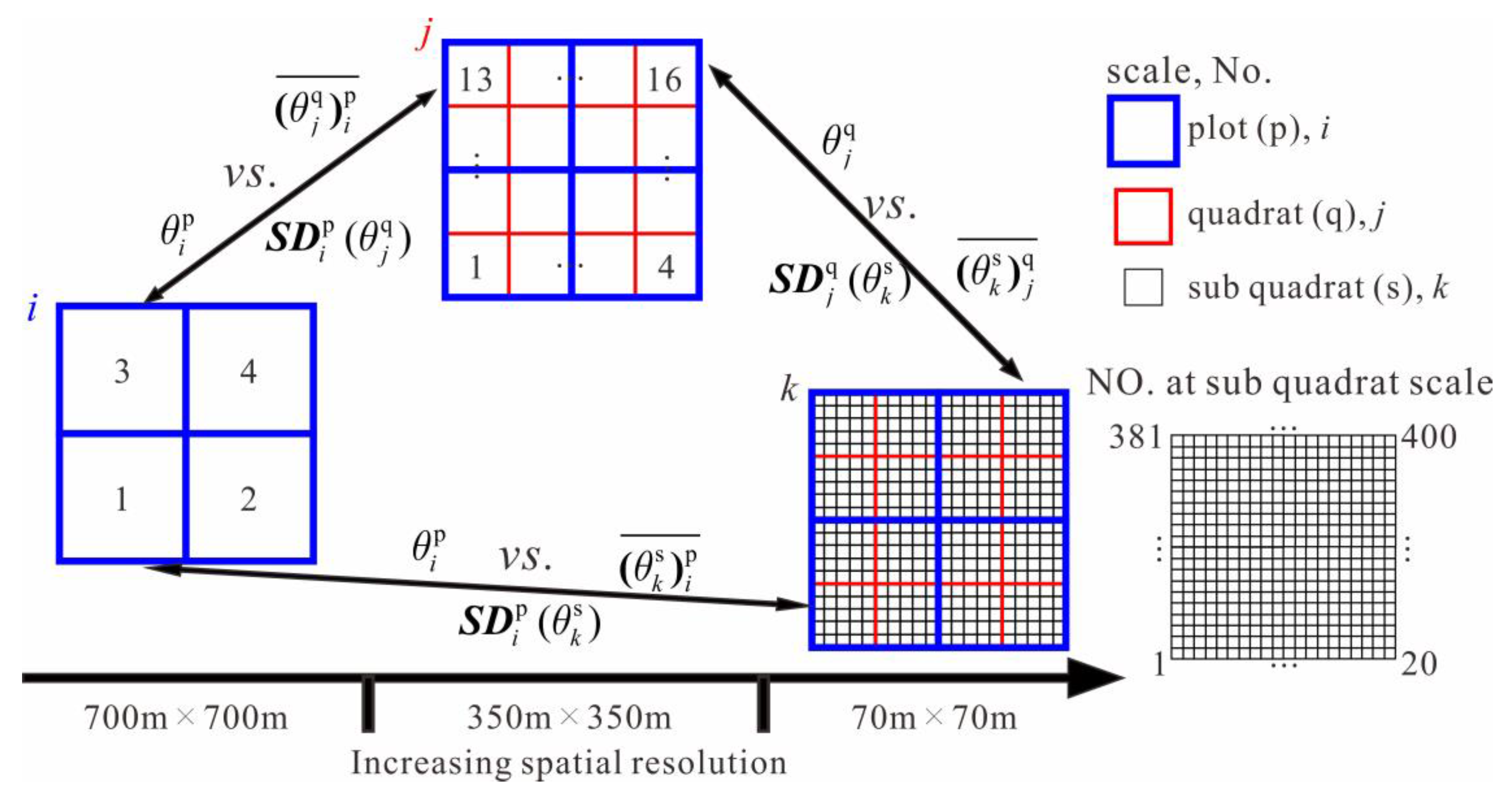
The mismatch between the observational scales of satellite RS and in situ sensor measurements for soil moisture stems from the differences in the fractal dimensions [60,65]. The ISMO data are zero-dimensional data, and the RS data are two-dimensional data. Therefore, an upscaling method for ISMO to RS footprints can remedy the differences caused by different observational scales. 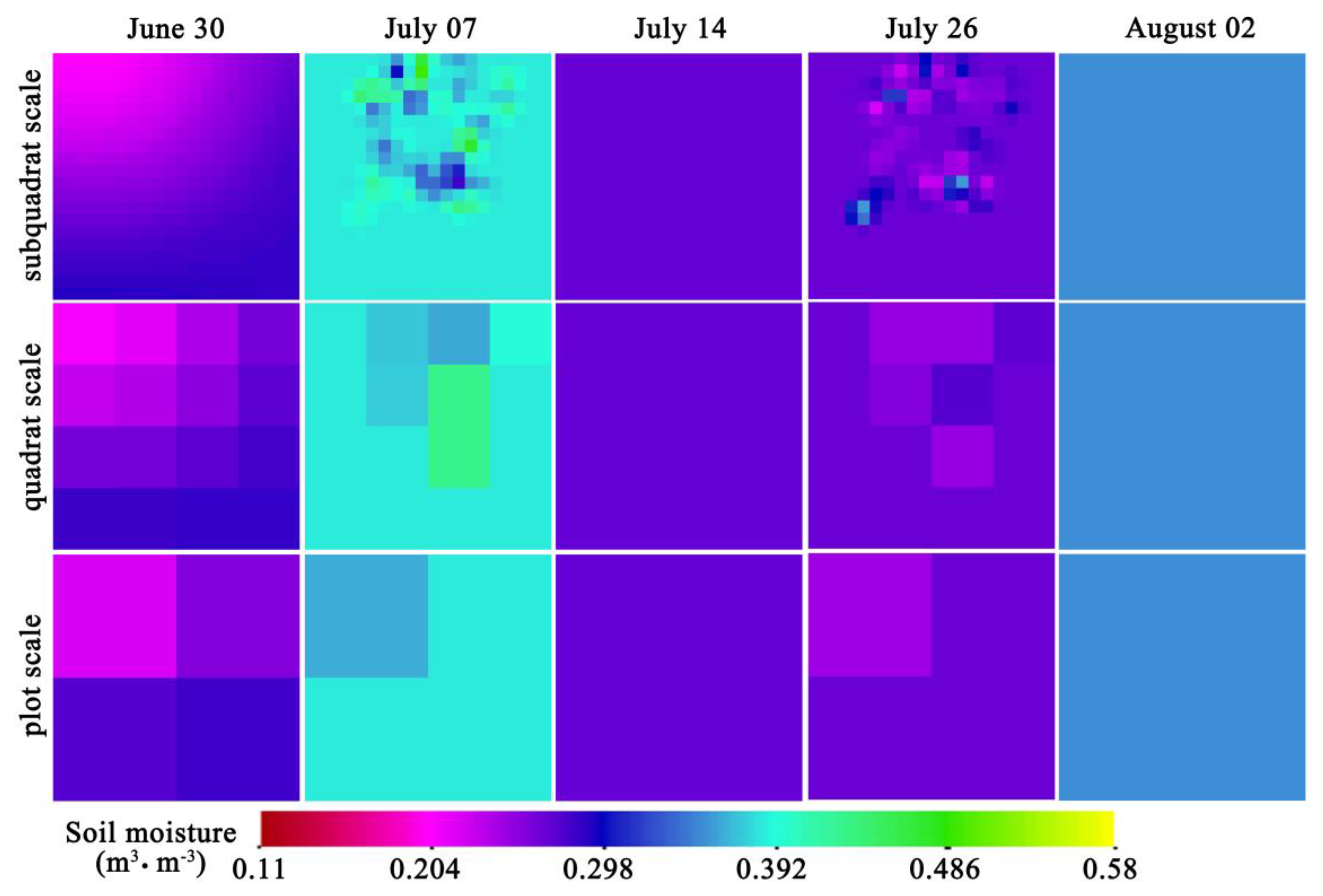Observational scales are believed to consist of three different scales: support (resolution or grain in landscape ecology), spacing (lag), and extent [60]. In reality, soil moisture products are characterized by diverse resolutions, and the various resolutions mean that there are multiple support scales and target scales in the upscaling processes for ISMO. Thus, a spatial scale series (subquadrat, quadrat, and plot) was established as the target scale for the ISMO upscaling processes and the USME at the scale series based on BK, OK, and SA were obtained. The scale series shows an even hierarchy nesting relation (another expression for multiscale [50,66,67]), and the hierarchical idea provides a method to represent or quantify the multiresolution characteristics of RS data and a basis for analyzing multiscale issues that arise in the ISMO upscaling process. However, the actual RS soil moisture products with diverse resolution may not show such a nested relation, and it should be noted in future research.

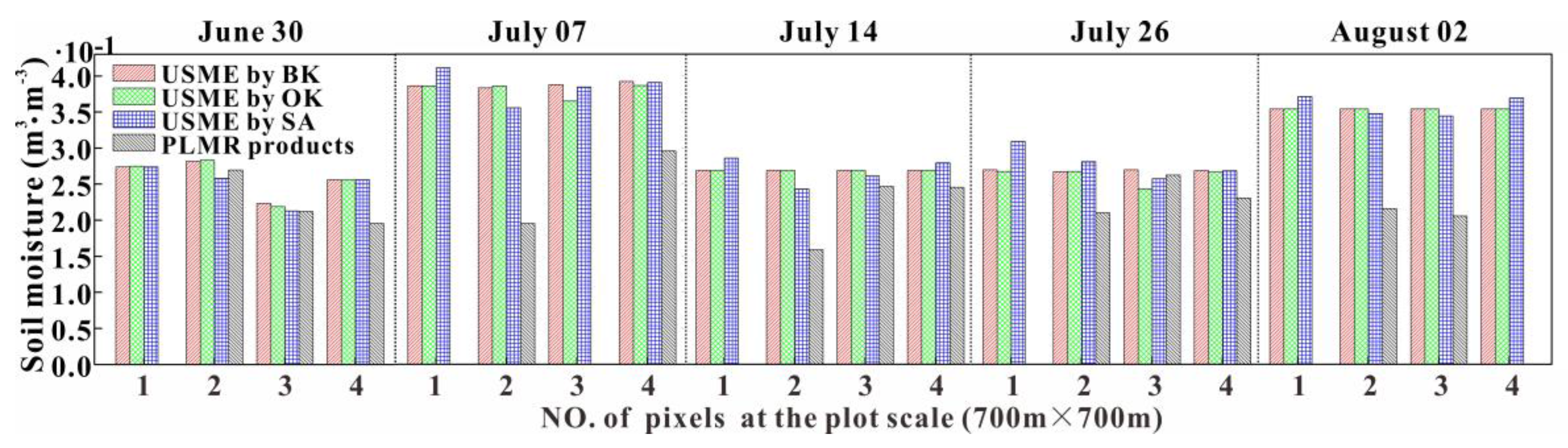
Statistical index analysis (average value and standard deviation), spatial trend surface analysis, and comparison analysis against RS data were conducted to reveal the scale effects in the hierarchical geographical data structures. These scale effects were explained from the perspective of spatial heterogeneity revealed by semivariogram analysis on the original in situ point data. According to the results, when the target scale is shorter than the range of the semivariogram (phenomenon scale) of ISMO, or when the original in situ soil moisture data are spatially homogeneous within the RS observational scale, BK, OK, and SA could be selected as the upscaling methods because the differences between the RS data and the estimations upscaled by those methods are relatively slight, and the kriging methods are not worse than the SA method.

RS soil moisture data contains large uncertainties, and several studies have been conducted to validate satellite-based soil moisture products by upscaling in situ measurements using a modified method [20,22,27]. In some works, the comparisons of upscaled data against RS data differ in the different spatial heterogeneity of in situ data, and the reliability of the validation is sensitive to the spatial variation of the input observation data [18,27,28]. This also adds reliability to the conjectures in our paper. Thus, employing a modified kriging method to verify the accuracy of satellite-based soil moisture products may not be universally applicable. This applicability would be influenced by the spatial structures of the ISMO and the parameters of the kriging model, both of which contain large uncertainties. If we obtain multiresolution RS data in future research, this conclusion would be enhanced and perfected.

According to our results, when the target scale is shorter than the range of the semivariogram of ISMO, the USME upscaled by BK presents the following clear characteristics compared with those by OK and SA: the actual upscaled estimation of each LS pixel is relatively close to the arithmetic average of those of the SS pixels within each LS pixel; the multiscale estimations maintain consistent scale effects and similar global trend surfaces throughout the upscaling process (

Table 7. Comparison of scale effects among scale series according to the magnitude of the target scale and the range based on the upscaled soil moisture estimations (USME) of SoilNET.

Block Kriging	Target Scale < Range	Target Scale > Range
USME vs RS	Stable difference	Unstable difference
Statistical characteristics	Pixel estimations at a larger scale are similar to the averaged value of those at the subscale.	Pixel estimations at a larger scale are different from the averaged value of those at the subscale.
	Analogous scale effects among different zones.	Disparate scale effects among different zones.
Spatial characteristics	Similar global trend surface at a series of scales as indicated by an F test.	-

). Thus, from the standpoint of upscaling ISMO to multiscale pixel estimations covering the RS footprint with only one upscaling method, the USME by BK at the scale series are more statistically comparable and more spatially stable, and are more appropriate for upscaling ISMO. When the target scale is larger than the range of the selected semivariogram of ISMO, the statistical comparability and the spatial stability of the USME by BK are lost and the variability of the USME by BK and OK continually declines with decreasing spatial resolutions. Moreover, when original in situ soil moisture data has no spatial autocorrelation (range equal to 0), the spatial process can be modelled as a pure nugget effect, the weights in Equation (2) all become 1/n, and the estimation procedure becomes an average of all ISMO [23]. Hence, the USME by kriging are constant values at each scale. In the latter two conditions, a kriging method with the selected semivariogram model should not be used to upscale ISMO, but the SA method based on the sample points within each pixel is more suitable.

Moreover, many previous studies have applied variogram modeling and the characteristic length (or range) to evaluate the spatial variability at different observational scales and its impact (change in support) [43,68,69]. However, in our research, to validate the conjectures shown in Table 7, the SoilNET and WaterNET soil moisture data from the HiWATER project [17] within the study area were merged, and these merged data on 30 June (range: 1325.13 m), 7 July (range: 121.1 m), and 26 July (range: 128.7 m) were utilized to repeat the methods mentioned above. The results of the $\mathit{R}\mathit{M}\mathit{S}\mathit{E}({\theta }^{\mathrm{P}},{\theta }^{\mathrm{RS}})$ and $\mathit{R}\mathit{M}\mathit{S}\mathit{E}({\theta }^{\mathrm{LS}},{({\overline{\theta }}^{\mathrm{SS}})}^{\mathrm{LS}})$ for the merged data on 30 June, 7 July, and 26 July are shown in

Table 8. Comparison of upscaled soil moisture estimations at the plot scale (p) against remote sensing (RS) data with RMSE; comparison of the upscaled soil moisture estimations of the larger scale pixels and the averaged value of the smaller scale pixel estimations within each larger scale pixel with RMSE for SoilNET and WaterNET merged data. Units are (m³·m⁻³).

	Block Kriging			Ordinary Kriging
	30 June	7 July	26 July	30 June	7 July	26 July
$\mathit{RMSE}({\theta }^{\mathrm{P}},{\theta }^{\mathrm{RS}})$	2.76·10−2	1.32·10−1	3.00·10−2	1.72·10−3	1.38·10−2	1.74·10−2
$\mathit{RMSE}({\theta }^{\mathrm{p}},{({\overline{\theta }}^{\mathrm{q}})}^{\mathrm{p}})$	0	3.59·10−3	4.10·10−3	1.72·10−3	1.33·10−2	1.74·10−2
$\mathit{RMSE}({\theta }^{\mathrm{p}},{({\overline{\theta }}^{\mathrm{s}})}^{\mathrm{p}})$	0	4.12·10−3	4.08·10−3	4.26·10−4	1.80·10−2	1.07·10−2
$\mathit{RMSE}({\theta }^{\mathrm{q}},{({\overline{\theta }}^{\mathrm{s}})}^{\mathrm{q}})$	0	1.76·10−3	9.19·10−4	1.72·10−3	1.38·10−2	1.74·10−2

and the results of ${\mathit{SD}}^{\mathrm{LS}}({\theta }^{\mathrm{SS}})$ are shown in Figure 11. The linear trend surface analyses for those data on 30 June are shown in

Table 9. The linear trend surface analysis for SoilNET and WaterNET merged data on 30 June. (F_0.05: F value with a significance level of 0.05).

Method	Scale	b0	b1	b2	F Ratio	F0.05
Block Kriging	Sub Quadrat	210.414	1.58·10−5	−5.11·10−5	3113.467	3.018
	Quadrat	211.698	1.60·10−5	−5.15·10−5	115.135	3.806
	Plot	215.968	1.65·10−5	−5.25·10−5	11.639	199.5
Ordinary Kriging	Sub Quadrat	210.569	1.59·10−5	−5.12·10−5	3110.593	3.018
	Quadrat	215.686	1.64·10−5	−5.24·10−5	112.469	3.806
	Plot	233.447	1.82·10−5	−5.68·10−5	10.524	199.5

. As shown in these charts, the USME for these data with kriging on 30 June, 7 July, and 26 July demonstrate these conjectures.

Previous studies have calculated soil moisture variance or standard deviation (STD) at different scales and noted that soil moisture variability decreased with increasing support but increased with extent scale [3,40,53,69]. However, averaged values and STD are insufficient for multiscale modeling of USME. Some landscape ecologists and geographers have built multiscale models on hierarchical data. These researchers believe that the value of a spatial unit (e.g., a pixel) at the lowest level can be determined by the overall mean, the effect of the lowest level, the effect of the median level, and the effect of the highest level [66,67]. These models may be beneficial for formulizing multiscale relations and should be studied. Hence, in this paper, a modified STD was calculated based on hierarchical nesting pixels to benefit the analysis of the scale effects.

The kriging method proved to be suitable for the field level through the cross-validation in this study. However, predicting the data over a larger area using sparse samples in an incomparable small region still needs to be studied. The foregoing analysis methods were applied to the kriging upscaling method and simple averaging upscaling method, and not to the other two common upscaling methods [22]. Whether scale dependence or scale effects exist in multiscale estimations using those surplus two methods and whether they are caused by the spatial structure of the soil moisture data are ongoing topics of research. Moreover, we notice that the choice of theoretical semivariogram model is important for a semivariogram analysis, and, in our research, different spatial processes of soil moisture occurred on different acquisition dates [33]. We cannot stick to a unique theoretical semivariogram model. A different theoretical semivariogram brings about a different empirical semivariogram with different parameters [35,46,58]. The statistical ways or empirical ways for choosing an applicable theoretical semivariogram are not always practical. The simple ways by cross-validation and sensitivity analysis are only helpful in selecting a relatively more applicable model, but cannot determine a unique ideal model. Hence, spatial heterogeneity of the same dataset differs with different selected semivariogram models, which is critical in the kriging method. This is the main reason for uncertainties, including scale effects, in upscaling IMSO to pixel estimations with kriging. Besides this, we did not analyze the relation between any of the parameters of the semivariogram other than the range and their scale effects in the multiscale ISMO upscaling processes, both of which need to be further discussed.

6. Conclusions

In the comprehensive usage of ISMO and RS soil moisture data at the field level, the upscaling of in situ soil moisture observations to multiscale pixel estimations using kriging is an essential approach and is faced with many uncertainties brought upon by scale issues and spatial heterogeneity, which was confirmed by the results of our research.

This work suggests using a semivariogram analysis, which captures the spatial correlation patterns of the original in situ point data and is crucial and effective for explaining these uncertainties and predicting scaling behaviors. The size relations between the range of the semivariogram and the target scales indicate the relation between the phenomenon scale and the observational scale of the studied data and could affect those uncertainties. When the phenomenon scale is larger than the target scales, the differences between the upscaled estimations and the target scale data are relatively slight and estimations by BK would show some relatively apparent characteristics, more so than those by OK. The direct pixel estimation by BK of each LS pixel is relatively close to the mean of those estimations of the SS pixels within each LS pixel, and the multiscale estimations by BK maintain consistent scale effects and similar global trend surfaces throughout the upscaling process.

The results of this research provide a useful reference for studies that need to use satellite-based soil moisture products and ground-based observations at the field level. The most important and first thing to consider is the size relation between the target scale of the satellite-based soil moisture products and the range of the candidate semivariogram on the in situ observations. Upscaled pixel estimations based on in situ observations by kriging with a range shorter than the target scale are not recommended to directly calibrate satellite-based products at the field level. Revised kriging with an improved semivariogram model or SA method may be the better choices.

References

1. Dingman, S.L. Physical Hydrology, 3nd ed.; Waveland Press: Long Grove, IL, USA, 2015; p. 68. [Google Scholar]
2. Yan, S.; Jiang, L.; Chai, L.; Yang, J.; Kou, X. Calibration of the L-MEB model for croplands in HiWATER using PLMR observation. Remote Sens. 2015, 7, 10878–10897. [Google Scholar] [CrossRef]
3. Famiglietti, J.S.; Wood, E.F. Multiscale modeling of spatially variable water and energy balance processes. Water Resour. Res. 1994, 30, 3061–3078. [Google Scholar] [CrossRef]
4. Qiu, J.; Crow, W.T.; Mo, X.; Liu, S. Impact of temporal autocorrelation mismatch on the assimilation of satellite-derived surface soil moisture retrievals. IEEE J. Sel. Top. Appl. Earth Obs. Remote Sens. 2014, 7, 3534–3542. [Google Scholar] [CrossRef]
5. Jasper, K.; Calanca, P.; Fuhrer, J. Changes in summertime soil water patterns in complex terrain due to climatic change. J. Hydrol. 2006, 327, 550–563. [Google Scholar] [CrossRef]
6. Schroder, J.H. Soil Moisture-Based Drip Irrigation for Efficicent Use of Water and Nutrients and Sustainability of Vegetables Cropped on Coarse Soils. Mater’s Dissertation, University of Florida, Gainesville, FL, USA, 2006. [Google Scholar]
7. Wagner, W.; Naeimi, V.; Scipal, K.; Jeu, R.D.; Martínez-Fernández, J. Soil moisture from operational meteorological satellites. Hydrogeol. J. 2007, 15, 121–131. [Google Scholar] [CrossRef]
8. Brocca, L.; Hasenauer, S.; Lacava, T.; Melone, F.; Moramarco, T.; Wagner, W.; Dorigo, W.; Matgen, P.; Martínez-Fernández, J.; Llorens, P.; et al. Soil moisture estimation through ASCAT and AMSR-E sensors: An intercomparison and validation study across Europe. Remote Sens. Environ. 2011, 115, 3390–3408. [Google Scholar] [CrossRef]
9. Panciera, R.; Walker, J.P.; Jackson, T.J.; Gray, D.A.; Tanase, M.; Ryu, D.; Monerris, A.; HeathYardley; Rüdiger, C.; Wu, X.; et al. The Soil Moisture Active Passive Experiments (SMAPEx): Toward soil moisture retrieval from the SMAP mission. IEEE Trans. Geosci. Remote Sens. 2014, 52, 490–507. [Google Scholar] [CrossRef]
10. Pierdicca, N.; Fascetti, F.; Pulvirenti, L.; Crapolicchio, R.; Muñoz-Sabater, J. Analysis of ASCAT, SMOS, in-situ and land model soil moisture as a regionalized variable over Europe and North Africa. Remote Sens. Environ. 2015, 170, 280–289. [Google Scholar] [CrossRef]
11. AMSR-E Overview. Available online: http://www.ospo.noaa.gov/Products/land/smops/sensors-AMSRE.html (accessed on 7 August 2016).
12. ASCAT Products Overview. Available online: http://oiswww.eumetsat.org/WEBOPS/eps-pg/ASCAT/ASCAT-PG-4ProdOverview.htm#TOC4422 (accessed on 11 August 2011).
13. SMAP: Specifications. Available online: https://smap.jpl.nasa.gov/observatory/specifications.html (accessed on 7 August 2016).
14. Merlin, O.; Al Bitar, A.; Walker, J.P.; Kerr, Y. An improved algorithm for disaggregating microwave-derived soil moisture based on red, near-infrared and thermal-infrared data. Remote Sens. Environ. 2010, 114, 2305–2316. [Google Scholar] [CrossRef] [Green Version]
15. Piles, M.; Camps, A.; Vall-llossera, M.; Corbella, I.; Panciera, R.; Rudiger, C.; Kerr, Y.H.; Walker, J. Downscaling SMOS-derived soil moisture using MODIS visible/infrared data. IEEE Trans. Geosci. Remote Sens. 2011, 49, 3156–3166. [Google Scholar] [CrossRef]
16. Bogena, H.R.; Herbst, M.; Huisman, J.A.; Rosenbaum, U.; Weuthen, A.; Vereecken, H. Potential of wireless sensor networks for measuring soil water content variability. Vadose Zone J. 2010, 9, 1002–1013. [Google Scholar] [CrossRef]
17. Li, X.; Cheng, G.; Liu, S.; Xiao, Q.; Ma, M.; Jin, R.; Che, T.; Liu, Q.; Wang, W.; Qi, Y.; et al. Heihe Watershed Allied Telemetry Experimental Research (HiWATER): Scientific objectives and experimental design. Bull. Am. Meteorol. Soc. 2013, 94, 1145–1160. [Google Scholar] [CrossRef]
18. Kang, J.; Jin, R.; Li, X. Regression kriging-based upscaling of soil moisture measurements from a wireless sensor network and multiresource remote sensing information over heterogeneous cropland. IEEE Geosci. Remote Sens. Lett. 2015, 12, 92–96. [Google Scholar] [CrossRef]
19. Kang, J.; Jin, R.; Li, X.; Ma, C.; Qin, J.; Zhang, Y. High spatio-temporal resolution mapping of soil moisture by integrating wireless sensor network observations and MODIS apparent thermal inertia in the Babao River Basin, China. Remote Sens. Environ. 2017, 191, 232–245. [Google Scholar] [CrossRef]
20. Crow, W.T.; Berg, A.A.; Cosh, M.H.; Loew, A.; Mohanty, B.P.; Panciera, R.; de Rosnay, P.; Ryu, D.; Walker, J.P. Upscaling sparse ground-based soil moisture observations for the validation of coarse-resolution satellite soil moisture products. Rev. Geophys. 2012, 50, 3881–3888. [Google Scholar] [CrossRef]
21. Colliander, A.; Jackson, T.J.; Bindlish, R.; Chan, S.; Das, N.; Kim, S.B.; Cosh, M.H.; Dunbar, R.S.; Dang, L.; Pashaian, L.; et al. Validation of SMAP surface soil moisture products with core validation sites. Remote Sens. Environ. 2017, 191, 215–231. [Google Scholar] [CrossRef]
22. Qin, J.; Zhao, L.; Chen, Y.; Yang, K.; Yang, Y.; Chen, Z.; Lu, H. Inter-comparison of spatial upscaling methods for evaluation of satellite-based soil moisture. J. Hydrol. 2015, 523, 170–178. [Google Scholar] [CrossRef]
23. Isaaks, E.H.; Srivastava, R.M. An Introduction to Applied Geostatistics; Oxford University Press: Oxford, NY, USA, 1989; pp. 120, 181, 278–330, 373–375. [Google Scholar]
24. Crow, W.T.; Ryu, D.; Famiglietti, J.S. Upscaling of field-scale soil moisture measurements using distributed land surface modeling. Adv. Water Resour. 2005, 28, 1–14. [Google Scholar] [CrossRef]
25. Mohanty, B.P.; Skaggs, T.H.; Famiglietti, J.S. Analysis and mapping of field-scale soil moisture variability using high-resolution, ground-based data during the Southern Great Plains 1997 (SGP97) Hydrology Experiment. Water Resour. Res. 2000, 36, 1023–1031. [Google Scholar] [CrossRef]
26. Woodley, W.J. Investigating the Upscaling of In Situ Soil Moisture Measurements for Satellite Validation. Mater’s Dissertation, The University of Guelph, Guelph, ON, Canada, 2017. [Google Scholar]
27. Wang, J.; Ge, Y.; Heuvelink, G.B.M.; Zhou, C. Upscaling in situ soil moisture observations to pixel averages with spatio-temporal geostatistics. Remote Sens. 2015, 7, 11372–11388. [Google Scholar] [CrossRef]
28. Lakhankar, T.; Jones, A.S.; Combs, C.L.; Sengupta, M.; Vonder Haar, T.H.; Khanbilvardi, R. Analysis of large scale spatial variability of soil moisture using a geostatistical method. Sensors 2010, 10, 913–932. [Google Scholar] [CrossRef] [PubMed]
29. Johnston, K.; Hoef, J.M.V.; Krivoruchko, K.; Lucas, N. Using ArcGIS Geostatistical Analyst; Esri: Redlands, CA, USA, 2001; p. 216. [Google Scholar]
30. Li, X.; Liu, S.; Xiao, Q.; Ma, M.; Jin, R.; Che, T.; Wang, W.; Hu, X.; Xu, Z.; Wen, J.; et al. A multiscale dataset for understanding complex eco-hydrological processes in a heterogeneous oasis system. Sci. Data 2017, 4, 170083. [Google Scholar] [CrossRef] [PubMed]
31. Jin, R.; Li, D. HiWATER: Dataset of Retrieved Soil Moisture Products Using PLMR Brightness Temperatures in the Middle Reaches of the Heihe River Basin; Cold and Arid Regions Science Data Center: Gansu, China, 2014. [Google Scholar]
32. Kang, J.; Li, X.; Jin, R.; Ge, Y.; Wang, J.; Wang, J. Hybrid optimal design of the eco-hydrological wireless sensor network in the middle reach of the Heihe River Basin, China. Sensors 2014, 14, 19095–19114. [Google Scholar] [CrossRef] [PubMed]
33. Jin, R.; Li, X.; Yan, B.; Li, X.; Luo, W.; Ma, M.; Guo, J.; Kang, J.; Zhu, Z.; Zhao, S. A nested eco-hydrological wireless sensor network for capturing the surface heterogeneity in the midstream area of the Heihe River Basin, China. IEEE Geosci. Remote Sens. Lett. 2014, 11, 2015–2019. [Google Scholar] [CrossRef]
34. Che, T.; Li, X.; Gao, Y.; Walker, J. HiWATER: Dataset of Airborne Microwave Radiometers (L Bands) Mission in the Middle Reaches of the Heihe River Basin on Jun. 30, 2012; Heihe Plan Science Data Center: Gansu, China, 2013. [Google Scholar]
35. Webster, R.; Oliver, M.A. Geostatistics for Environmental Scientists, 2nd ed.; Wiley: Chichester, UK, 2007; pp. 17–18, 40–42, 58, 70, 110, 113. [Google Scholar]
36. Publishing, S.; Publishing, P.S. SAS Procedures Guide: Version 6, 3nd ed.; SAS Institute Inc.: Cary, NC, USA, 1989. [Google Scholar]
37. Kitanidis, P.K. Introduction to Geostatistic Application to Hydrogeology; Cambridge University Press: Cambridge, UK, 1997. [Google Scholar]
38. Kerry, R.; Oliver, M.A. Determining the effect of asymmetric data on the variogram. II. Outliers. Comput. Geosci. 2007, 33, 1233–1260. [Google Scholar] [CrossRef]
39. Gharechelou, S.; Tateishi, R.; Sharma, R.C.; Johnson, B.A. Soil Moisture Mapping in an Arid Area Using a Land Unit Area (LUA) Sampling Approach and Geostatistical Interpolation Techniques. ISPRS Int. J. Geo-Inf. 2016, 5, 35. [Google Scholar] [CrossRef]
40. Ryu, D.; Famiglietti, J.S. Multi-scale spatial correlation and scaling behavior of surface soil moisture. Geophys. Res. Lett. 2006, 33, L08404. [Google Scholar] [CrossRef]
41. Matheron, G. Principles of geostatistics. Econ. Geol. 1963, 58, 1246–1266. [Google Scholar] [CrossRef]
42. Wu, H.; Li, Z. Scale issues in remote sensing: A review on analysis, processing and modeling. Sensors 2009, 9, 1768–1793. [Google Scholar] [CrossRef] [PubMed]
43. Western, A.W.; Blöschl, G.; Grayson, R.B. Geostatistical characterisation of soil moisture patterns in the Tarrawarra catchment. J. Hydrol. 1998, 205, 20–37. [Google Scholar] [CrossRef]
44. Pebesma, E.J. The gstat package. Comput. Geosci. 2004, 30, 683–691. [Google Scholar] [CrossRef]
45. Beveridge, D.; St-Hilaire, A.; Ouarda, T.B.M.J.; Khalil, B.; Conly, F.M.; Wassenaar, L.I.; Ritson-Bennett, E. A geostatistical approach to optimize water quality monitoring networks in large lakes: Application to Lake Winnipeg. J. Great Lakes Res. 2012, 38, 174–182. [Google Scholar] [CrossRef]
46. Kresic, N.; Mikszewski, A. Hydrogeological Conceptual Site Models: Data Analysis and Visualization; CRC press: Boca Raton, FL, USA, 2012; p. 283. [Google Scholar]
47. Rao, S.S. Engineering Optimization: Theory and Practice, 4th ed.; John Wiley and Sons: Hoboken, NJ, USA, 2009. [Google Scholar]
48. Esri, Inc. How Semivariogram Sensitivity Works. ArcGIS 10.4 Help Library. Available online: https://desktop.arcgis.com/en/arcmap/10.4/extensions/geostatistical-analyst/how-semivariogram-sensitivity-works.htm (accessed on 7 December 2016).
49. Wilson, A.M.; Silander, J.A.; Gelfand, A.; Glenn, J.H. Scaling up: Linking field data and remote sensing with a hierarchical model. Int. J. Geogr. Inf. Sci. 2011, 25, 509–521. [Google Scholar] [CrossRef]
50. Panagos, P.; Liedekerke, M.V.; Montanarella, L. Multi-scale European Soil Information System (MEUSIS): A multi-scale method to derive soil indicators. Comput. Geosci. 2011, 15, 463–475. [Google Scholar] [CrossRef]
51. Lloyd, C.D. Exploring Spatial Scale in Geography; John Wiley and Sons: Chichester, UK, 2014. [Google Scholar]
52. Cosh, M.H.; Jacksona, T.J.; Bindlishb, R.; Pruegerc, J.H. Watershed scale temporal and spatial stability of soil moisture and its role in validating satellite estimates. Remote Sens. Environ. 2004, 92, 427–435. [Google Scholar] [CrossRef]
53. Famiglietti, J.S.; Ryu, D.; Berg, A.A.; Rodell, M.; Jackson, T.J. Field observations of soil moisture variability across scales. Water Resour. Res. 2008, 44, W01423. [Google Scholar] [CrossRef]
54. Clark, J.S.; Gelfand, A.E. A future for models and data in environmental science. Trends Ecol. Evol. 2006, 21, 375–380. [Google Scholar] [CrossRef] [PubMed]
55. Parsley, A.J. Application of autocorrelation criteria to the analysis of mapped geologic data from the coal measures of central England. Math. Geol. 1971, 3, 281–295. [Google Scholar] [CrossRef]
56. Unwin, D.J. An Introduction to Trend Surface Analysis; Geo Abstracts: Norwich, UK, 1978; Volume 5. [Google Scholar]
57. Cliff, A.D.; Kelly, F.P. Regional taxonomy using trend-surface coefficients and invariants. Environ. Plan. A 1977, 9, 945–955. [Google Scholar] [CrossRef]
58. McBratney, A.B.; Webster, R. Choosing functions for semi-variograms of soil properties and fitting them to sampling estimates. J. Soil Sci. 1986, 37, 617–639. [Google Scholar] [CrossRef]
59. Zhang, X.; Jiang, L.; Qiu, X.; Qiu, J.; Wang, J.; Zhu, Y. An improved method of delineating rectangular management zones using a semivariogram-based technique. Comput. Electron. Agric. 2016, 121, 74–83. [Google Scholar] [CrossRef]
60. Blöschl, G.; Sivapalan, M. Scale issues in hydrological modelling: A review. Hydrol. Processes 1995, 9, 251–290. [Google Scholar] [CrossRef]
61. Montello, D.R. Scale in geography. Int. Encycl. Soc. Behav. Sci. 2001, 4, 13501–13504. [Google Scholar]
62. Wu, J. Effects of changing scale on landscape pattern analysis: Scaling relations. Landsc. Ecol. 2004, 19, 125–138. [Google Scholar] [CrossRef]
63. Perveen, S.; James, L.A. Multiscale Effects on Spatial Variability Metrics in Global Water Resources Data. Water Resour. Manag. 2010, 24, 1903–1924. [Google Scholar] [CrossRef]
64. Quattrochi, D.A.; Wentz, E.; Lam, N.S.N.; Emerson, C.W. Integrating Scale in Remote Sensing and GIS; Routledge: Oxfordshire, UK, 2017. [Google Scholar]
65. Lam, N.S.N.; Quattrochi, D.A. On the issues of scale, resolution, and fractal analysis in the mapping sciences. Prof. Geogr. 1992, 44, 88–98. [Google Scholar] [CrossRef]
66. Moellering, H.; Tobler, W. Geographical variances. Geogr. Anal. 2010, 4, 34–50. [Google Scholar] [CrossRef]
67. Wu, J.; Jelinski, D.E.; Luck, M.; Tueller, P.T. Multiscale analysis of landscape heterogeneity scale variance and pattern metrics. Geogr. Inf. Sci. 2000, 6, 6–19. [Google Scholar] [CrossRef] [PubMed]
68. Artan, G.A.; Neale, C.M.U.; Tarboton, D.G. Characteristic length scale of input data in distributed models: Implications for modeling grid size. J. Hydrol. 2000, 227, 128–139. [Google Scholar] [CrossRef]
69. Western, A.W.; Blöschl, G. On the spatial scaling of soil moisture. J. Hydrol. 1999, 217, 203–224. [Google Scholar] [CrossRef]
Figure 1. The map of study area with the locations of SoilNET and polarimetric L-band multibeam radiometer (PLMR) products (c). The study area is in Heihe River Basin (e), in the north of China (d). The photos were taken in the Yingke (a) and Daman (b) irrigation districts and are reprinted from Farmland Ecosystem observation site, http://www.chinaflux.org/.
Ijgi 07 00033 g001
Figure 2. SoilNET soil moisture (SM) except deleted outliers and PLMR products (white color means no data).
Ijgi 07 00033 g002
Figure 3. The technical flow chart for methodologies in this paper.
Ijgi 07 00033 g003
Figure 4. A directed acyclic graph [54] is used to illustrate the hierarchical model structure and to analyze the statistical characteristics of the upscaled soil moisture estimations (USME) using block kriging, ordinary kriging, and simple averaging. θ ( m 3 · m 3 ) = USME; i : number of pixels at the plot scale (p); j : number of pixels at the quadrat scale (q); k : number of pixels at the subquadrat scale (s); θ ¯ : arithmetic mean of θ ; S D : modified standard deviation. The double-sided arrows are used to join the scales that are compared with each other.
Ijgi 07 00033 g004
Figure 5. Semivariograms of in situ soil moisture observations: (a) 30 June data, using a Gaussian model; (b) 7 July data, using a Spherical model; (c) 14 July data, using a pure nugget effect model; (d) 26 July, using a Spherical model; and (e) 2 August, using a pure nugget effect model. (a) 0.002·Nugget + 0.002·Gaussian(1179.7); (b) 0.001·Nugget + 0.005·Spherical(139.0); (c) 0.002·Nugget; (d) 0.005·Nugget + 0.034·Spherical(132.0); (e) 0.021·Nugget.
Ijgi 07 00033 g005aIjgi 07 00033 g005b
Figure 6. Upscaled soil moisture estimations at the scale series by block kriging on five acquisition days.
Ijgi 07 00033 g006
Figure 7. Upscaled soil moisture estimations at the scale series by ordinary kriging on five acquisition days.
Ijgi 07 00033 g007
Figure 8. Upscaled soil moisture estimations at the scale series by simple averaging on five acquisition days.
Ijgi 07 00033 g008
Figure 9. Box plots of the standard deviations based on block kriging (a), ordinary kriging (b), and simple averaging (c) estimations in the smaller scale (SS) pixels within each pixel at the larger scale (LS) on five acquisition days from 30 June to 2 August: SD LS ( θ SS ) (m3·m−3). The box boundaries indicate the 25th and 75th percentiles, the whiskers below and above the box indicate the min and max, the line within the box marks the median, and the point in the box indicates the mean.
Ijgi 07 00033 g009
Figure 10. PLMR soil moisture products and upscaled soil moisture estimations (USME) (m3 × m−3) at the scale series by block kriging (BK), ordinary kriging (OK), and simple averaging (SA) on five acquisition days.
Ijgi 07 00033 g010
Figure 11. Box plots of standard deviations (m3·m−3) based on upscaled estimations by block kriging (a), ordinary kriging (b), and simple averaging (c) of the smaller scale pixel within each larger scale pixel on 30 June, 7 July, and 26 July.
Ijgi 07 00033 g011