DASSCAN: A Density and Adjacency Expansion-Based Spatial Structural Community Detection Algorithm for Networks

1
School of Resource and Environmental Sciences, Wuhan University, Wuhan 430079, China
2
Key Laboratory of Geographic Information System, Ministry of Education, Wuhan University, Wuhan 430079, China
3
Collaborative Innovation Center for Geospatial Information Technology, Wuhan University, Wuhan 430079, China
*
Author to whom correspondence should be addressed.
ISPRS Int. J. Geo-Inf. 2018, 7(4), 159; https://0-doi-org.brum.beds.ac.uk/10.3390/ijgi7040159
Submission received: 12 March 2018
/
Revised: 15 April 2018
/
Accepted: 19 April 2018
/
Published: 21 April 2018
Abstract
:Existing spatial community detection algorithms are usually modularity based. Motivated by different applications, these algorithms build appropriate spatial null models to describe spatial effects on the connection of nodes. Then, by choosing certain modularity maximizing strategies, they try to find interesting community structures hidden behind the null models. In this paper, a novel structural similarity-based spatial network community is defined, which is based on the shared neighbors of nodes. In addition, there are two other special node roles defined: the spatial hub and outlier. Then, a density and adjacency expansion-based spatial structural community detection algorithm for networks (DASSCAN) is proposed for mining these communities, hubs and outliers. DASSCAN uses structural similarity to measure the relationship between nodes, and then, structurally similar and spatially adjacent nodes are merged into communities using a density-based clustering method and spatial adjacency expansion strategy. Comparative experiments on two kinds of Chinese train line networks clarified the accuracy and efficiency of DASSCAN in finding the spatial structural communities, spatial hubs and outliers. The communities found can be used to uncover more interesting spatial structural patterns, and the hubs and outliers are more accurate and have more valuable meanings.
1. Introduction and Motivations
Spatial networks are networks in which nodes are in a metric-equipped space. For most practical applications, this is a two-dimensional space and the metric is usually the Euclidean distance [1]. Spatial networks commonly exist in our daily lives. Many transportation and infrastructure networks, such as road and street networks, power grids, and communication networks, are constructed in space. Some online location-based service networks, such as Twitter, Facebook and Foursquare, also have geographical attributes within them.
Different from the small world and free scale properties, a community is another basic feature of a complex network [2]. A community is a set of nodes that have more connections among themselves than with the rest of nodes. The research on community detection in complex networks is of fundamental importance. It has both theoretical significance and practical applications in terms of analyzing network topology, comprehending network function, unfolding network patterns and forecasting network activities. Community detection is also an important and fundamental topic in spatial network studies. Community detection can be used to discover interesting spatial patterns and help with understanding the spatial structure hidden in networks. In addition, this method has been used in many areas, such as finding human movement patterns or local pockets of bicycle sharing systems in inner cities [3,4], detecting spatial interaction communities from inner or intra cities [5,6], identifying spatial clusters and partitions of transportation networks [7,8,9,10,11], and discovering global and local structures of research and development cooperation in Europe [12].
The existence of geospatial property and the various spatial relations in spatial network make it different from traditional network. The probability of a link between two nodes in a spatial network will decrease with distance, and will be affected by its nearby nodes. This leads to community detection in spatial networks being more difficult to obtain than in traditional networks. Researchers have proposed several methods that integrate spatial constraints (e.g., spatial contiguity and geographic distance) into the spatial network’s community detection process. These solutions can be classified into four categories:
(1) Ignore the geographic constraint, and directly use the classical community detection algorithms [7,12] or graph partition algorithms [9,10,11] in traditional complex network areas to discover topological structures that exist in the spatial network. In fact, spatial nodes near one another are more likely to be connected than those far apart. Therefore, the spatial patterns of these communities often simply exhibit regional properties, which obviously exist in spatial networks.
(2) Add a spatial contiguity constraint into the hierarchical clustering-based methods [13,14]. First, the agglomerative hierarchical clustering approaches are used to construct a spatially contiguous tree by merging the most connected neighborhood clusters. Then, the spatially contiguous tree is partitioned to obtain regional communities while maximizing the within-region modularity. The inner structures of the discovered communities are spatially connected.
(3) Reconstruct the spatial network by adding inverse distance weights to all the edges, and then modify the classical community detection algorithm to detect geo-communities by optimizing a newly defined geo-modularity [8]. The spatial patterns of these communities tend to be more local than the first category of methods above, since the reconstruction process reinforces the distance decay affects among nodes.
(4) Improve the probability model of NG modularity by integrating a distance decay factor into the topological connection and construct a joint probability model to be the expected probability value [15,16,17,18,19,20,21]. Then, modify the classical community detection algorithm to detect communities that eliminate the space effect and to reveal the hidden structural similarities between nodes. The definition of the classical modularity (NG modularity) involves a fraction of within-community edges in the observed network, as well as that number in an equivalent randomized network [22,23]. This equivalent randomized network is called the null model, which serves as a reference. Researchers argue that the null model in the original definition of modularity is unrealistically mixed, since it does not characterize some features of the observed spatial network (e.g., geographic factors). Thus, it fails to be a good representation of real-world networks. In addition, by constructing various spatial null modularity models (e.g., gravity model [15,21], radiation model [20], and exponential decay model [16,18,19]), the community results will discover other interesting factors of the spatial network. For example, Expert et al. [15] proposed a modified function of modularity-based on connective probability at different distances. These researchers tested their new method with mobile phone data and uncovered a linguistic network partition of the French and Flemish speaking parts of Belgium. This partition was obscured by geographical communities when using the NG modularity.
Most spatial community detection methods mentioned above are modularity-based [1,5,6,7,8,14,15,16,17,18,19,20,24]. The spatial null model is the core point for them. Motivated by different applications, these algorithms build appropriate spatial null models to describe spatial effects on the connection of nodes. Then, by choosing certain modularity maximizing strategies, they try to find interesting community structures hidden behind the null models. Sarzynska et al. [20] investigated the effects of using three null models (radiation null model, gravity null model and the standard NG null model) that incorporate spatial information. They found that the quality of community results with different null models depends strongly on the network and on the parameter settings. Moreover, Good et al. [25] made a careful analysis of modularity and its performance. Several limitations of the modularity-based community detection algorithm were addressed, such as the resolution limit, the extreme degeneracy exhibition of the modularity function, and the limiting behavior of the maximum modularity. Both Sarzynska et al. [20] and Good et al. [25] suggested to use appropriate generative models or combine information from many degenerate solutions for the development of spatial null models.
The graph partition-based methods [9,10,11] and the hierarchical clustering-based methods [4,14] are different from the modularity-based methods. They calculate the similarity or difference based on the attributes of two nodes which have an edge connection. Then, they use spectral clustering or hierarchical clustering algorithms to obtain a partition of the spatial network. The partition corresponds to the community results.
In this paper, a new method for spatial network community detection, known as DASSCAN (a density and adjacency expansion-based spatial structural community detection algorithm for networks), is proposed. DASSCAN uses the shared neighbors’ similarity of nodes as clustering criteria, instead of only using their direct connections. Spatial nodes are grouped into one community when they share many connected neighbors and have an adjacent relationship with each other. Doing so makes sense when considering the detection of communities in spatial networks, such as highway and railway networks. Communities in these spatial networks always expand based on nodes with spatially adjacent relations. The more shared neighbor connections nodes have, the higher the probability they are in the same community.
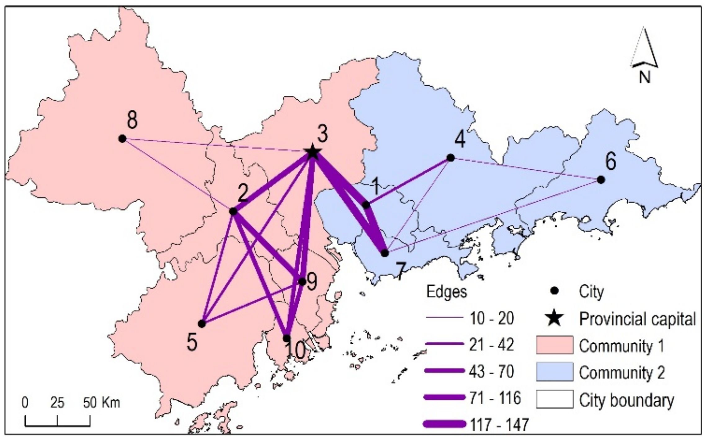
Figure 1 shows the inner city, high-speed train network in the Guangdong Province, China. The edges among nodes are weighted by the number of trains running between two cities. When using one of the popular and efficient modularity-based methods, Louvain [26,27], node 3 belongs to the eastern community because it has very large connections with nearby nodes 1 and 7. However, when setting proper parameters, DASSCAN found that node 3 belongs to the western community. Considering the structural similarity of shared neighbors, node 3 only has two connected nodes (1 and 7) in the eastern community, and it does not share any other neighbors with these two nodes. In contrast, node 3 has connections with all five nodes in the western community, and they share many neighbors among one another. Thus, DASSCAN can identify this spatial structural community, which is different from the community results found by modularity-based method. The new community results reveal the spatial structure of this inner train network very well.
DASSCAN has the following features:
(1) DASSCAN extends the structurally connected cluster [28] into the spatial network domain by combining the spatial contiguity constraint with the node connectivity structures as community detection criteria. Through theoretical analysis and experimental evaluation, we demonstrate that DASSCAN can obtain stable and meaningful community results in spatial networks.
(2) The density-based scanning strategy of DASSCAN can detect communities that maintain contiguity inside, as well as two other community-based node roles in the spatial network, which are spatial hubs and outliers. A spatial hub is a node that has both connections and spatially adjacent relations with more than one community, but the hub does not belong to any of the communities. The spatial hub plays a special role in small world networks [29,30]. In addition, an outlier is a node that has only a weak association with a community. The formal definitions of these roles will be given in the next section.
2. Materials and Methods
This section uses Chinese high-speed train lines to build spatial networks, and then, the DASSCAN algorithm is proposed to detect spatially structural communities, based on the networks.
2.1. Spatial Network Modeling
Chinese high-speed trains are an important spatial network, which connects many rapidly developing cities in China. We chose two kinds of high-speed train lines to model two kinds of spatial networks: the type C intercity high-speed train and type G high-speed train. The train line data were extracted from the official website of the Chinese Railway Customer Service Center [31]. In addition, several pre-processing steps for the two kinds of train lines data are given below:
(1) For each train line, the original train station names are represented by the names of the cities in which they are located. Table 1 lists the two kinds of post-processed train line data. The train numbers in the first column begin with a capital letter, which represents the train line type.
(2) The coordinates of the city’s inner geometry center were used as the geographic location of each node in the spatial network.
(3) The topological adjacency matrix was constructed by checking whether there was a shared boundary between two cities. Since Hainan and Taiwan Provinces are both islands, they do not share boundaries with any others. Thus, train lines in these two provinces are omitted to simplify the data.
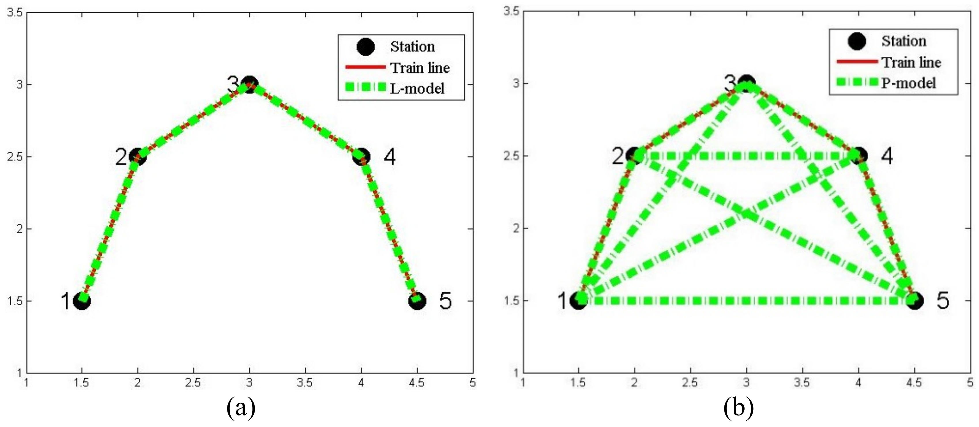
There are two topological models that exist in the transportation network research area: the space L model and space P model [32]. In the space L model, only nearby stations for one train line are considered to have connections. In the space P model, all possible station pairs for the same train line are considered to have connections. Figure 2 shows two networks that are constructed using the two models. As seen in Figure 2, the space P model ignores the topological adjacency between the two nodes and is more focused on the relationship between nodes in the train line. Therefore, the space P model is more suitable for the community detection task. The space P model was chosen to construct the train line networks in this study.
The train line network based on the space P model can be represented by a 0–1 matrix. Each element in the matrix was assigned to 1 when a train passed the two cities. Finally, there were two different spatial networks that contained 167 cities and 3152 train lines. The number of nodes and edges for the two networks are listed in Table 2. In addition, community detection experiments were completed on each of the network.
2.2. DASSCAN Algorithm
In this section, we first formulate the notion of a spatial structural community and two special roles of network nodes: spatial hub and outlier. Then, the DASSCAN algorithm is proposed, which combines the density-based clustering algorithm [33] with a spatial adjacency expansion strategy. The density measure is changed into the structural similarity between nodes in the spatial network. In addition, the community detection process needs to obey the spatial adjacency constraint. DASSCAN can discover spatially connected and well-structured communities, as well as hubs and outliers in spatial networks. Depending on different definitions of structural similarity, DASSCAN can be used for both unweighted and weighted spatial networks. Moreover, similar to the solution in Cazabet et al. [21], by dividing directional networks into two kinds of connections (in-degree connections and out-degree connections), and calculating the two structural similarities, respectively, DASSCAN can also find structural community in directed spatial networks.
Existing spatial network community detection methods only consider the number of edges between nodes or clusters. These direct connections are important in constructing community, but they represent only one aspect of the network structure. The spatial structural community considers the neighborhoods around two connected nodes to also be important. The neighborhood of a node includes all the nodes connected to it by edges. When considering a pair of connected nodes, the combined neighborhood reveals neighbors that are common to both nodes.
For simplification, we only give the definitions of structural similarity based on a simple, undirected and unweighted spatial network. The directed and weighted structural similarity are easy to extend. Let G = {V, E}, which is a spatial network, where V is a set of nodes and E is a set of edges. Each node in G has its own spatial boundary, and AM is the topological adjacency matrix for all nodes. If two nodes have a spatially adjacent relation, the value of the corresponding element in AM equals to 1; otherwise, it equals 0.
A node’s structure can be described by its connected neighborhood. A formal definition of node structure is given as follows.
Definition 1.
Node structure. For a node v ∈ V, the structure of v is defined as a node set composed of v and all of v’s connected neighbors.
There are several functions used to measure the similarity between two vectors (e.g., Cosine and Jaccard). We chose the cosine similarity to calculate the structural similarity between two connected nodes in a spatial network.
Definition 2.
Structural similarity. For a node pair v and u, the structural similarity is defined as follows.
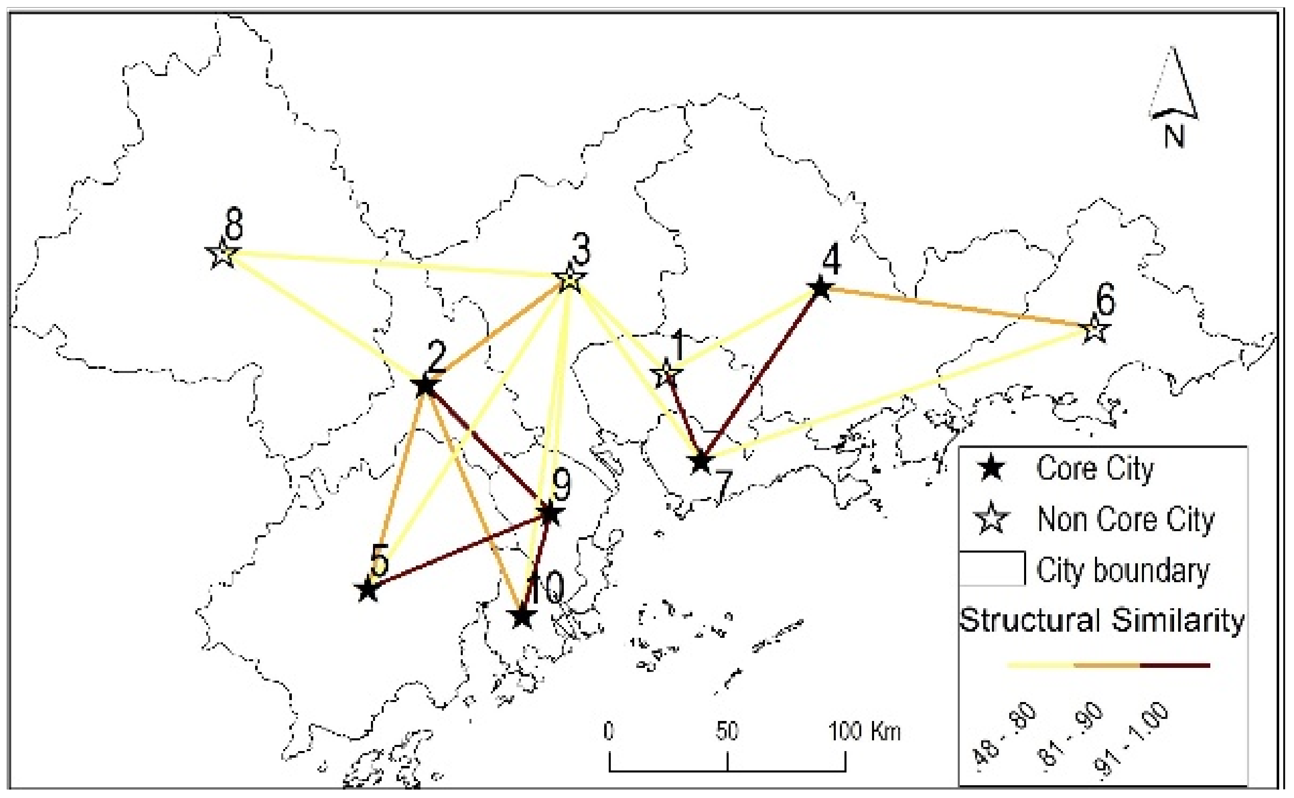
The structural similarities in the sample train network were calculated, as shown in Figure 3. For each edge in the network, there is a corresponding structural similarity value. If the number of connections on each edge has to be considered, then the node structure for each node is a set of neighbor nodes with the connection numbers as their weights. The structural similarity can be calculated by the adjusted cosine similarity:
where Γvu is a set of the shared neighbors of node v and u, is the number of connections between node v and i, and is the average connection of node i.
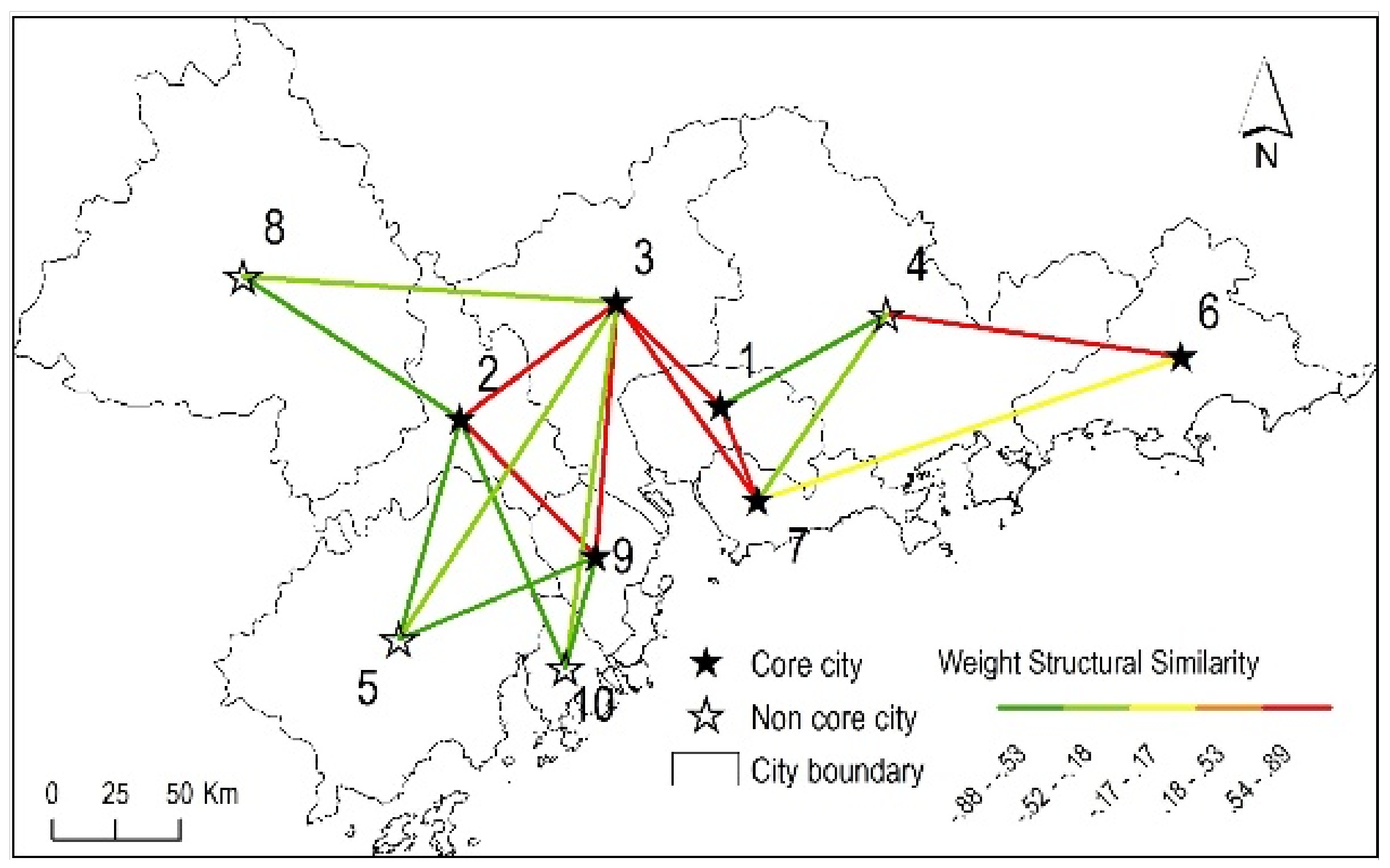
The adjusted cosine similarity is a very efficient item-based neighborhood model in recommender systems. It solves the rating scales problem by subtracting the average connection of the corresponding node from each weighted shared neighbor [34]. It generally provides superior results. For detailed explanations of the adjusted cosine similarity, please refer to [34,35]. Figure 4 draws the weighted structural similarities in the sample train network. As can be seen, the spatial structure is quite different from Figure 3. Figure 3 only reflects the connectional similarity between nodes. Figure 4 emphasizes both connectional similarity (between nodes 4 and 6) and connection intensity (among nodes 1, 2, 3, 7 and 9). Connections from nodes 5 and 10 to nodes 2, 3 and 9 are less than the average connections of the three core nodes, therefore they both obtained negative similarity values to the three core nodes.
To process the density-based clustering for this similarity network, two density parameters, minimum similarity threshold (ε) and minimal number of neighborhoods (μ), are required to find the core node in a spatial network.
Definition 3.
Core node. For a node v, the set of neighbors which have structural similarity greater than ε forms the ε-neighborhood of v.
If , then v is a core node, which is denoted by .
As shown in Figure 3, when ε and μ are set to 0.8 and 2, there are six core nodes in the sample network, which are 2, 4, 5, 7, 9 and 10. In addition, when two parameters are set to 0.9 and 2, only two core nodes remain, which are 7 and 9.
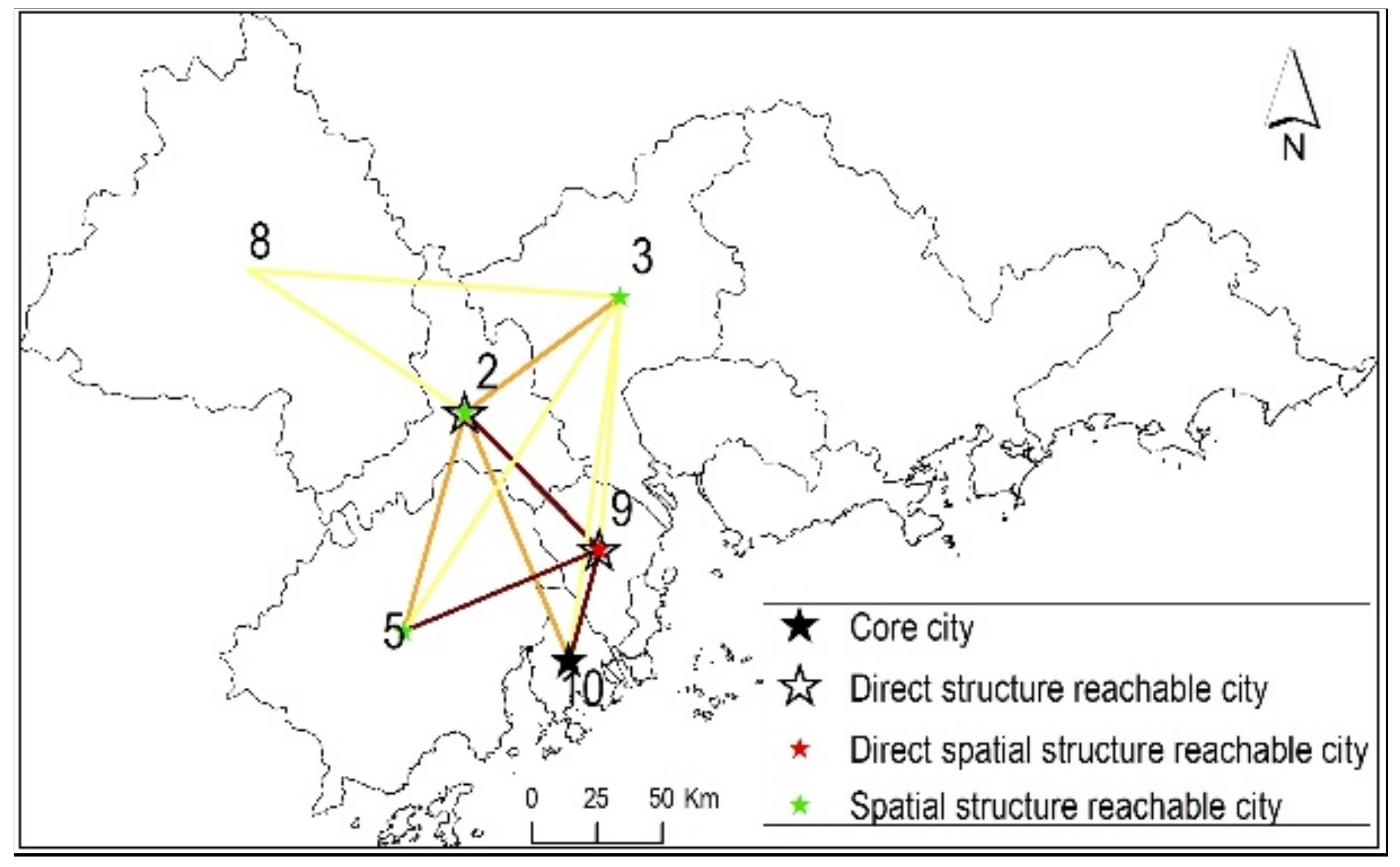
DASSCAN uses core nodes as seeds for expanding communities. A core node and the spatially adjacent nodes in its ε-neighborhood are identified as members of the same community. The idea is formalized in the following definitions. One corresponding example is drawn in Figure 5.
Definition 4.
Direct structure reachability. A node u is directly structurally reachable from node v, if. The direct structure reachable set of a core node v is denoted by.
Definition 5.
Direct spatial structure reachability. A node u is directly spatially and structurally reachable from node v, ifand, denoted by. The direct spatial structure reachable set of a core node v is denoted by.
In fact, is a subset of . The constraint AM(v, u) = 1 in ensures the final spatial community’s connectivity.
Definition 6.
Spatial structure reachability. A node u is spatially and structurally reachable from v, if ∃{v1,…vn} such that v1 = v, vn = u, and ∀i∈{1,2,…,n − 1} such that. This is denoted by.
The spatial structure reachability is transitive, but it is also asymmetric. It is only symmetric for a pair of core nodes. More specifically, the spatial structure reachability is a transitive closure of direct spatial structure reachability. Taking node 10 in Figure 5 as an example, when ε and μ are set to 0.8 and 2, node 10 and three other nodes (2, 5, and 9) are considered core nodes. Node 10’s direct structure reachable nodes are 2 and 9, and only 9 is the direct spatial structure reachable node. In addition, since node 9 is also a core node, node 10 gets two spatial structure reachable nodes, which are 2 and 5. Then, through another core node 2, node 10 gets the third spatial structure reachable node 3.
Two non-core nodes in the same community may not be spatially and structurally reachable because the core condition may not hold for these nodes. However, these two nodes still belong to the same community because they are both structurally reachable from the same core. This idea is formalized in the following definition of spatial structure connectivity.
Definition 7.
Spatial structure connectivity. Two non-core nodes v and u are spatially and structurally connected from a core node w as follows:
Taking Figure 5 as an example, when ε and μ are set to 0.8 and 2, the spatially and structurally connected nodes for node 10 are 2, 3, 5 and 9.
Definition 8.
Spatial structural community. A non-empty subset C⊆V is called a spatial structural community, if all nodes in C are spatially and structurally connected, and C is the maximal with respect to spatial structural reachability as follows:
(1) Connectivity:
(2) Maximally:
Now, we can define a partition of network G with respect to the given parameters ε and μ as all structurally connected communities in G.
Definition 9.
Community partition. A community partition CP of a spatial network G consists of all spatially and structurally connected communities with respect to ε and μ in G as follows:
A node is either a member of a structurally connected community, or it is isolated, i.e., it does not belong to any of the structurally connected communities. If a node is not a member of any structurally connected community, it is either a hub or an outlier, depending on its neighborhood.
Definition 10.
Spatial hub and outlier. Given a community partitionof network G, a node h ∈ V is a spatial hub as follows:
(1) h does not belong to any community:.
(2) h has both a neighborhood connection and spatially adjacent relation with multiple communities:, such that. If a node o∈V does not belong to any community and is not a hub, it is an outlier.
In Figure 1, the two density parameters ε and μ are set to 0.7 and 2. In Figure 3, ε and μ are set to 0.9 and 2, and two communities are found. One community includes nodes 2, 5, 9 and 10, and the other includes nodes 1, 4 and 7. In addition, node 3 is a spatial hub, which bridges the two communities. Nodes 6 and 8 are two outliers.
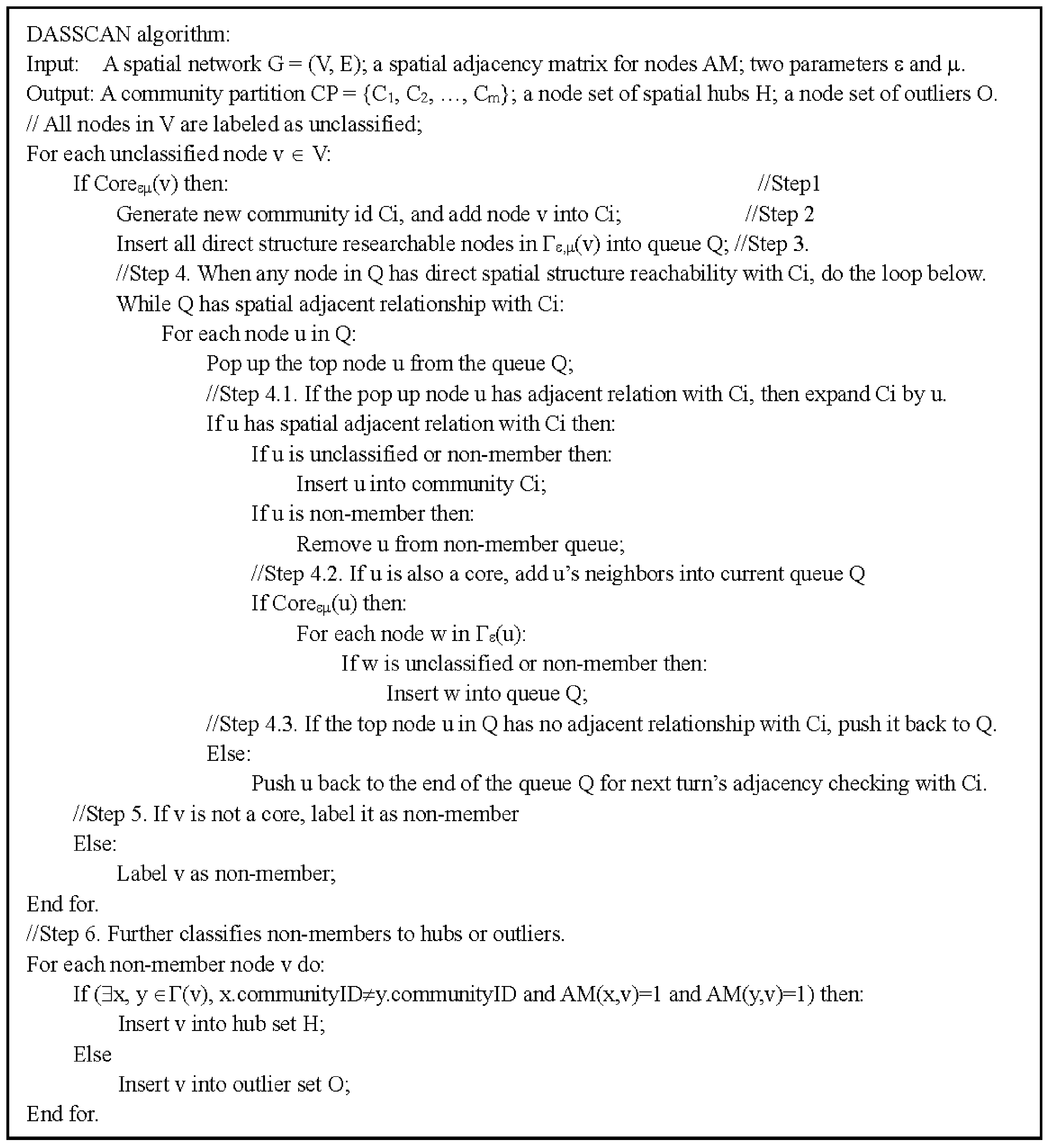
Figure 6 shows the pseudo code of the DASSCAN algorithm. DASSCAN performs an iterative check for each core node of a network and finds all spatially and structurally connected communities, spatial hubs and outliers for the given parameters ε and μ.
At the beginning, all nodes are labeled as unclassified. The DASSCAN classifies each node either as a member of a community or as a nonmember. For each node that is not yet classified, DASSCAN checks whether this node is a core (Step 1 in Figure 4). If the node is a core, a new cluster ID is generated, and a new community is expanded from this node (Step 2). Otherwise, the node is labeled a nonmember (Step 5). To find a new community, DASSCAN starts with an arbitrary core v and searches for all nodes that are structurally reachable from v in Step 3. An iterative spatial structure reachability check is added in Step 4 to ensure the expanding process of the current community is always connected. In Step 4.1, the new cluster ID is assigned to all directly spatially reachable nodes of v. In addition, in Step 4.2, if a node u in the directly spatially reachable node of v is also a core, the u is added to the directly reachable nodes in the queue Q, which are unclassified. Step 4.3 corresponds to Step 4.1. If a node w in a directly structurally reachable set of v has no adjacent relation with the current community Ci, it is placed back into the end of the check queue Q. As the Ci expands in the loop, w may obtain the adjacent relation with Ci in later iterations. The loop in Step 4 will cease when there is no spatially adjacent relation between the nodes in Q and Ci. This iterative adjacency expansion strategy ensures the spatially connected and structurally similar nodes are clustered into one community at most.
The nonmember nodes can be further classified as spatial hubs or outliers in Step 6. If an isolated node has a connection with two or more communities and is adjacent to these communities, the node is classified as a spatial hub. Otherwise, it is an outlier. For more explanation about the roles of hub and outlier nodes in a classical complex network, please refer to [28,29,30]. Since the spatial structure connectivity is a symmetric relation, the results of DASSCAN do not depend on the order of processed nodes, i.e., the obtained community partition of the spatial network is stable.
2.3. Computational Complexity and Efficiency Analysis
DASSCAN has a similar clustering process with DBSCAN, except for the input data structure and the cluster expending strategy. The different cluster strategies do not make any computational complexity. However, the different input data structures have both time and space effects on the two algorithms. The calculation of ε_neighbors is a time-consuming step in DBSCAN. When efficient spatial index structure (e.g., R-tree) is established on the original input data, DBSCAN obtains the average runtime complexity O(n*logn), where n is the number of objects in the dataset. However, in DASSCAN, the relationships between nodes are already exist in the network structure, no extra index is needed. The searching and calculation of ε_neighbors in DASSCAN is direct, and the time complexity is o(1). Thus, the entire time complexity of DASSCAN is o(n). On the other hand, the required space of DASSCAN is much larger than DBSCAN. Network information about the nodes, edges and the adjacent matrix are all needed, so the space complexity of DASSCAN is o(n2).
For DASSCAN, the two density parameters ε and μ have to be specified by the user. Ideally, the value of ε is given by the problem to solve, and μ is then the desired minimum cluster size [33]. However, if the data and scale are not well understood by the user, choosing a meaningful ε can be a difficult task. If the chosen ε is too small, a large part of the data will not be clustered, whereas, for a too high value of ε, clusters will merge and the majority of objects will be in the same cluster. In general, small value of ε is preferable [36]. A more effective method is using k-distance graph to help choose the best value of ε. The k-distance graph plots the distance to the k= μ − 1 nearest neighbor ordered from the largest to the smallest value [33,36], and good values of ε are where this plot shows an “elbow” [33,36,37]. On the other hand, the value of μ can be derived from the number of dimensions (dim) in the dataset, as μ ≥ dim + 1. The low value of μ = 1 does not make sense, as then every point on its own will already be a cluster. Therefore, μ must be at least 2. As a rule of thumb, μ = 2·dim can be used [37]. However, it may be necessary to choose larger values for very large data, for noisy data or for data that contain many duplicates [36], because larger values will yield more significant clusters.
Since the spatial structure connectivity is a symmetric relation, the community results of DASSCAN is usually stable. However, similar to DBSCAN, DASSCAN is not entirely deterministic. The border nodes that are reachable from more than one community can be part of either cluster, depending on the order the data are processed. For most datasets and domains, this situation fortunately does not arise often and has little impact on the clustering result [36]: on both core nodes and noise nodes, DASSCAN is deterministic.
3. Experimental Results
We have implemented DASSCAN in python 2.7 with the NetworkX 2.0 package [38]. NetworkX has well defined data structures for graphs, digraphs, and multigraphs, which can be directly used. All experiments have been run on a computer with an Intel Core i7 processor and 32 GB of Main Memory, running Windows 10.
3.1. A Small Sample Network Experiment
In this section, the inner city, high-speed train network in Guangdong Province is chosen as a sample dataset to test the accuracy and efficiency of the DASSCAN algorithm. Meanwhile, the setting strategy of the DASSCAN parameters are also discussed.
Except for the input network data and adjacency matrix of cities, DASSCAN requires two density parameters to complete the density and adjacency expansion-based spatial network community detection algorithm: the similarity threshold (ε) and minimal number of neighborhood cities (μ). The larger are these two parameters, the greater is the structural similarity in the communities. However, if the original network does not show great similarities between cities, the high parameter values will lead to small community sizes and many outliers will remain.
According to Figure 3, the structural similarities of the sample train network are very high, and their average value is 0.68. Therefore, the similarity threshold ε was chosen from between 0.7 and 0.8, with an interval equal to 0.05. On the other hand, the average degree for all 10 cities is 3.6. Since the community expansion process must consider both connected neighbors and the adjacency constraint, the minimal number of neighborhood cities μ chosen were only 2 and 3 in the experiments. Figure 7 shows the community results using different combinations of the two parameters.
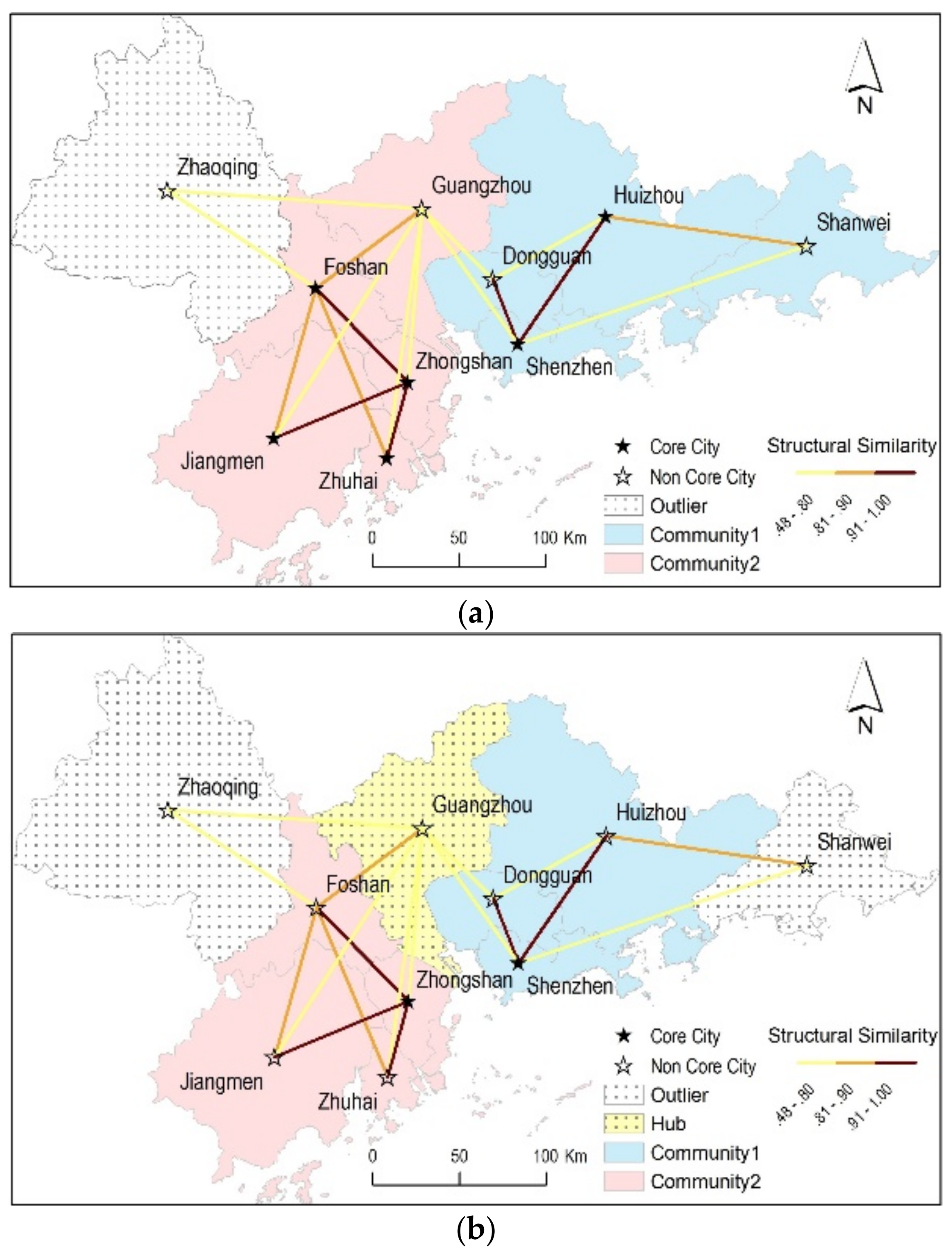
The numbers of communities in Figure 7 show that μ equals 2 is a better choice than 3, because there is only one community found when μ equals 3. In addition, given μ equals 2, the experiments maintain the same community number when ε equals between 0.7 and 0.8. Only when μ equals 2 and ε equals 0.8 is one hub city found by DASSCAN. Figure 8 shows the spatial community results of the sample network data. As shown in Figure 8a, when parameters ε and μ were set to 0.7 and 2, six core cities were found. Then, two communities and one outlier city were found in the west, and no hub was found. On the other hand, as shown in Figure 8b, when ε and μ were set to 0.8 and 2, only two core cities were found. Then, two smaller spatial communities, two outliers and one hub were also found.
Although parameter settings in Figure 8b obtained smaller community sizes, one hidden, valuable hub city (Guangzhou) was discovered. In fact, Guangzhou is the provincial capital of Guangdong Province. Guangzhou acts as a bridge that connects the eastern and western cities. From this standpoint, when parameters ε and μ are set to 0.8 and 2, the sample network obtains the best community results.
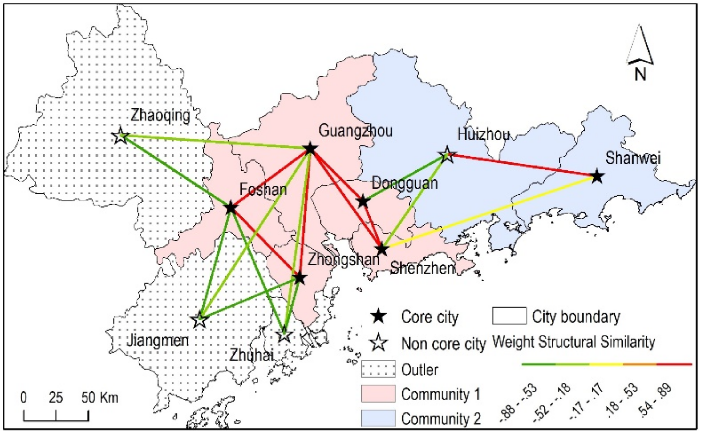
On the other hand, according to Figure 4, the weighted structural similarities of the sample train network have both positive and negative values, and their average value is −0.56. Figure 9 shows the weighted spatial structural community results when parameters ε and μ are set to 0 and 2. Note that, although node 6 has a positive similarity with node 7 and it is a core node, they do not belong to the same community. The reason is they do not have spatial adjacent relation, and they are neither spatial structural reachable nor spatial structural connected.
3.2. A Large Train Network Data Experiment
In this section, the high-speed train network (G-net) in China is used, which contains 159 cities and over 10 thousand edges for the experimental data to test the efficiency of the DASSCAN algorithm on the community detection of a large spatial network. Comparative experiments with the classic SCAN algorithm were also completed.
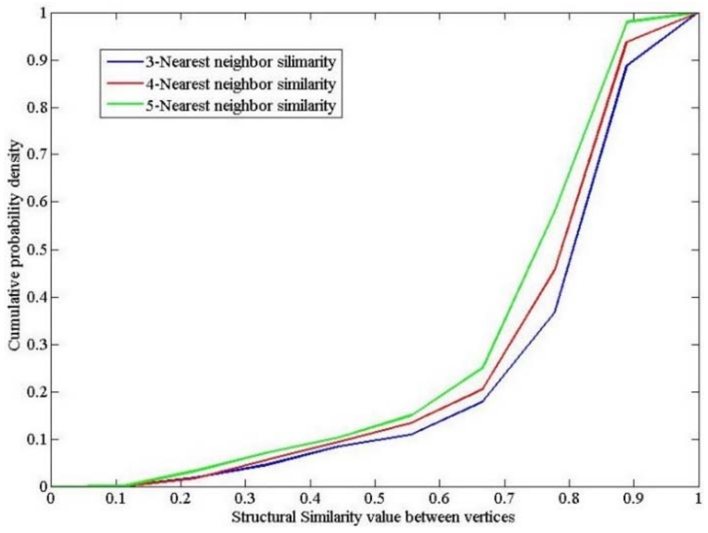
According to the suggested density parameter settings in DBSCAN [33] and SCAN [28], the cumulative probability density (CPD) of the k nearest structural similarity for all nodes is for k equals between 3 and 5, which is shown in Figure 10.
As seen in Figure 10, the structural similarity trend between nodes does not increase much when μ equals between 3 and 5. In addition, the knee of the CPD appears when the structural similarity equals between 0.7 and 0.8. Therefore, the density parameters ε and μ were set to 0.7, 0.75, and 0.8, and 3, 4, and 5, respectively. In addition, two indicators were used to aid in choosing the best parameter combinations.
(1) Community number. Too many communities are confusing and makes it difficult to understand and explain the results. In contrast, when only one community remains, this is also a bad result.
(2) Ratio of the nodes. It is better to have a large ratio of community nodes in the total nodes. For example, over 50 percent is a good ratio. A low ratio means there are too many outliers and hubs in the spatial network, which weakens the differentiation between communities. In addition, the ratio of the largest community’s nodes in all communities’ nodes should not be too large. A ratio that is too large will eliminate the comparability between communities.
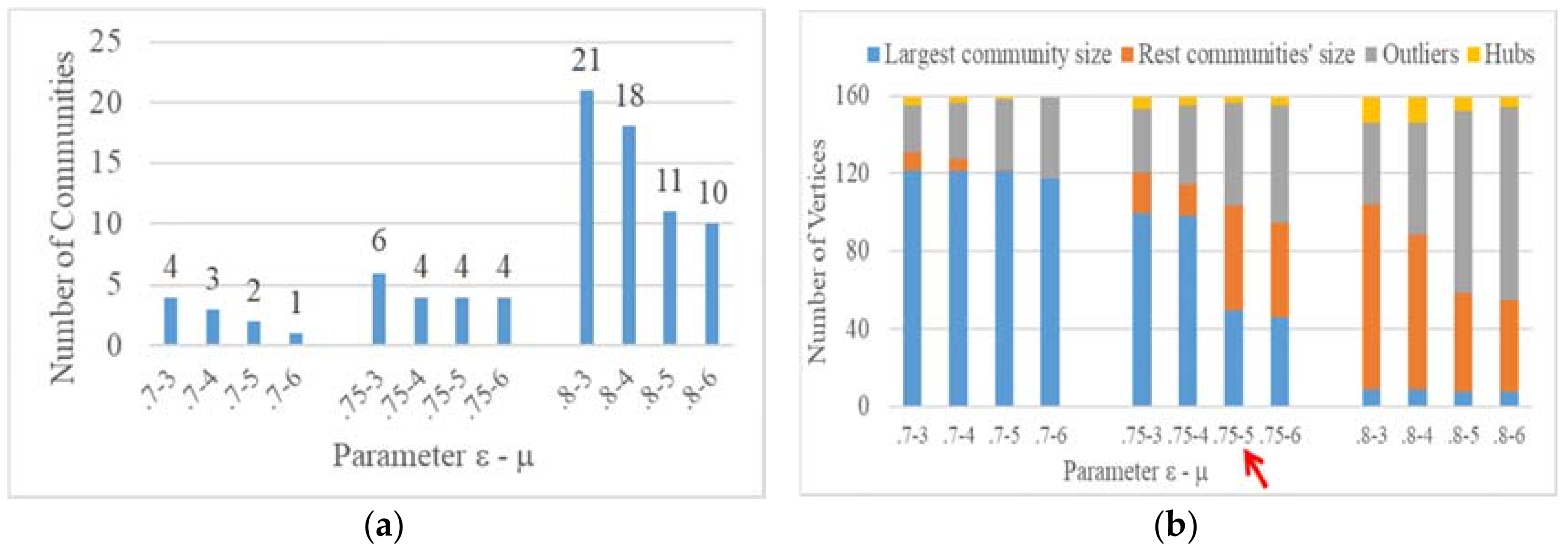
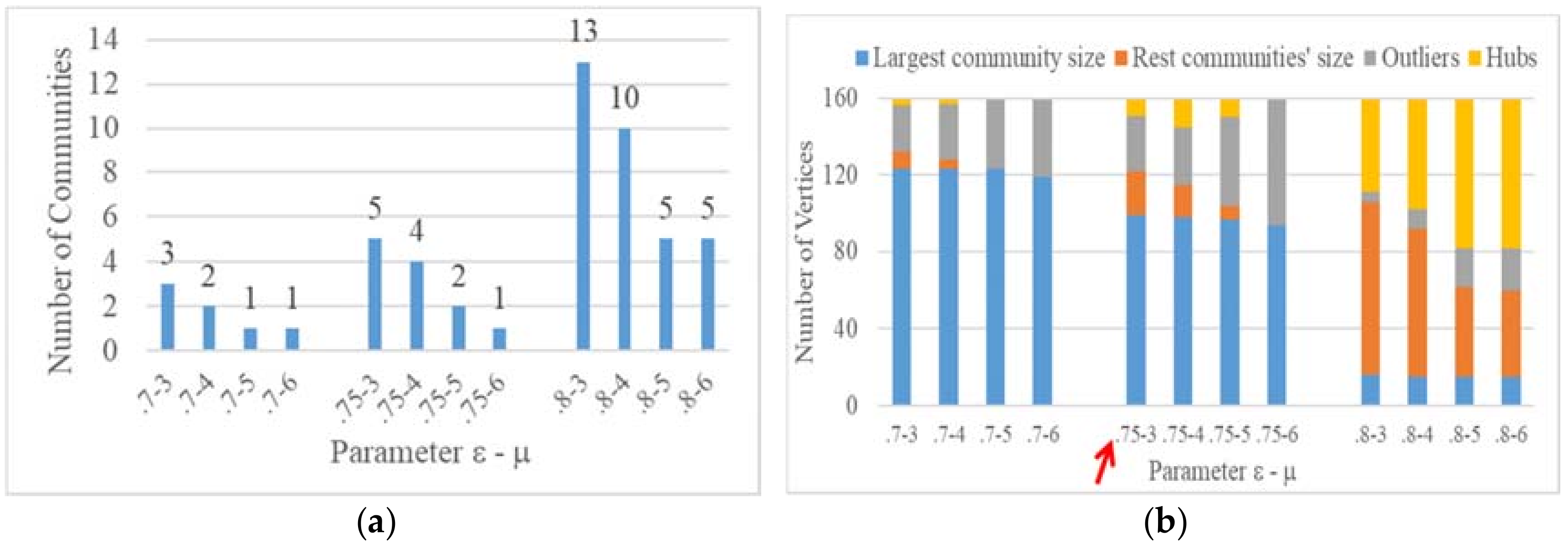
Figure 11 and Figure 12 show the results of the two indicators using different parameter settings for the two algorithms (DASSCAN and SCAN) in the G-net. Based on the parameter choosing criteria stated above, the best parameter combination for DASSCAN is ε = 0.75 and μ = 5, while it is ε = 0.75 and μ = 3 for SCAN.
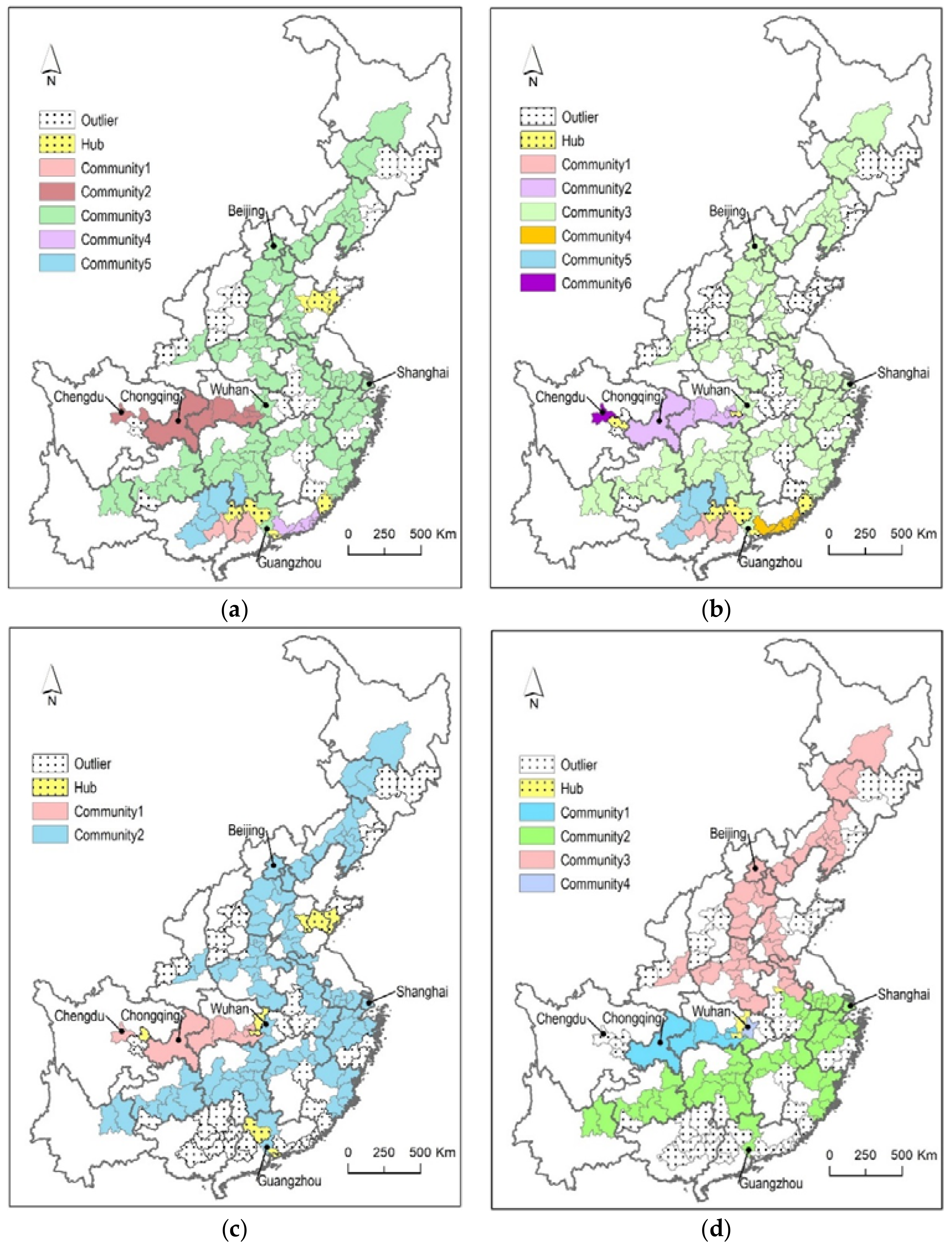
Figure 13 shows the community detection results spatial distributions using two algorithms (DASSCAN and SCAN) and two parameter setting strategies (ε = 0.75, μ = 3, and ε = 0.75, μ = 5) in the G-net.
Some comparative conclusions can be drawn from the community spatial structures and distributions of spatial hubs and outliers:
(1) DASSCAN has better quality community detection results than SCAN. The iterative adjacency expansion strategy of DASSCAN can identify a spatially connected community, which shows a better inner spatial structure. In addition, the structural patterns of all communities are more varied in DASSCAN. When setting suitable density parameters (ε =0.75 and μ = 5), DASSCAN avoids obtaining a large community compared to SCAN. In contrast, DASSCAN identified four interesting communities, which are located in the north, south, west and center of the G-net.
(2) DASSCAN has the same capability as SCAN for finding core nodes in a spatial network, but it has better capability for finding spatial hubs and outliers. The definition of a spatial hub in Section 2.2 has a special constraint, which is a neighborhood connection and spatially adjacent relation between multiple communities. This allows DASSCAN to identify fewer hubs and more outliers than SCAN. As shown in Figure 13a,c, the spatial distribution of hubs found by SCAN does not show interesting patterns. The eastern hubs in Figure 13a and southern hubs in Figure 13c both lack the function of bridging communities in the spatial connection, although they have neighborhood connections with several different communities. Moreover, as the density parameters increase, the number of communities also increases, which leads to over half of the nodes being identified as hubs (as shown in Figure 12b). The community results will be very confusing.
The community results also uncover some accrual meanings that exist in the G-net:
(1) There are three Chinese national central cities in the western and central G-net: Chengdu, Chongqing, and Wuhan. In Figure 13b,d, DASSCAN discovered that Chengdu and Wuhan are two special communities, which both contain only one node. These two cities do not have any high structurally similar cities in their adjacent areas. This indicates that the high-speed train line structure of the two national central cities are not well constructed. The spatial hub cities, which were also discovered by DASSCAN, can be considered the best candidates for improving G-net’s spatial structure.
(2) The distribution of the outlier cities discovered by DASSCAN shows the underdeveloped areas in the G-net, which is especially apparent in the southwestern areas. Figure 13b shows that the inner spatial structural similarities are high, but they do not have intensive connections with nearby communities. Finally, when setting more large density parameters, these parameters are identified as outliers, as shown in Figure 13d. The same suggestion can be made to enhance the connections with the spatial hubs, which are shown in Figure 13b.
4. Conclusions
Community detection is an important and fundamental topic in spatial network studies. Community detection can be used to discover interesting spatial patterns, and aid in understand the spatial structure hidden within networks. However, community detection in spatial networks is quite different from a traditional complex network, since it must consider the effects of spatial constraints (e.g., distance decay and spatial adjacent relation) on spatial community formation. Existing spatial community detection algorithms are usually based on the modularity maximizing strategy. In this study, a novel structural similarity-based spatial network community was defined, which was based on the shared neighbors of nodes. In addition, two other special node roles were defined: spatial hub and outlier. Then, the DASSCAN algorithm was defined to mine these communities, hubs and outliers. DASSCAN does not choose the modularity maximizing strategy. Instead, DASSCAN uses a symmetric measure which is structural similarity to calculate the relationship between nodes, and then, the spatial adjacency expansion strategy and the density-based clustering method are chosen to mine communities. The iterative adjacency expansion strategy ensures the spatially adjacent and structurally similar nodes are clustered into one community at most. The density-based clustering method can always obtain stable community results. Experiments on two kinds of Chinese train line networks clarified the accuracy and efficiency of DASSCAN in finding spatial structural communities, spatial hubs and outliers. Compared to SCAN, which is a classic community detection algorithm used in traditional complex networks, DASSCAN can obtain much better results. The communities found have shown more interesting spatial structural patterns, and the hubs and outliers are more accurate with more valuable meanings. DASSCAN is not only fit for the small train network data, it also can be run on very large size spatial networks efficiently because of its low computational complexity.
On the other hand, DASSCAN also has one shortcoming: the setting of the two density parameters will affect the community results. The k nearest structural similarity calculation on large network is costly. Thus, the future work will start from finding a more flexible parameter setting strategy to improve the DASSCAN.
Acknowledgements
This work was funded through funding from the National Key Research & Development Plan of China (Project Number: 2017YFB0503601) and the National Natural Science Foundation of China (Project Number: 41471327).
Author Contributions
Yaolin Liu conceived the main idea of the study. You Wan designed and performed the experiments, and analyzed the results. You Wan wrote the first version of the paper and both authors revised the manuscript.
Conflicts of Interest
The authors declare that there are no conflicts of interest.
References
- Barthélemy, M. Spatial networks. Phys. Rep. 2011, 499, 1–101. [Google Scholar] [CrossRef]
- Fortunato, S. Community detection in graphs. Phys. Rep. 2010, 486, 75–174. [Google Scholar] [CrossRef]
- Liu, X.; Gong, L.; Gong, Y.X.; Liu, Y. Revealing travel patterns and city structure with taxi trip data. J. Transp. Geogr. 2015, 43, 78–90. [Google Scholar] [CrossRef]
- Austwick, M.Z.; O’Brien, O.; Strano, E.; Viana, M. The structure of spatial networks and communities in bicycle sharing systems. PLoS ONE 2013, 8, e74685. [Google Scholar] [CrossRef]
- Gao, S.; Liu, Y.; Wang, Y.L.; Ma, X.J. Discovering Spatial Interaction Communities from Mobile Phone Data. Trans. GIS 2013, 17(3), 463–481. [Google Scholar] [CrossRef]
- Liu, Y.; Sui, Z.; Kang, C.; Gao, Y. Uncovering patterns of inter-urban trip and spatial interaction from social media check-in data. PLoS ONE 2014, 9, e86026. [Google Scholar] [CrossRef] [PubMed]
- Guimera, R.; Mossa, S.; Turtschi, A.; Amaral, L.N. The worldwide air transportation network: Anomalous centrality, community structure, and cities’ global roles. Proc. Natl. Acad. Sci. USA 2005, 102, 7794–7799. [Google Scholar] [CrossRef] [PubMed]
- Chen, Y.; Xu, J.; Xu, M. Finding community structure in spatially constrained complex networks. Int. J. Geogr. Inf. Sci. 2015, 29, 889–911. [Google Scholar] [CrossRef]
- Ji, Y.; Geroliminis, N. On the spatial partitioning of urban transportation networks. Transp. Res. Part B Methodol. 2012, 46, 1639–1656. [Google Scholar] [CrossRef]
- Anwar, T.; Liu, C.; Vu, H.L.; Leckie, C. Spatial Partitioning of Large Urban Road Networks. In Proceedings of the 17th Inter-National Conference on Extending Database Technology (EDBT), Athens, Greece, 24–28 March 2014; pp. 343–354. [Google Scholar]
- Anwar, T.; Liu, C.; Vu, H.L.; Leckie, C. Partitioning road networks using density peak graphs: Efficiency vs. accuracy. Inf. Syst. 2017, 64, 22–40. [Google Scholar] [CrossRef]
- Barber, M.J.; Fischer, M.M.; Scherngell, T. The community structure of research and development cooperation in Europe: evidence from a social network perspective. Geogr. Anal. 2011, 43, 415–432. [Google Scholar] [CrossRef] [Green Version]
- Guo, D. Regionalization with dynamically constrained agglomerative clustering and partitioning (REDCAP). Int. J. Geogr. Inf. Sci. 2008, 22, 801–823. [Google Scholar] [CrossRef]
- Guo, D. Flow mapping and multivariate visualization of large spatial interaction data. IEEE Trans. Vis. Comput. Graph. 2009, 15. [Google Scholar] [CrossRef]
- Expert, P.; Evans, T.S.; Blondel, V.D.; Lambiotte, R. Uncovering space-independent communities in spatial networks. Proc. Natl. Acad. Sci. USA 2011, 108, 7663–7668. [Google Scholar] [CrossRef] [PubMed]
- Cerina, F.; De Leo, V.; Barthelemy, M.; Chessa, A. Spatial Correlations in Attribute Communities. PLoS ONE 2012, 7. [Google Scholar] [CrossRef] [PubMed] [Green Version]
- Liu, X.; Murata, T.; Wakita, K. Extending Modularity by Incorporating Distance Functions in the Null Model. arXiv 2012, arXiv:1210.4007. [Google Scholar]
- Hannigan, J.; Hernandez, G.; Medina, R.M.; Roos, P.; Shakarian, P. Mining for spatially-near communities in geo-located social networks. In Proceedings of the Association for the Advancement of Artificial Intelligence-Social Networks and Social Contagion: Web Analytics and Computational Social Science, Arlington, VA, USA, 15–17 November 2013. [Google Scholar]
- Shakarian, P.; Roos, P.; Callahan, D.; Kirk, C. Mining for geographically disperse communities in social networks by leveraging distance modularity. In Proceedings of the 19th ACM SIGKDD International Conference on Knowledge Discovery and Data Mining, London, UK, 19–23 August 2018; pp. 1402–1409. [Google Scholar]
- Sarzynska, M.; Leicht, E.A.; Chowell, G.; Porter, M.A. Null models for community detection in spatially embedded, temporal networks. J. Complex Netw. 2015, 4, 363–406. [Google Scholar] [CrossRef]
- Cazabet, R.; Borgnat, P.; Jensen, P. Enhancing space-aware community detection using degree constrained spatial null model. In Proceedings of the Workshop on Complex Networks CompleNet, Dubrovnik, Croatia, 21–24 March 2017; pp. 47–55. [Google Scholar]
- Newman, M.E. Fast algorithm for detecting community structure in networks. Phys. Rev. E 2004, 69, 066133. [Google Scholar] [CrossRef] [PubMed]
- Newman, M.E.; Girvan, M. Finding and evaluating community structure in networks. Phys. Rev. E 2004, 69, 026113. [Google Scholar] [CrossRef] [PubMed]
- Bakillah, M.; Li, R.Y.; Liang, S.H.L. Geo-located community detection in Twitter with enhanced fast-greedy optimization of modularity: the case study of typhoon Haiyan. Int. J. Geogr. Inf. Sci. 2015, 29, 258–279. [Google Scholar] [CrossRef]
- Good, B.H.; de Montjoye, Y.-A.; Clauset, A. Performance of modularity maximization in practical contexts. Phys. Rev. E 2010, 81, 046106. [Google Scholar] [CrossRef] [PubMed]
- Blondel, V.D.; Guillaume, J.-L.; Lambiotte, R.; Lefebvre, E. Fast unfolding of communities in large networks. J. Stat. Mech. Theory Exp. 2008, 2008, P10008. [Google Scholar] [CrossRef]
- Sobolevsky, S.; Campari, R.; Belyi, A.; Ratti, C. General optimization technique for high-quality community detection in complex networks. Phys. Rev. E 2014, 90, 012811. [Google Scholar] [CrossRef] [PubMed]
- Xu, X.; Yuruk, N.; Feng, Z.; Schweiger, T.A. Scan: A structural clustering algorithm for networks. In Proceedings of the 13th ACM SIGKDD International Conference on Knowledge Discovery and Data Mining, San Jose, CA, USA, 12–15 August 2007; pp. 824–833. [Google Scholar]
- Scripps, J.; Tan, P.-N.; Esfahanian, A.-H. Node roles and community structure in networks. In Proceedings of the 9th WebKDD and 1st SNA-KDD Workshop on Web Mining and Social Network Analysis, San Jose, CA, USA, 12–15 August 2007; pp. 26–35. [Google Scholar]
- Papadopoulos, S.; Kompatsiaris, Y.; Vakali, A.; Spyridonos, P. Community detection in social media. Data Min. Knowl. Discov. 2012, 24, 515–554. [Google Scholar] [CrossRef]
- Tiedaobu. Available online: http://www.12306.cn/mormhweb/ (accessed on 20 March 2018).
- Seaton, K.A.; Hackett, L.M. Stations, trains and small-world networks. Phys. A Stat. Mech. Its Appl. 2004, 339, 635–644. [Google Scholar] [CrossRef]
- Ester, M.; Kriegel, H.-P.; Sander, J.; Xu, X. A density-based algorithm for discovering clusters in large spatial databases with noise. In Proceedings of the Second International Conference on Knowledge Discovery and Data Mining (KDD), Portland, OR, USA, 2–4 August 1996; pp. 226–231. [Google Scholar]
- Sarwar, B.; Karypis, G.; Konstan, J.; Riedl, J. Item-based collaborative filtering recommendation algorithms. In Proceedings of the 10th International Conference on World Wide Web, Hong Kong, China, 1–5 May 2001; pp. 285–295. [Google Scholar]
- Aggarwal, C.C. Recommender Systems; Springer: Berlin, Germany, 2016. [Google Scholar]
- Schubert, E.; Sander, J.; Ester, M.; Kriegel, H.P.; Xu, X. DBSCAN Revisited, Revisited: Why and How You Should (Still) Use DBSCAN. ACM Trans. Database Syst. 2017, 42. [Google Scholar] [CrossRef]
- Sander, J.; Ester, M.; Kriegel, H.-P.; Xu, X. Density-based clustering in spatial databases: The algorithm gdbscan and its applications. Data Min. Knowl. Discov. 1998, 2, 169–194. [Google Scholar] [CrossRef]
- NetworkX. Available online: https://networkx.github.io/ (accessed on 20 March 2018).
Figure 1.
A sample spatial network and its structural communities.

Figure 2.
The two topological models for railway nets: (a) space L model; and (b) space P model.

Figure 3.
The structural similarity and core nodes in the sample train network.

Figure 4.
The weighted structural similarity and core nodes in the sample train network.

Figure 5.
The Spatial structure reachable cities of core city 10.

Figure 6.
The Pseudo code for the DASSCAN algorithm.

Figure 7.
The spatial structural communities in the sample network using different parameters.

Figure 8.
Different parameter settings for DASSCAN in the sample inner city train network: (a) ε = 0.7, μ = 2; and (b) ε =0.8, μ =2.
Figure 8.
Different parameter settings for DASSCAN in the sample inner city train network: (a) ε = 0.7, μ = 2; and (b) ε =0.8, μ =2.

Figure 9.
The community results of DASSCAN in the sample inner city train network by using weighted spatial structural similarity.
Figure 9.
The community results of DASSCAN in the sample inner city train network by using weighted spatial structural similarity.

Figure 10.
The cumulative probability density of the structural similarity between G-net nodes.

Figure 11.
Different parameter settings for DASSCAN on the high-speed train network: (a) number of communities; and (b) ratio of nodes.
Figure 11.
Different parameter settings for DASSCAN on the high-speed train network: (a) number of communities; and (b) ratio of nodes.

Figure 12.
Different parameter settings for SCAN on the high-speed train network: (a) number of communities; and (b) ratio of nodes.
Figure 12.
Different parameter settings for SCAN on the high-speed train network: (a) number of communities; and (b) ratio of nodes.

Figure 13.
Community results for SCAN and DASSCAN in the high-speed train network: (a) SCAN (ε = 0.75, μ = 3); (b) DASSCAN (ε = 0.75, μ = 3); (c) SCAN (ε = 0.75, μ = 5); and (d) DASSCAN (ε = 0.75, μ = 5).
Figure 13.
Community results for SCAN and DASSCAN in the high-speed train network: (a) SCAN (ε = 0.75, μ = 3); (b) DASSCAN (ε = 0.75, μ = 3); (c) SCAN (ε = 0.75, μ = 5); and (d) DASSCAN (ε = 0.75, μ = 5).


Table 1.
Sample train lines data for two kinds of train types.
| Train Number | Train Type | Nodes |
|---|---|---|
| C1001 | Intercity high-speed train | Changchun, Jilin, Yanbian. |
| G1 | High-speed train | Beijing, Nanjing, Shanghai. |
Table 2.
The number of nodes and edges for the train line networks.
| Network | Cities/Nodes | Connections | Average Degree of Node | Average Adjacent Cities for Each Node |
|---|---|---|---|---|
| C-net | 35 | 98 | 2.8 | 2.2 |
| G-net | 159 | 10,040 | 63.1 | 3.8 |
© 2018 by the authors. Licensee MDPI, Basel, Switzerland. This article is an open access article distributed under the terms and conditions of the Creative Commons Attribution (CC BY) license (http://creativecommons.org/licenses/by/4.0/).
Share and Cite
MDPI and ACS Style
Wan, Y.; Liu, Y. DASSCAN: A Density and Adjacency Expansion-Based Spatial Structural Community Detection Algorithm for Networks. ISPRS Int. J. Geo-Inf. 2018, 7, 159. https://0-doi-org.brum.beds.ac.uk/10.3390/ijgi7040159
AMA Style
Wan Y, Liu Y. DASSCAN: A Density and Adjacency Expansion-Based Spatial Structural Community Detection Algorithm for Networks. ISPRS International Journal of Geo-Information. 2018; 7(4):159. https://0-doi-org.brum.beds.ac.uk/10.3390/ijgi7040159
Chicago/Turabian StyleWan, You, and Yaolin Liu. 2018. "DASSCAN: A Density and Adjacency Expansion-Based Spatial Structural Community Detection Algorithm for Networks" ISPRS International Journal of Geo-Information 7, no. 4: 159. https://0-doi-org.brum.beds.ac.uk/10.3390/ijgi7040159
Note that from the first issue of 2016, this journal uses article numbers instead of page numbers. See further details here.