1. Introduction
Space-Filling Curves (SFC) map a compact interval to a multidimensional space by passing through every point of the space. They exhibit good locality preservation properties that make them useful for partitioning or reordering data and computations [
1,
2]. Therefore, SFCs have been widely used in a number of applications, including parallel computing [
3,
4], file storage [
5], database indexing [
6,
7,
8], and image retrieval [
9,
10]. SFCs have been also proven a useful solution for massive points management [
11]. It first maps spatial data objects into one-dimensional (1D) values and then indexes those values using a one-dimensional indexing technique, typically the B-tree. SFC-based indexing requires only mapping functions and incurs no additional efforts in current databases compared with conventional spatial index structures.
Although many classical SFC generation methods have been put forward—recursive, byte-oriented, and table-driven—these methods mainly focused on the efficient generation of n-dimensional (nD) SFC values. Very little existing work focus on efficient query support with SFC values [
12,
13], so there are no complete nD SFC libraries available both for mapping and query. Furthermore, when faced with millions of input points, serial generation of space-filling curves will hinder scalability. In order to improve scalability, a parallel SFC library is needed for practical use.
To address the above-mentioned problems of completeness, universality, and scalability, a generic nD SFC library is proposed and validated in massive multiscale nD point management (open source available from
http://sfclib.github.io/). Designed with object-oriented programming (OOP), it provides abstract objects for SFC encoding/decoding, pipeline bulk loading, and nD box queries. The library currently supports two well-known types of SFC—Morton and Hilbert curves—but could be easily extended to other types. During implementation, the SFC library exploits the parallelism of multicore CPU processors to accelerate all the SFC functions.
The application of this nD SFC library to massive point cloud management was carried out on a bulk loading and geometry query. During bulk loading, a random level of detail (LOD) value l is calculated for each point, following a data pyramid distribution in a streaming mode. This LOD value l is treated as the 4th dimension added to the xyz coordinates. A unique SFC key is also generated with the proposed SFC library for point clustering. Then, only the generated keys are stored as flat records in an Oracle Index Organized (IOT) table without repeating the original values for x, y, z, and l as they can be completely obtained from the key value (by the decode function). This key-only storage schema is much more compact and achieves better data compression. The nD range query is also conducted with the help of these unique SFC keys.
Loading and query experiments show that the proposed nD SFC library is very efficient, exhibiting robust scalability over massive point datasets. For example, when loading 23 billion LiDAR (Light Detection and Ranging) points into Oracle, the parallel mode takes only 10 h, and the loading speed is an estimated four times faster than sequential loading. Further, 4D queries with Hilbert keys take about 1~5 s and scale well the input data size.
The rest of the paper is organized as follows. A general description of the Space-Filling Curve and a review of current nD indexing/clustering methods are presented in
Section 2.
Section 3 explains the fundamentals of our proposed generic nD SFC library and the application of our SFC library to massive multiscale point management.
Section 4 provides the results of load and query performance evaluation and
Section 5 discusses the obtained results.
Section 6 presents conclusions and future research directions.
2. Related Work
2.1. Space-Filling Curves and Current Implementations
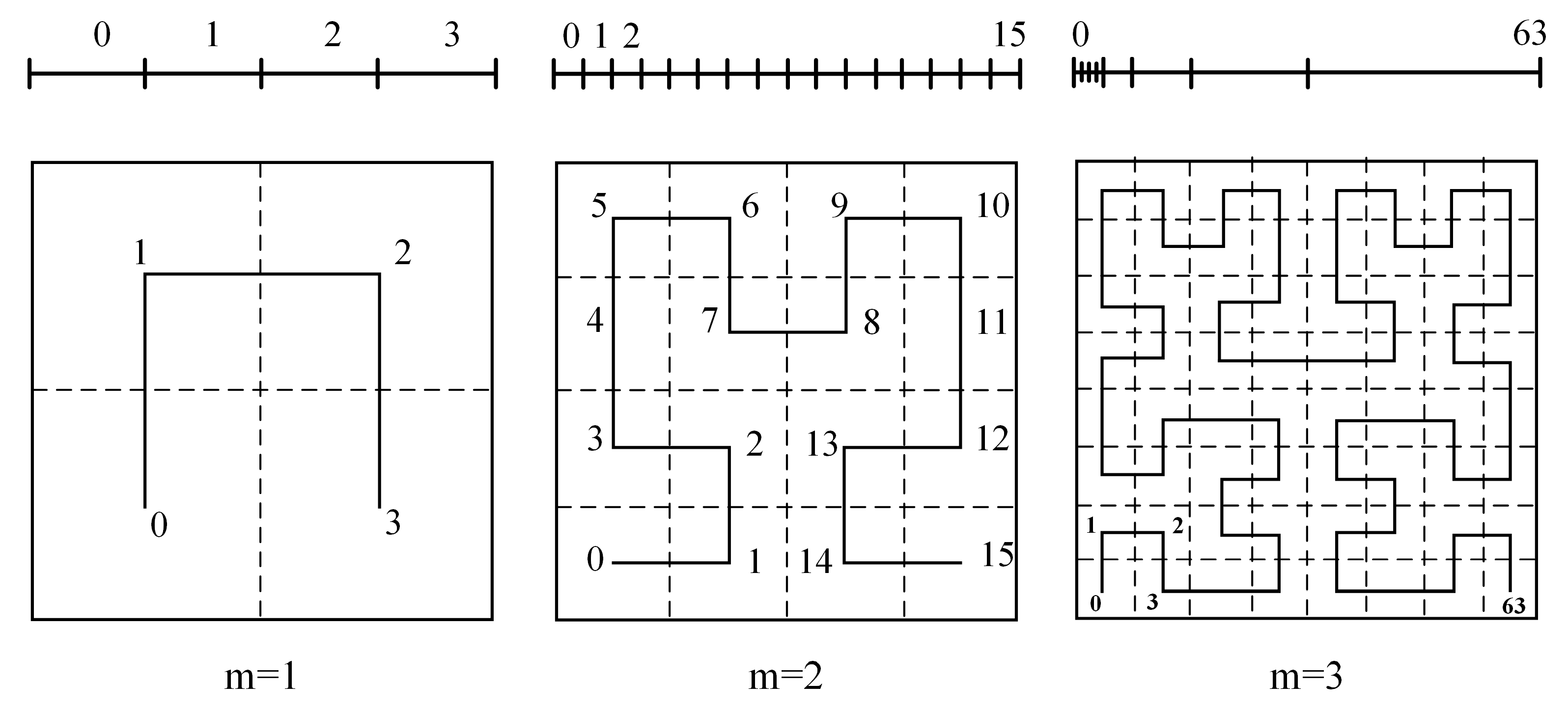
In mathematics, a space-filling curve is a continuous bijection from the hypercube in nD space to a 1D line segment, i.e.,
[
14]. The nD hypercube is of the order
m if it has a uniform side length 2
m. Analogously, the curve
C also has an order
m and its length equals to the total number of 2
n*m cells, shown in
Figure 1.
Point-to-point mapping (encoding/decoding) and box-to-segment mapping (querying) functions are both needed for normal SFC applications. For point-to-point mapping functions, three types of classical SFC generation methods have been put forward: recursive, byte-oriented, and table-driven. Because of self-similarity, recursive generation of space-filling curves in lower dimensional spaces has been extensively studied [
14,
15]. Butz’s byte-oriented algorithm uses several bit operations such as Shifting and Exclusive OR, and can be theoretically applied to any-dimension numbers [
7,
16]. Table-driven algorithms define a look-up table first to quickly generate multidimensional SFCs on the fly [
17]. However, the structure of the look-up table will be quite complicated when extended to higher dimensions, e.g., 4D+.
For box-to-segment mapping functions, few works have been carried out; those that have can be categorized as iterative and recursive. The iterative algorithms find target intervals of curve values in an iterative way by repeatedly calling two functions: one function to compute the next SFC value inside the window and another function to compute the next SFC value outside the window query [
12]. Wu presented an efficient algorithm for 2D Hilbert curves by recursively decomposing the query window [
13]. The latter type is much more efficient than the former one, but it is sequential and limited to the 2D case; we should extent it to nD support and parallel mode.
2.2. Massive LiDAR Point Cloud Management
With the development of spatial acquisition technologies such as airborne or terrestrial laser scanning, point clouds with millions, billions, or even trillions of points are now generated [
18]. Each point in these point datasets contains not only 3D coordinates but also other attributes, such as intensity, number of returns, scan direction, scan angle, and RGB values. These massive points can therefore be understood and treated as typical multidimensional data, as each point record is an
n-tuple. Storage, indexing, and query on these massive multidimensional points poses a big challenge for researchers [
19].
Traditional file-based management solutions store point data in specific formats (e.g., ASPRS LAS), but data isolation, data redundancy, and application dependency in such data formats are major drawbacks. The Database Management System (DBMS)-based solutions can be categorized into two types [
11]: block and flat-table models. In the block model, the point datasets are partitioned into regular tiles, and each tile is stored as a binary large object (BLOB). Some common relational databases, e.g., Oracle and PostgreSQL, even provide intrinsic abstract objects and SQL extensions for this type of storage model. The open-source library PDAL (Point Data Abstraction Library) can facilitate the manipulation of blocked points in these databases. In the flat-table model, points are directly stored in a database table, one row per point, resulting in tables with many rows [
20]. Three columns in a table store X/Y/Z spatial coordinates, while other columns accommodate additional attributes. This flat-table model is easy to implement and very flexible for query and manipulation. However, there are no efficient indexing/clustering methods available for high-dimensional datasets in the currently used relational databases.
2.3. nD Spatial Indexing Methods
Existing nD spatial indices can be classified into two categories: explicit dynamic trees and implicit fixed trees.
An explicit dynamic tree for nD cases maintains a dynamic balanced tree and adaptively adjusts the index structures according to input features to produce a better query performance [
21,
22]. However, this adjustment will degrade index generation performance, especially when faced with concurrent insertions. This category includes the R-tree and its variants, illustrated in
Figure 2.
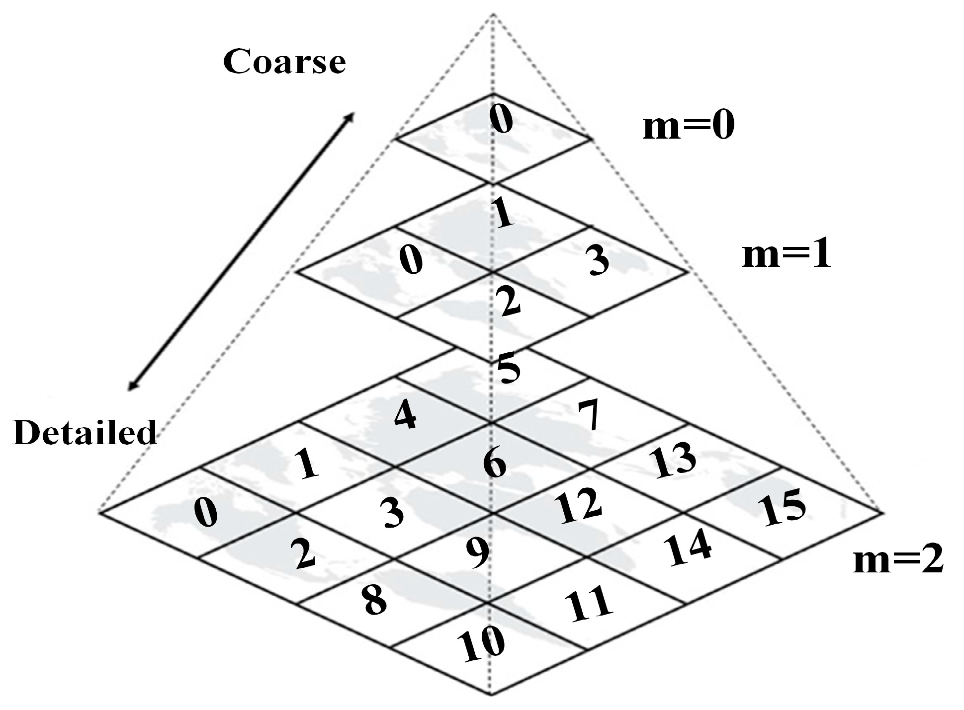
An implicit fixed tree for nD cases relies on predefined space partitioning, such as grid-based methods [
23] and Space-Filling Curves, as illustrated in
Figure 3. For example, Geohash [
24], as a Z-order curve, recursively defines an implicit quadtree over the worldwide longitude–latitude rectangle and divides this geographic rectangle into a hierarchical structure. Then, GeoHash uses a 1D Base32 string to represent a 2D rectangle for a given quadtree node. GeoHash is widely implemented in many geographic information systems (e.g., PostGIS), and is also used as a spatial indexing method in many NoSQL databases (e.g., MongoDB, HBase) [
25].
Indices based on implicit fixed trees have benefits over explicit dynamic tree methods in two respects. Firstly, the 1D indexing methods, e.g., B-tree, are very mature and are supported in all commercial DBMSs. Thus, this type of mapping-based index can be easily integrated into any existing DBMS (SQL or NoSQL, even without spatial support). No additional work is required to modify the index structure, concurrency controls, or query execution modules in the underlying DBMS. Secondly, an implicit fixed tree does not need to build a whole division tree in practical use. When calculating indexing keys, it only needs the coordinates of each point without involving other neighboring points. It is much more scalable for managing large-volume point datasets.
3. Materials and Methods
3.1. The Generic nD SFC Library
3.1.1. The Design of the nD SFC Library
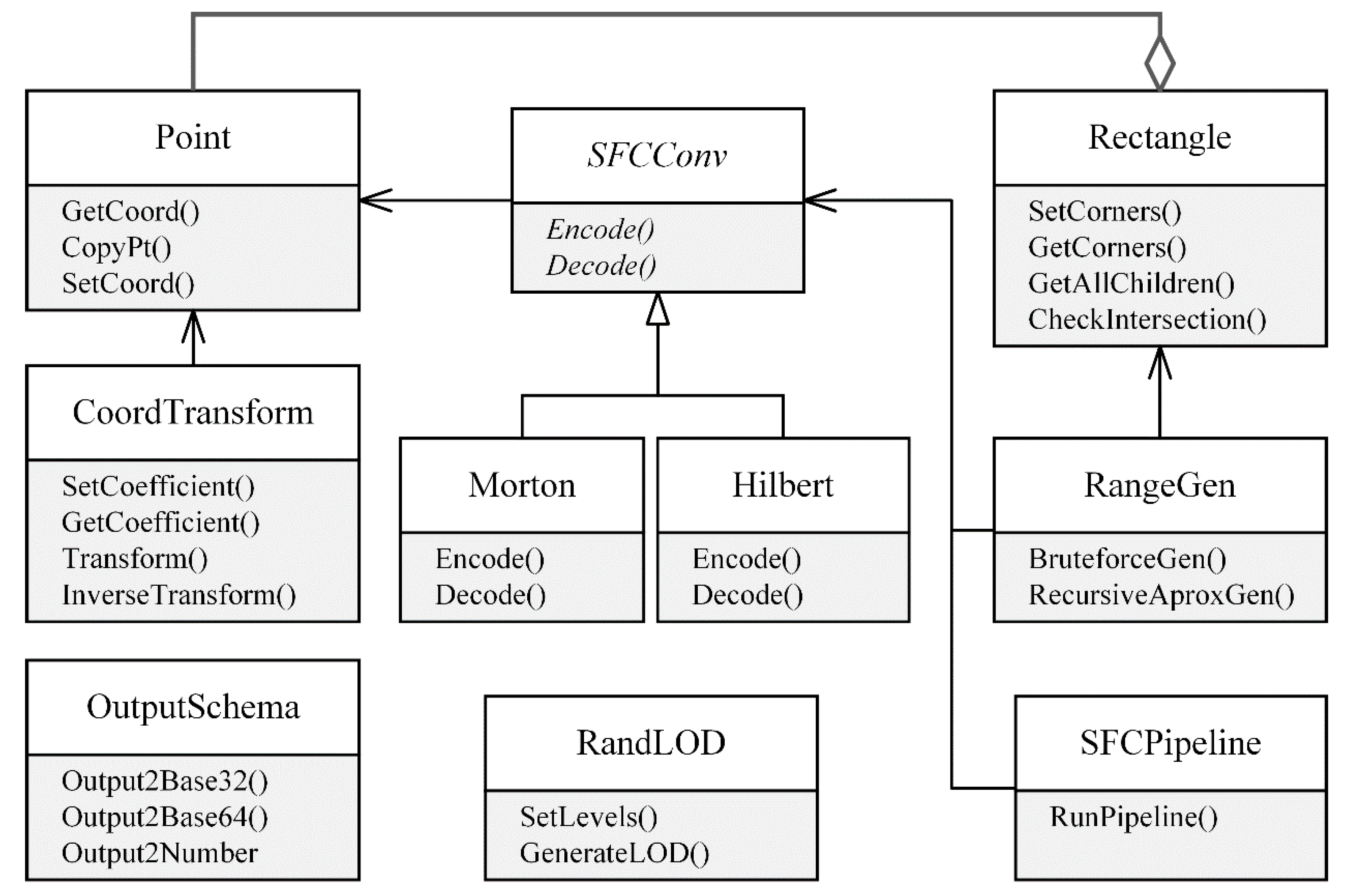
The open-source generic nD SFC library was designed in consideration of object-oriented programming and implemented with C++ template features. This allows library codes to be structured in an efficient way to enhance readability, maintainability, and extensibility. The components of this SFC library are illustrated in
Figure 4. It contains general data structures (e.g., Point and Rectangle), core SFC-related classes (e.g., CoordTransform, SFCConv, OutputSchema, RangeGen, and SFCPipeline), and other auxiliary objects (e.g., RandLOD).
The Point class is used to represent the input points for SFC encoding/decoding, while the Rectangle class supports nD range queries with SFC keys. Both classes are generic and easily extended to any dimensions.
The CoordTransform class converts the coordinates between geographic space and SFC space, i.e., from float type to integer type. Two transformation modes are supported here: translation and scaling. During coordinate transformation, users first define the translation distances and the scaling coefficients, which can be different for each dimension.
The abstract SFCConv class can be inherited to implement different SFC curves and provides the interface for SFC encoding/decoding. This class converts the input SFC space coordinates into a long bit sequence, and then the bit sequence will be encoded into the target code type, e.g., 256-bit number or hash string by the OutputSchema class. The OutputSchema class also supports different string schemas, e.g., Base32 or Base64. The RangeGen class provides the required range query interfaces through which the users input an nD box and a set of 1D SFC ranges are outputted.
Currently, the SFC Library implements two types of SFC curves: Morton/Z-order and Hilbert. The Morton curve only interleaves the input SFC coordinates, so its encoding and decoding is trivial. Butz and Lawder’s byte-oriented methods are used for efficient Hilbert encoding/decoding [
7,
14,
16]. The details of Hilbert encoding/decoding are presented in
Appendix A.
3.1.2. The nD Box Query with SFC Keys
The objective of an nD box query can be stated as follows: Given an
Rn input box
B defined by min and max coordinates in every dimension, the query operation
Q(
B) returns those points
Sk which are fully contained by the nD box
B. Because all points are indexed with 1D SFC keys, the box query is equivalent to translating nD input box
B into a collection of 1D SFC key ranges
K and filtering target points using these derived key ranges.
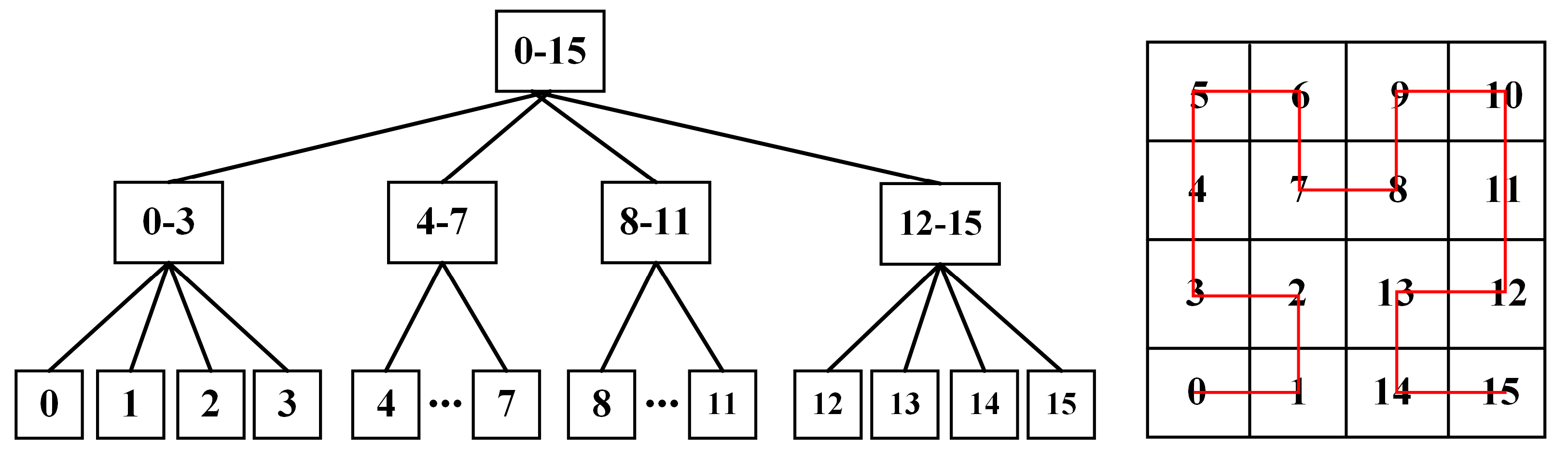
The space-filling curve can be treated as a space partitioning method. The target nD space is divided into a collection of grid cells recursively until the level of space partitioning reaches
m. Each cell is labeled by a unique number which defines the position of this cell in the space-filling curve. The space partitioning process by a space-filling curve can be represented by a complete 2
n-ary tree (i.e., for 2D is a quadtree; for 3D is an octree). Every tree node in this implicit 2
n-ary tree covers an nD box and can be translated to an SFC range. This process is illustrated in
Figure 5.
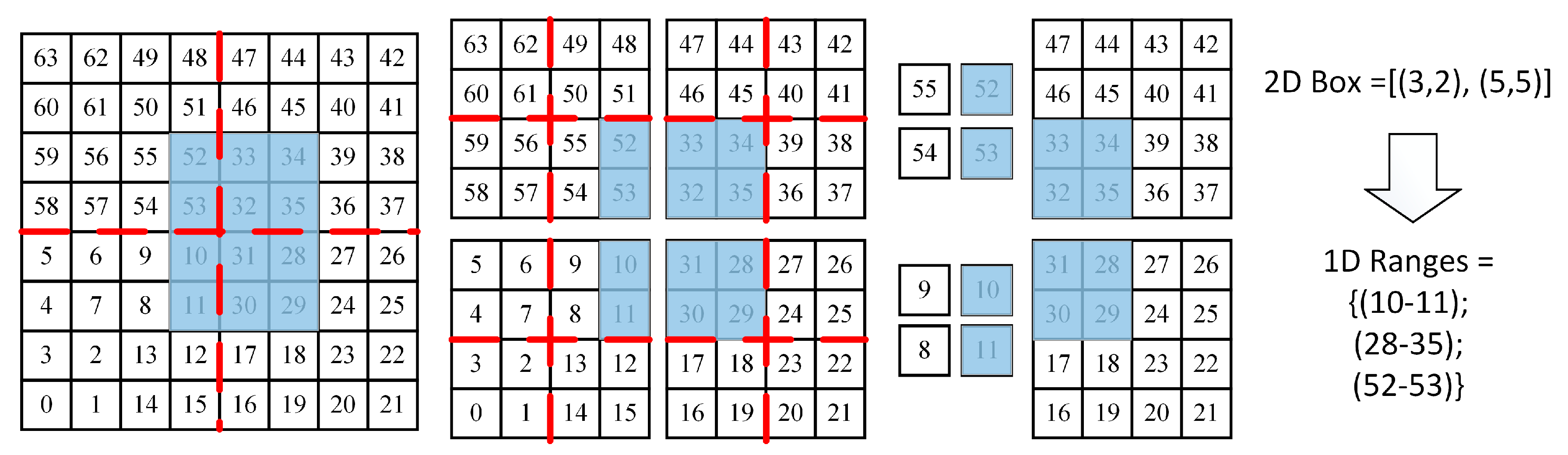
A recursive range generation method is proposed following this feature. The core idea of this recursive method is to recursively approximate the input nD box with different levels of tree nodes. So, the original objective is further transformed and restated as finding a collection of tree nodes whose combination is equal to the input nD box. The recursive range generation algorithm is explained as follows and also illustrated in
Figure 6.
Start from the root tree node;
Get all 2n child nodes;
Fetch one child node and check the spatial relationship between the input box and this child node:
- ➢
If it equals to this child, stop here and output this child node;
- ➢
If it is contained by this child, go down from this child node directly and repeat 2;
- ➢
If it is intersected by this child, bisect the input box along the middle line in each dimension and obtain new query boxes;
- ➢
If no overlap, repeat 3 and check other child nodes.
Repeat 2 and 3 with intersected children nodes and new query boxes until the leaf level;
Translate the obtained nodes into SFC ranges, merge continuous intervals, and return the derived ranges.
The tree nodes thus obtained will be later translated to 1D ranges to fetch the required points. For higher-resolution SFCs, the number of 1D ranges usually exceeds thousands or even millions. Due to the sparsity of points in SFC cells, most 1D ranges will not filter any point, while too many ranges take a long time to load and filter. Therefore, additional tree traversal depth control and adjacent range merge are conducted before returning ranges. Because tree traversal is done in a breadth-first manner, when the traversal goes down to a new level, the number of currently obtained nodes is checked as to whether it is bigger than K*N (N is the number of returned ranges; K is the extra coefficient). If it exceeds K*N, the traversal is terminated. Thus, Step 5 of the recursive range generation will be extended as:
Get all raw ranges from each tree node (number ≥ K*N);
Sort all the gap distances from raw ranges;
Get the nth gap distance (the default value is 1);
Merge all the gaps which are less than/equal to the nth gap distance.
3.1.3. The Parallelization of the Generic nD SFC Library
Applications of this generic nD SFC library usually face massive datasets; therefore, the available parallelism of multicore processors is exploited to accelerate practical use. Profiling demonstrates that the two most compute-intensive steps are SFC key encoding when bulk loading, and SFC range generation for nD box queries.
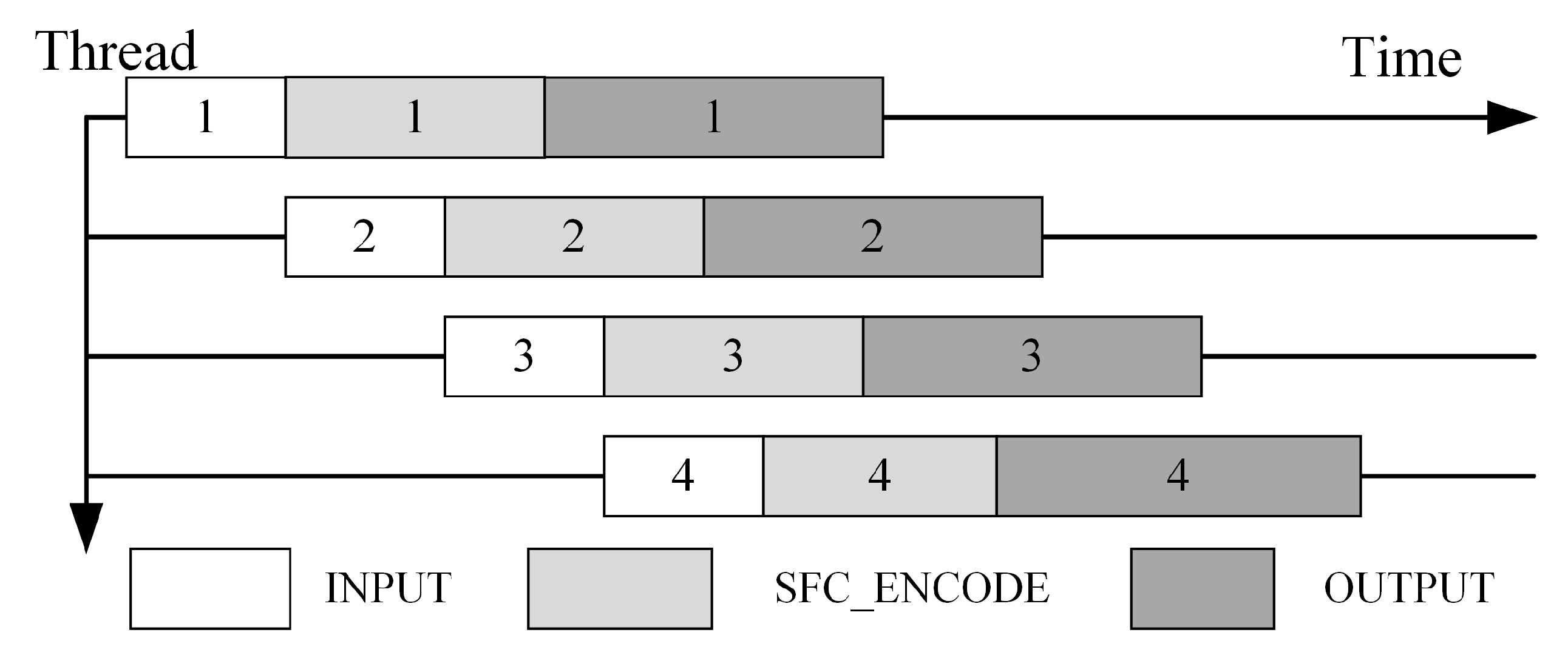
For bulk SFC encoding, a raw point dataset is usually two or three orders of magnitude larger than the memory of standard computing hardware. The points cannot be loaded into main memory to generate the SFC keys one by one. Pipelining is adopted to fetch data sequentially into the memory to support thread-level parallelism.
Figure 7 illustrates our pipeline design for bulk SFC encoding, in which parallelism is designed at the pipeline level. Each pipeline includes three continuous stages: INPUT, SFC_ENCODE, and OUTPUT. The chunk size of the INPUT stage determines how many points are read and encoded in each pipeline. Another feature of this pipelining is overlapped I/O, i.e., when one thread is blocked by the I/O operation, others threads can continue the encoding work. All bulk SFC encoding pipelines are implemented with the Intel Threading Building Blocks (Intel TBB) [
26,
27].
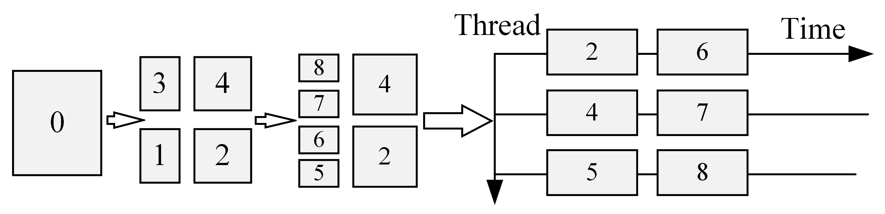
During the translation from the nD box into discrete 1D ranges for nD range query, a collection of discrete tree nodes is obtained; each tree node is further translated into an SFC line segment. These discrete tree nodes are then dispatched to concurrent threads and each thread will take the burden of one part of tree nodes, as illustrated in
Figure 8.
3.2. The Application of the Proposed SFC Library in Massive Multiscale Points Management
3.2.1. Random LOD Generation
During visualization, due to massive data size, multiple levels of detail are usually created to allow users to select only a certain percentage of points in a query region. Traditionally, a collection of discrete LODs is derived in an iterative way from the bottom level to the top level; this is called
Uniform Sampling [
28].
In Uniform Sampling, the original datasets are treated as the bottom level, and the points in one level i + 1 are sampled by a uniform random selection to the upper level i. The factor between two adjacent levels can be 2n, i.e., one in every 2n +1 points of level i + 1 will be randomly selected into the level i. The drawback of this method is that it’s order-dependent and therefore does not perform well in a parallel mode.
To avoid point counting, an alternative streaming method is proposed based on probabilities of an ideal pyramid distribution among all levels. Assume that there are a total of 32 levels, and that the lowest level is
l = 31 (most detailed, highest number of points) and the highest level is
l = 0 (least detailed, fewest points); then the number of points in an ideal pyramid distribution for each level will be
The total
l probability intervals are derived as
A uniform random variable
is then defined. The
X will generate a random value
x for each point in the stream, and the generated
x will then be checked for the probability interval it falls in. This will be used as the LOD level number for this point. The assignment process is illustrated in
Figure 9.
A total of 32 levels should be enough for any dataset. For a given dataset, 32 levels may be too much and, using the random distribution as described, most of the top levels will be empty. However, it may happen in rare cases that a point is assigned to such a top level, and in such a case the point is reassigned to a lower level.
3.2.2. Loading and Indexing with nD SFC Keys
Since all the input point clouds are available as LAS/LAZ files, the loading uses LAStools to convert LAS/LAZ files to ASCII text records. The text records are then inserted into a temporary Oracle heap table with the sqlldr tool and later clustered into an Oracle IOT table using the SFC keys. The IOT table is contrary to a normal heap table, which requires an additional index to be created. This decreases the storage requirements and the data are better clustered.
Bulk point loading is conducted in an existing Python benchmark framework [
19] using a new auxiliary tool, named SFCGen. The SFCGen tool is based on the proposed C++ SFC Library. It generates a random LOD level value for each point and calculates a 4D Hilbert key for XYZ coordinates plus LOD level value, i.e.,
x/
y/
z/
l. The whole loading operation is listed as follows (details are found in
Appendix B):
Create the required temporary Oracle heap table;
Load the points into the temporary Oracle table with the defined pipeline command;
Select all temporary points into the Oracle IOT Table.
3.2.3. Points Query with nD SFC Keys
The nD range query is also conducted in the Python benchmark framework. A new auxiliary tool, named SFCQuery, generates the required SFC key ranges from the input nD box. The SFCQuery tool supports command pipe output if no external output file is specified. So, it is integrated together with Oracle
sqlldr to load the generated SFC ranges into a temporary IOT query table. A full nD quey is conducted in two steps (details are listed in
Appendix C):
1st SFC Join Filter: to fetch the coarse set with a nested-loop join query between points IOT table and SFC ranges IOT table;
2nd Refinement: to obtain the final exact query results by a point-in-2D-polygon check plus other (n − 2)-dimensional comparisons.
4. Experiments and Results
4.1. Design and Configuration
To evaluate the effectiveness and performance of our proposed management method with the new SFC library, two groups of evaluation experiments on massive LiDAR point cloud management were carried out in an Oracle database. One group was a loading performance comparison between different SFC keys. The other was an nD range query combined with different types of input geometry.
In
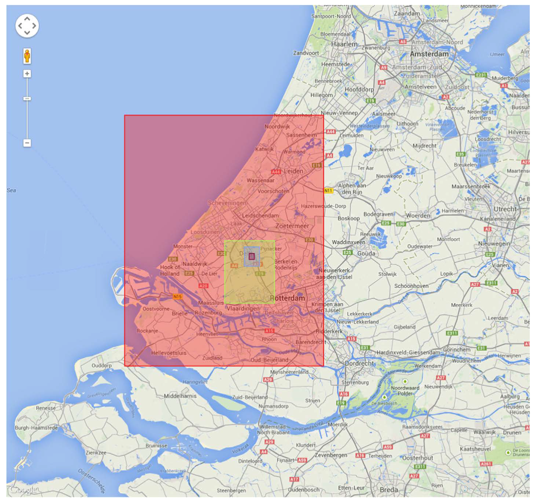
Table 1 we detail the datasets for the scalability test; all of them are subsets of The Netherlands AHN2 dataset, ranging from 20 million to 23 billion. The sample density is 6~10 points per square meter. The experimental datasets have different extents and sizes, and each dataset extends the area covered by a previous smaller dataset, illustrated in
Figure 10.
The hardware configurations for all tests were same as the former benchmark [
19]. For the tests, a HP DL380p Gen8 server with the following details were used: 2-way 8-core Intel Xeon processors, E5-2690 at 2.9 GHz, 128 GB of main memory, and a RHEL 6 operating system. The directly attached storage consists of a 400 GB SSD, 5 TB SAS 15 K rpm in RAID 5 configuration (internal), and 2 × 41 TB SATA 7200 rpm in RAID 5 configuration. The version of Oracle Database is 12c Enterprise Edition Release 12.1.0.1.0-64bit.
4.2. Evaluation of Bulk Points Loading with SFC Encoding
The first step in this subsection is checking how the chunk size of the input point stream affects parallel encoding efficiency. The optimum chunk size established by experiments was used to minimize loading time in the second step.
4.2.1. Parallel LOD Computation and SFC Encoding
This step monitored how long the SFCGen Tool will take for random LOD calculation and 4D SFC key generation (
x/
y/
z/
l) with different chunk sizes on the 20 M dataset. It was done in both serial and parallel modes. All the results are listed in the
Table 2.
The results in
Table 2 show that as the chunk size increases from 5000 to 100,000, the percentage of reduced processing time changes from 17.4 to 29.4%, and the speedup increases from 1.21 to 1.42. This means that the CPU parallelism is better exploited as the chunk size increases. However, although Input/Output overlap in parallel pipelines, the sequential Output still absorbs a large proportion of the total loading time (over 70%). Thus, from this aspect, the speedup is reasonable. The maximum speedup was about 1.45 (141/97 = 1.45).
4.2.2. Bulk Loading with Different-Sized Point Datasets
The bulk loading time recorded the time starting from when the LAS files were read until all points were successfully stored in the Oracle IOT table. Suggested by
Table 2, the chunk size was set to 100,000, and both the sequential and the parallel encoding modes were used in this test (the 2201 M and 23,090 M data are too big and only the parallel mode was used). The coefficients for coordinate transformation were (69,000, 440,000, −100, 0; 100, 100, 100, 1). All the bulk loading results are listed in
Table 3.
Although Hilbert encoding is a little more expensive than Morton encoding, with the help of parallel loading, the differences were significantly shortened (e.g., about 30 s in the 23,090 M dataset). Illustrated in
Table 3, the IOT clustering with Hilbert keys costs significantly less time than clustering with Morton keys (e.g., about 3700 s less for a 23,090 M dataset). This can be attributed to the better clustering capabilities of the Hilbert curve.
4.3. Evaluation of SFC Range Generation and nD Range Query
The first step in this subsection is a check of different range generation configurations on the efficiency of future nD box queries. From the derived optimum configuration, real-case nD box queries were conducted with support from the SFC keys.
4.3.1. Parallel SFC Range Generation
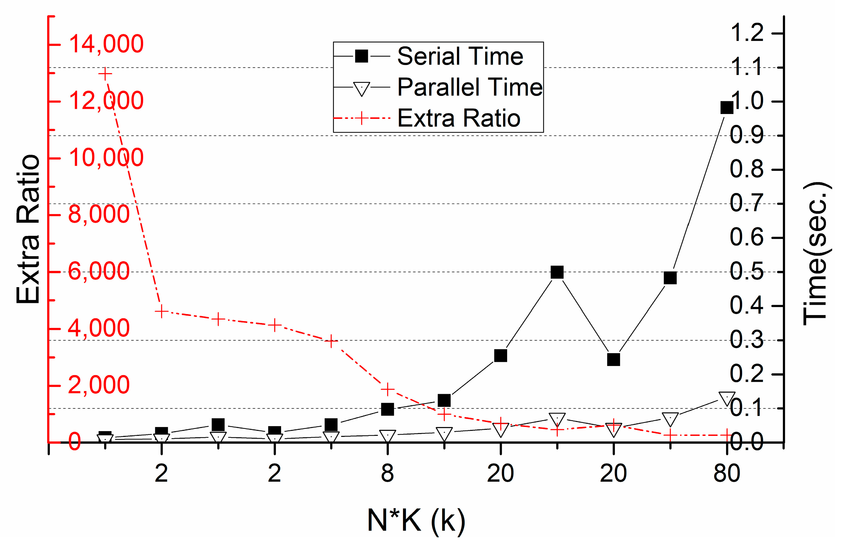
The range generation time monitored how long the SFCQuery Tool spent generating the needed 1D ranges from an nD box as defined by users. The range generation times were obtained with different configurations (N and K). An example parallel range generation command for 4D box input is as follows.
In this command, the total input cell number of a defined 4D box is the product of the side length of a box and the scale coefficient (as specified in
Section 4.2.2) for each dimension, i.e.,
. The returned cell count is the sum of returned range intervals. Usually the returned cell count is much bigger than the total input cell number (shown in
Table 4).
As shown in
Figure 11, the parallel mode decreases generation time considerably as compared to the serial mode, while the speedup increases with a bigger N*K. At the same time, as indicated by the extra ratio between returned cell count and input cell count, the bigger N*K will go down deeper in the 2
n-ary tree traversal and make the returned SFC ranges more precisely approximate the shape of the input 4D box. If given a specific N*K, more returned ranges (i.e., bigger N) are better for later queries.
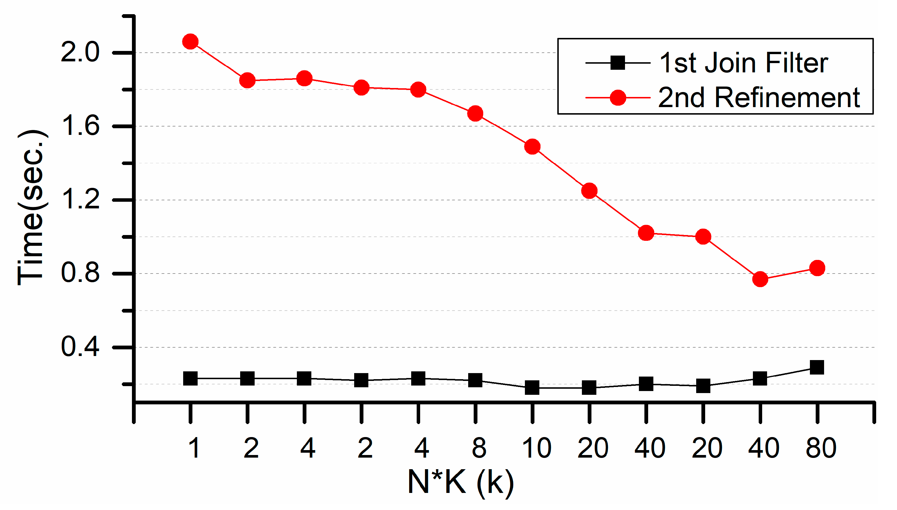
On the 2201 M dataset, a set of real 4D box queries was conducted. As shown in
Table 5 and
Figure 12, a bigger N*K can filter out more points during the 1st join step and a smaller number of points on the left side will make the 2nd refinement much quicker. However, a bigger N*K makes the 1st join step take a much longer time. Therefore, in this test a combination of N = 10,000 and K = 4 gets the smallest query time.
4.3.2. The 4D SFC Query in Real Cases
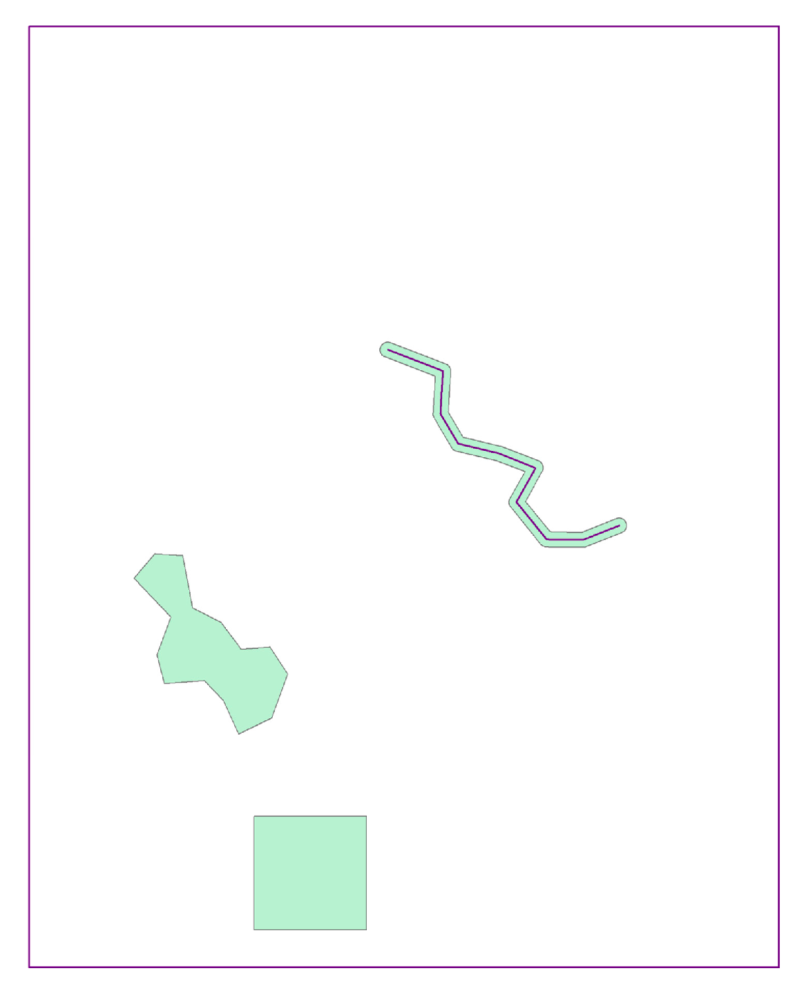
Three geometries were defined for real-case nD SFC queries: Rectangle, Polygon, and Line buffer (shown in
Figure 13). The outer rectangle in
Figure 13 is the bounding box of the 20 M dataset. Different SFC types were also compared (Morton vs Hilbert) on both query time and returned points counts. Suggested by
Figure 13, N and K were set to 10,000 and 4, respectively. Each 4D query filter is listed as follows: (4D_R: 2D_R + −2.0 ≤ VAL_D3 ≤ -1.5 AND 8.0 ≤ VAL_D4 ≤ 9.0; 4D_P: 2D_P + 0.0 ≤ VAL_D3 ≤ 1.0 AND 8.0 ≤ VAL_D4 ≤ 9.0; 4D_B: 2D_B + −3.0 ≤ VAL_D3 ≤ 2.0 AND 8.0 ≤ VAL_D4 ≤ 9.0).
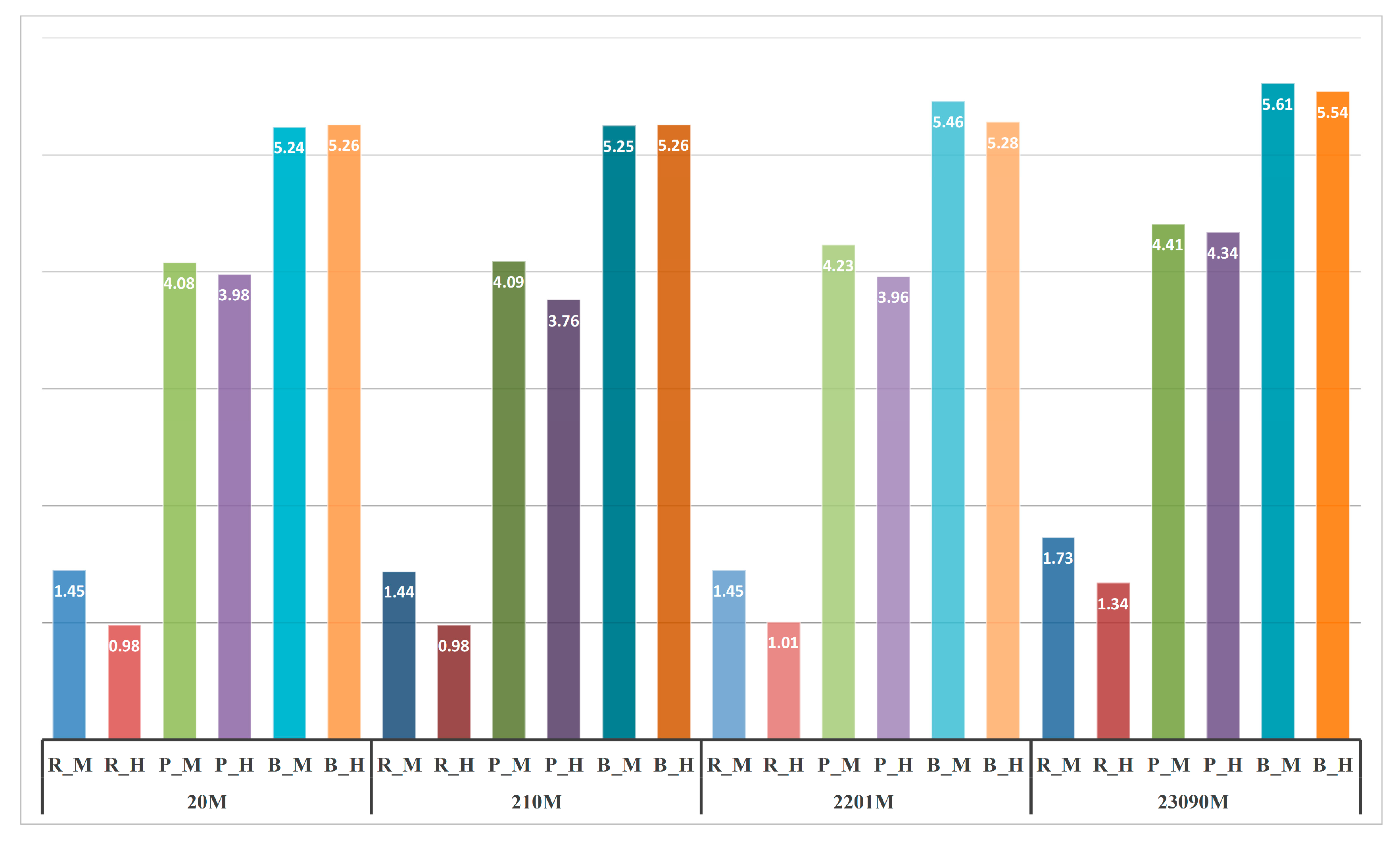
Queries with SFC keys are more scalable over the data size than a pure B-tree filter.
Queries with Hilbert keys are quicker than those with Morton keys (about 0.1 s~0.4 s less time). From same N*K, the derived Hilbert ranges can filter out more points than Morton ranges.
The 1st join filter time is much less than the 2nd refinement time. The 2nd refinement is proportional to the left point count. If the 1st join filter uses more ranges to filter more unrelated points and obtain less-coarse results, then the 2nd refinement will take less time.
4.3.3. The 2D SFC Query in Real Cases
For 2D real-case queries in this 4D organization scheme, two solutions are usually implemented. The first neglects the NULL dimensions and uses the corresponding full dimension range in the SFC space (i.e., 0~2 m). The second uses basic information of actual data about the NULL dimensions and inputs a purposed range that includes the full corresponding range of point datasets (min_value~max_value). Two different solution commands are listed as follows.
The results obtained are listed in
Table 8.
As shown in
Table 8, we can conclude that for 2D query cases, if we cannot specify exact parameters for the NULL dimensions, we can input a reasonable range (min_value~max_value) from information of actual datasets. This is much more efficient than the use of the full dimension range.
5. Discussion
The proposed SFC library can provide complete support for massive points management during the loading, indexing, and later querying. Due to its OOP design, the encapsulated functions of this SFC library can be easily integrated with other frameworks, e.g., [
19]. With the enablement of multithreading, the capability of SFC encoding, decoding, and range generation in the library is greatly accelerated and scales well with input data size.
During the points loading, Hilbert encoding costs a little more time than Morton encoding, but the IOT clustering with Hilbert keys needs much less time than that with Morton keys. Furthermore, the gap of encoding time between Hilbert and Morton is greatly narrowed by parallel implementation. Therefore, the total loading time with Hilbert keys is quicker for massive point datasets. Generally, queries with SFC keys are more scalable over the data size than pure B-tree indexing. Queries with Hilbert keys are quicker than those with Morton keys due to better locality preservation of the Hilbert curve. Therefore, this proves Hilbert keys very suitable for massive points management.
For SFC querying, the total query time depends on the filter capability of generated 1D ranges. The better the quality of the 1D ranges, the much fewer the left points after the 1st join filter will be. The quality of 1D ranges depends on the levels of the 2
n-ary tree traversal, shown in
Section 3.1.2. However, deep traversal still cannot decrease the total query time. Too many 1D ranges will cause the join operations to be extremely expensive. Thus, there exists a balanced level during tree traversal. Due to uneven distribution of input points, some of the generated ranges may filter out no data. Thus, another way to improve the quality of 1D ranges can be done with a statistical histogram of data distribution. If the area represented by one derived range contains no data, this ranges should be excluded from the range collection.
6. Conclusions and Future Work
Since currently no complete and scalable nD Space-Filling Curve library is available for massive point indexing and query retrieval, we propose and implement a generic nD SFC library and apply it to manage massive multiscale LiDAR point clouds. For efficient code reuse, the SFC Library is designed in consideration of object-oriented programming and encapsulates the SFC-related functions, encoding/decoding/query, into abstract classes. It also exploits multicore processor parallelism to accelerate these functions. When integrating this library with massive 4D point cloud management, experimental results show that the proposed nD SFC library provides complete functions for multiscale points management and exhibits robust scalability over massive datasets.
In the near future, the following issues will be investigated:
Real nD geometry query should be supported for future LOD visualization instead of extruded-prism-shape query in 4D cases (2D polygon + 2D attribute filters).
Because SFC keys already contain input coordinate information, coordinate storage in databases might result in redundancy. Key-only storage and decoding in the database will be exploited for higher efficiency.
We will explore true vario-scale/continuous LODs implemented in this proposed method, i.e., importance value per point, instead of by a discrete number of levels.
Our proposed solution can be integrated onto NoSQL databases, e.g., HBase, to support distributed data management with larger datasets (>10 trillion points).
More applications for different point dataset management, e.g., massive trajectory data collected from moving objects, and dynamic true vario-scale data (5D).
Author Contributions
X.G. conceived and designed the algorithm and experiments; X.G. and B.C. implemented the algorithms; X.G. performed the experiments; all authors analyzed the data and experimental results; P.v.O. contributed the high-performance computing infrastructure and gave other financial aid; and X.G. wrote the paper. In addition, we sincerely thank Steve McClure for the language polishing and revising.
Funding
This research was funded by National Key Research and Development Program of China (Grant Number: 2017YFB0503802).
Acknowledgments
Acknowledgements to NUFFIC for Sino-Dutch grant CF 10,570 enabling a one-year visit of Xuefeng Guan to TU Delft. This research is further supported by the Dutch Technology Foundation STW (project number 11185), which is part of The Netherlands Organisation for Scientific Research (NWO), and which is partly funded by the Ministry of Economic Affairs.
Conflicts of Interest
The authors declare no conflict of interest.
Appendix A. Hilbert Encoding/Decoding
Here is the implementation of Hilbert encoding/decoding in the proposed SFC library. Butz proposed an algorithm for generating a Hilbert curve in a byte-oriented manner (the term “byte” is borrowed to represent n bits in an nm-bit SFC key). Butz’s algorithm uses circular shift and exclusive-or operations on bytes, and can generate a Hilbert curve in an arbitrarily high-dimensional space. Lawder suggests some practical improvements to Butz’s algorithm and presents an additional algorithm for inverse mapping from nD values to 1D keys. After clear analysis of Lawder’s paper, two amendments are proposed on it, illustrated as follows.
| n, m | The dimension number n and the curve order m |
| The jth coordinate of the nD point, . |
| The derived m-byte Hilbert key (n bits are called a “byte”), total bits are n*m |
| represents the ith byte in , i.e., ; |
| The derived m-byte Z-order key, total bits are n*m; |
| represents the ith byte in , i.e., ; |
| Principal position in each ith byte of |
| i | Current iteration number of the algorithm, i from 1 to m. |
| parity | The number of bits in a byte which are equal to 1. |
Hilbert Decoding Algorithm (start from 1, repeat i from 1 to m)
| Derive from in |
| (: exclusive-or operation) |
| If then else endif |
| Right circular shift with positions |
| Right circular shift with positions |
| , |
| |
Hilbert Encoding Algorithm (start from 1, repeat i from 1 to m)
| Derive from the input point coordinates, |
| ; |
| ; |
| No shift in ; left circular shift with positions |
| , , …, |
| Derive from in the of |
| Complement in the nth position; if the parity of result byte is odd, complement the result byte in the position |
| No shift in ; left circular shift with positions |
Appendix B. SQLs and Commands Used in the Bulk Loading
The loading operations are listed as follows.
(1) The SQL for the needed temporary Oracle table (D1~D3: coordinates; D4: LOD value; D5: SFC key):
CREATE TABLE AHN_FLAT1_TEMP (VAL_D1 NUMBER, VAL_D2 NUMBER, VAL_D3 NUMBER, VAL_D4 NUMBER, VAL_D5 NUMBER)
TABLESPACE USERS PCTFREE 0 NOLOGGING |
(2) The pipeline command to load the points into the temporary Oracle table:
las2txt -i las_files -stdout -parse xyz -sep comma
| SFCGen -p 0 -s 1 -e 0 -t ct_file -l 10
| sqlldr user/pwd@//localhost:1521/PCTEST direct = true control = ctl_file.ctl data = \’-\’ bad = bad_file.bad log = log_file.log |
(3) The SQL to select all temporary points into the Oracle IOT table:
CREATE TABLE AHN_FLAT1
(VAL_D5, CONSTRAINT AHN_FLAT5_PK PRIMARY KEY (VAL_D5))
ORGANIZATION INDEX
TABLESPACE USERS PCTFREE 0 NOLOGGING
AS SELECT VAL_D5 FROM AHN_FLAT1_TEMP |
Appendix C. SQLs Used in the Two-Step SFC Query
(1) A typical SFCQuery command
| SFCQuery -i d1_min/d1_max/d2_min/d2_max/d3_min/d3_max/d4_min/d4_max -p 1 -s 1 -e 0 -t ct.txt -n 1000 -k 4|sqlldr user/pwd@//localhost:1521/PCTEST direct = true control = 01.ctl data = \’-\’ bad = 01.bad log = 01.log |
(2) The SQL for the 1st SFC Join Filter
CREATE TABLE QUERY_RESULTS_1 AS
SELECT/*+ USE_NL (K S) PARALLEL (8) */ K.*
FROM AHN_FLAT1 K, RANGE_01 S
WHERE K.VAL_D5 BETWEEN S.K1 AND S.K2 |
(3) The SQL for the 2nd Refinement
CREATE TABLE QUERY_RESULTS_1_01
AS (SELECT /* + PARALLEL(8) */ *
FROM TABLE (MDSYS.SDO_POINTINPOLYGON (…..) ///---2D spatial filter
WHERE (VAL_D3 in dim3_range AND VAL_D4 in dim4_range))///---2D Attribute comparison |
References
- Moon, B.; Jagadish, H.V.; Faloutsos, C.; Saltz, J.H. Analysis of the clustering properties of the hilbert space-filling curve. IEEE Trans. Knowl. Data Eng. 2001, 13, 124–141. [Google Scholar] [CrossRef]
- Bader, M. Space-Filling Curves: An Introduction with Applications in Scientific Computing; Springer: Berlin, Germany, 2012; Volume 9. [Google Scholar]
- Nivarti, G.V.; Salehi, M.M.; Bushe, W.K. A mesh partitioning algorithm for preserving spatial locality in arbitrary geometries. J. Comput. Phys. 2015, 281, 352–364. [Google Scholar] [CrossRef]
- Xia, X.; Liang, Q. A gpu-accelerated smoothed particle hydrodynamics (SPH) model for the shallow water equations. Environ. Model. Softw. 2016, 75, 28–43. [Google Scholar] [CrossRef]
- Wang, L.; Ma, Y.; Zomaya, A.Y.; Ranjan, R.; Chen, D. A parallel file system with application-aware data layout policies for massive remote sensing image processing in digital earth. IEEE Trans. Parallel Distrib. Syst. 2015, 26, 1497–1508. [Google Scholar] [CrossRef]
- Huang, Y.-K. Indexing and querying moving objects with uncertain speed and direction in spatiotemporal databases. J. Geogr. Syst. 2014, 16, 139–160. [Google Scholar] [CrossRef]
- Lawder, J.K.; King, P.J. Using space-filling curves for multi-dimensional indexing. In Advances in Databases; Springer: Berlin, Germany, 2000; pp. 20–35. [Google Scholar]
- Zhang, R.; Qi, J.; Stradling, M.; Huang, J. Towards a painless index for spatial objects. ACM Trans. Database Syst. 2014, 39, 1–42. [Google Scholar] [CrossRef]
- Herrero, R.; Ingle, V.K. Space-filling curves applied to compression of ultraspectral images. Signal. Image Video Process. 2015, 9, 1249–1257. [Google Scholar] [CrossRef]
- Nguyen, G.; Franco, P.; Mullot, R.; Ogier, J.M. Mapping high dimensional features onto hilbert curve: Applying to fast image retrieval. In Proceedings of the 21st International Conference on Pattern Recognition (ICPR), Tsukuba, Japan, 11–15 November 2012; pp. 425–428. [Google Scholar]
- van Oosterom, P.; Martinez-Rubi, O.; Ivanova, M.; Horhammer, M.; Geringer, D.; Ravada, S.; Tijssen, T.; Kodde, M.; Gonçalves, R. Massive point cloud data management: Design, implementation and execution of a point cloud benchmark. Comput. Graph. 2015, 49, 92–125. [Google Scholar] [CrossRef]
- Lawder, J.K.; King, P.J.H. Querying multi-dimensional data indexed using the hilbert space-filling curve. SIGMOD Rec. 2001, 30, 19–24. [Google Scholar] [CrossRef]
- Wu, C.-C.; Chang, Y.-I. Quad-splitting algorithm for a window query on a hilbert curve. IET Image Process. 2009, 3, 299–311. [Google Scholar] [CrossRef]
- Jaffer, A. Recurrence for pandimensional space-filling functions. arXiv, 2014; arXiv:1402.1807. [Google Scholar]
- Breinholt, G.; Schierz, C. Algorithm 781: Generating hilbert’s space-filling curve by recursion. ACM Trans. Math. Softw. 1998, 24, 184–189. [Google Scholar] [CrossRef]
- Butz, A.R. Alternative algorithm for hilbert’s space-filling curve. IEEE Trans. Comput. 1971, 100, 424–426. [Google Scholar] [CrossRef]
- Jin, G.; Mellor-Crummey, J. Sfcgen: A framework for efficient generation of multi-dimensional space-filling curves by recursion. ACM Trans. Math. Softw. 2005, 31, 120–148. [Google Scholar] [CrossRef]
- Jaboyedoff, M.; Oppikofer, T.; Abellán, A.; Derron, M.-H.; Loye, A.; Metzger, R.; Pedrazzini, A. Use of lidar in landslide investigations: A review. Nat. Hazards 2012, 61, 5–28. [Google Scholar] [CrossRef]
- van Oosterom, P.; Martinez-Rubi, O.; Tijssen, T.; Gonçalves, R. Realistic benchmarks for point cloud data management systems. In Advances 3D Geoinformation; Springer: Kuala Lumpur, Malaysia, 2015. [Google Scholar]
- Wang, J.; Shan, J. Space filling curve based point clouds index. In Proceedings of the 8th International Conference on GeoComputation, Ann Arbor, MI, USA, 3 August 2005; pp. 551–562. [Google Scholar]
- Guttman, A. R-Trees: A Dynamic Index Structure for Spatial Searching; ACM: New York, NY, USA, 1984; Volume 14. [Google Scholar]
- Kothuri, R.K.V.; Ravada, S.; Abugov, D. Quadtree and r-tree indexes in oracle spatial: A comparison using GIS data. In Proceedings of the 2002 ACM SIGMOD international conference on Management of data, Madison, WI, USA, 3–6 June 2002; pp. 546–557. [Google Scholar]
- van Oosterom, P.; Vijlbrief, T. The spatial location code. In Proceedings of the 7th International Symposium on Spatial Data Handling, Delft, The Netherlands, 12–16 August 1996. [Google Scholar]
- Niemeyer, G. Geohash. Available online: http://geohash.org/ (accessed on 15 August 2018).
- Eldawy, A.; Alarabi, L.; Mokbel, M.F. Spatial partitioning techniques in spatialhadoop. Proc. VLDB Endow. 2015, 8, 1602–1605. [Google Scholar] [CrossRef]
- Guan, X.; Wu, H. Leveraging the power of multi-core platforms for large-scale geospatial data processing: Exemplified by generating DEM from massive LIDAR point clouds. Comput. Geosci. 2010, 36, 1276–1282. [Google Scholar] [CrossRef]
- Kim, W.; Voss, M. Multicore desktop programming with Intel threading building blocks. IEEE Softw. 2011, 28, 23–31. [Google Scholar] [CrossRef]
- Abdelguerfi, M.; Wynne, C.; Cooper, E.; Roy, L. Representation of 3-d elevation in terrain databases using hierarchical triangulated irregular networks: A comparative analysis. Int. J. Geogr. Inf. Sci. 1998, 12, 853–873. [Google Scholar] [CrossRef]
Figure 1.
The illustration of 2D Hilbert curves with different orders.
Figure 1.
The illustration of 2D Hilbert curves with different orders.
Figure 2.
The illustration of dynamic 2D R-tree.
Figure 2.
The illustration of dynamic 2D R-tree.
Figure 3.
A 2D implicit fixed tree labeled with Z-order keys.
Figure 3.
A 2D implicit fixed tree labeled with Z-order keys.
Figure 4.
The abstracted class diagram for SFCLib.
Figure 4.
The abstracted class diagram for SFCLib.
Figure 5.
The relationship between the quadtree node and 1D Hilbert key range.
Figure 5.
The relationship between the quadtree node and 1D Hilbert key range.
Figure 6.
Illustration of the recursive 1D range generation process.
Figure 6.
Illustration of the recursive 1D range generation process.
Figure 7.
The parallel pipeline for bulk SFC encoding.
Figure 7.
The parallel pipeline for bulk SFC encoding.
Figure 8.
The parallel translation from discrete tree nodes to SFC key ranges.
Figure 8.
The parallel translation from discrete tree nodes to SFC key ranges.
Figure 9.
The illustration of streaming random uniform sampling.
Figure 9.
The illustration of streaming random uniform sampling.
Figure 10.
The different experimental datasets displayed on OpenStreetMap.
Figure 10.
The different experimental datasets displayed on OpenStreetMap.
Figure 11.
Parallel SFC range generation for the example 4D query box.
Figure 11.
Parallel SFC range generation for the example 4D query box.
Figure 12.
The query time of two steps with different returned ranges.
Figure 12.
The query time of two steps with different returned ranges.
Figure 13.
Different 2D geometries used in the 4D query cases
Figure 13.
Different 2D geometries used in the 4D query cases
Figure 14.
Total query time over different data sizes in the 4D query cases.
Figure 14.
Total query time over different data sizes in the 4D query cases.
Table 1.
The basic information for the experimental datasets.
Table 1.
The basic information for the experimental datasets.
| Name | Points | Files | Format | Files Size | Area (km2) |
|---|
| 20 M | 20,165,862 | 1 | LAS | 0.4 GB | 1.25 |
| 210 M | 210,631,597 | 17 | LAS | 4 GB | 11.25 |
| 2201 M | 2,201,135,689 | 153 | LAS | 42 GB | 125 |
| 23,090 M | 23,090,482,455 | 1492 | LAS | 440.4 GB | 2000 |
Table 2.
Parallel SFC encoding with different chunk sizes (sec.).
Table 2.
Parallel SFC encoding with different chunk sizes (sec.).
| Chunk Size | Serial Time | Parallel Time | Reduced Time Pct. | Speedup |
|---|
| Input | Encoding | Output | Total Time |
|---|
| 5000 | 14.30 | 18.14 | 96.46 | 128.90 | 106.49 | 17.4% | 1.21 |
| 10,000 | 21.01 | 17.95 | 96.80 | 135.76 | 104.04 | 23.4% | 1.30 |
| 50,000 | 27.39 | 17.45 | 96.71 | 141.55 | 100.28 | 29.2% | 1.41 |
| 100,000 | 27.43 | 17.29 | 96.32 | 141.05 | 99.57 | 29.4% | 1.42 |
Table 3.
Total loading time for different data sizes (sec.).
Table 3.
Total loading time for different data sizes (sec.).
| Data | SFC | Mode | Temp Loading | IOT Clustering | Total Time | Million Pts/sec. |
|---|
| 20 M | M | S | 126.93 | 5.01 | 131.94 | 0.152 |
| H | S | 136.56 | 4.98 | 141.54 | 0.141 |
| M | P | 92.68 | 5.02 | 97.7 | 0.207 |
| H | P | 93.88 | 4.97 | 98.85 | 0.202 |
| 210 M | M | S | 1382.55 | 69.84 | 1452.55 | 0.145 |
| H | S | 1393.06 | 61.78 | 1454.06 | 0.144 |
| M | P | 266.89 | 63.23 | 330.12 | 0.636 |
| H | P | 271.24 | 57.83 | 329.07 | 0.638 |
| 2201 M | M | P | 2094.37 | 1474.20 | 3568.57 | 0.617 |
| H | P | 2114.10 | 1274.37 | 3388.47 | 0.650 |
| 23,090 M | M | P | 22,117.23 | 19,630.07 | 41,747.30 | 0.553 |
| H | P | 22,147.44 | 15,923.96 | 38,071.40 | 0.606 |
Table 4.
The returned range information with different N and K values for this 4D box input (sec.).
Table 4.
The returned range information with different N and K values for this 4D box input (sec.).
| N | K | N*K (*1 k) | Range Num. | Returned Cell Number | Input Cell Number | Extra Ratio | Serial Time | Parallel Time | Speedup |
|---|
| 500 | 2 | 1 | 474 | 145988152983552 | 11250000000 | 12,976.7 | 0.014 | 0.009 | 1.47 |
| 4 | 2 | 490 | 51984203776000 | 11250000000 | 4620.8 | 0.026 | 0.011 | 2.43 |
| 8 | 4 | 475 | 48923216445440 | 11250000000 | 4348.7 | 0.052 | 0.016 | 3.28 |
| 1000 | 2 | 2 | 923 | 46560368918528 | 11250000000 | 4138.7 | 0.029 | 0.011 | 2.58 |
| 4 | 4 | 780 | 40183494868992 | 11250000000 | 3571.9 | 0.052 | 0.017 | 3.13 |
| 8 | 8 | 992 | 21109516795904 | 11250000000 | 1876.4 | 0.097 | 0.022 | 4.34 |
| 5000 | 2 | 10 | 4373 | 11222109454336 | 11250000000 | 997.5 | 0.123 | 0.030 | 4.09 |
| 4 | 20 | 4575 | 7508290043904 | 11250000000 | 667.4 | 0.255 | 0.042 | 6.11 |
| 8 | 40 | 4646 | 5130530185216 | 11250000000 | 456.0 | 0.499 | 0.072 | 6.97 |
| 10,000 | 2 | 20 | 8893 | 6876526411776 | 11250000000 | 611.2 | 0.243 | 0.042 | 5.74 |
| 4 | 40 | 9947 | 2944347791360 | 11250000000 | 261.7 | 0.482 | 0.073 | 6.74 |
| 8 | 80 | 9955 | 2940270893056 | 11250000000 | 261.4 | 0.982 | 0.134 | 7.32 |
Table 5.
4D range query on 2201 M with different returned Hilbert ranges (sec.).
Table 5.
4D range query on 2201 M with different returned Hilbert ranges (sec.).
| N | K | N*K (*1 k) | 1st T | Points | 2nd T | Total T | Points | Ranges |
|---|
| 500 | 2 | 1 | 0.23 | 225,263 | 2.06 | 2.29 | 7559 | 474 |
| 4 | 2 | 0.23 | 217,029 | 1.85 | 2.08 | 7559 | 490 |
| 8 | 4 | 0.23 | 215,527 | 1.86 | 2.09 | 7559 | 475 |
| 1000 | 2 | 2 | 0.22 | 210,221 | 1.81 | 2.03 | 7559 | 923 |
| 4 | 4 | 0.23 | 209,290 | 1.8 | 2.03 | 7559 | 780 |
| 8 | 8 | 0.22 | 203,952 | 1.67 | 1.89 | 7559 | 992 |
| 5000 | 2 | 10 | 0.18 | 168,010 | 1.49 | 1.67 | 7559 | 4373 |
| 4 | 20 | 0.18 | 135,622 | 1.25 | 1.43 | 7559 | 4575 |
| 8 | 40 | 0.2 | 122,767 | 1.02 | 1.22 | 7559 | 4646 |
| 10,000 | 2 | 20 | 0.19 | 117,550 | 1 | 1.19 | 7559 | 8893 |
| 4 | 40 | 0.23 | 85,743 | 0.77 | 1 | 7559 | 9947 |
| 8 | 80 | 0.29 | 85,623 | 0.83 | 1.12 | 7559 | 9955 |
Table 6.
Query time on different data sizes (sec.).
Table 6.
Query time on different data sizes (sec.).
| Data | SFC | Geometry | 1st (Time/Pts) | Total (Time/Pts) | Ranges | Extra Pts (1st/Total) |
|---|
| 20 M | M | 4D_R | 0.17 | 146,220 | 1.45 | 7576 | 7084 | 19.30 |
| 4D_P | 0.25 | 575,545 | 4.08 | 96,628 | 9258 | 5.96 |
| 4D_B | 0.28 | 889,614 | 5.24 | 88,749 | 7078 | 10.02 |
| H | 4D_R | 0.18 | 85,623 | 0.98 | 7560 | 9947 | 11.33 |
| 4D_P | 0.24 | 540,979 | 3.98 | 96,589 | 9315 | 5.60 |
| 4D_B | 0.27 | 859,484 | 5.26 | 88,745 | 6738 | 9.68 |
| 210 M | M | 4D_R | 0.17 | 146,220 | 1.44 | 7567 | 7084 | 19.32 |
| 4D_P | 0.28 | 575,545 | 4.09 | 96,591 | 9258 | 5.96 |
| 4D_B | 0.29 | 889,614 | 5.25 | 88,745 | 7078 | 10.02 |
| H | 4D_R | 0.18 | 85,623 | 0.98 | 7565 | 9947 | 11.32 |
| 4D_P | 0.26 | 540,979 | 3.76 | 96,700 | 9315 | 5.59 |
| 4D_B | 0.32 | 859,484 | 5.26 | 88,729 | 6738 | 9.69 |
| 2201 M | M | 4D_R | 0.22 | 146,220 | 1.45 | 7606 | 7084 | 19.22 |
| 4D_P | 0.28 | 575,545 | 4.23 | 96,634 | 9258 | 5.96 |
| 4D_B | 0.27 | 889,614 | 5.46 | 88,704 | 7078 | 10.03 |
| H | 4D_R | 0.23 | 85,623 | 1.01 | 7559 | 9947 | 11.33 |
| 4D_P | 0.28 | 540,979 | 3.96 | 96,621 | 9315 | 5.60 |
| 4D_B | 0.31 | 859,484 | 5.28 | 88,798 | 6738 | 9.68 |
| 23,090 M | M | 4D_R | 0.41 | 146,220 | 1.73 | 7581 | 7084 | 19.29 |
| 4D_P | 0.58 | 575,545 | 4.41 | 96,582 | 9258 | 5.96 |
| 4D_B | 0.48 | 889,614 | 5.61 | 88,729 | 7078 | 10.03 |
| H | 4D_R | 0.5 | 85,623 | 1.34 | 7539 | 9947 | 11.36 |
| 4D_P | 0.55 | 540,979 | 4.34 | 96,574 | 9315 | 5.60 |
| 4D_B | 0.5 | 859,484 | 5.54 | 88,758 | 6738 | 9.68 |
Table 7.
A comparison of 4D_R query time between Hilbert, Morton, and B-tree (sec.) indices.
Table 7.
A comparison of 4D_R query time between Hilbert, Morton, and B-tree (sec.) indices.
| Data | Morton | Hilbert | B-Tree |
|---|
| 20 M | 1.45 | 0.98 | 0.32 |
| 210 M | 1.44 | 0.98 | 2.1 |
| 2201 M | 1.45 | 1.01 | 119 |
| 23,090 M | 1.73 | 1.34 | 4263 |
Table 8.
2D Rectangle Query time on 20 M points with two solutions (sec.).
Table 8.
2D Rectangle Query time on 20 M points with two solutions (sec.).
| Solution | SFC | 1st (Time/Pts) | Total (Time/Pts) | Ranges | Extra Pts (1st/Total) |
|---|
| 1 | M | 13.98 | 20,165,862 | 124.91 | 322,171 | 305 | 62.59 |
| H | 14.2 | 20,165,862 | 123.45 | 322,171 | 598 | 62.59 |
| 2 | M | 0.21 | 342,454 | 3.57 | 322,171 | 6334 | 1.06 |
| H | 0.23 | 340,047 | 3.37 | 322,171 | 9994 | 1.06 |
© 2018 by the authors. Licensee MDPI, Basel, Switzerland. This article is an open access article distributed under the terms and conditions of the Creative Commons Attribution (CC BY) license (http://creativecommons.org/licenses/by/4.0/).


