Measuring Urban Land Cover Influence on Air Temperature through Multiple Geo-Data—The Case of Milan, Italy

 ,
,  ,
,  , ,
, , 
Abstract
:1. Introduction
2. Materials
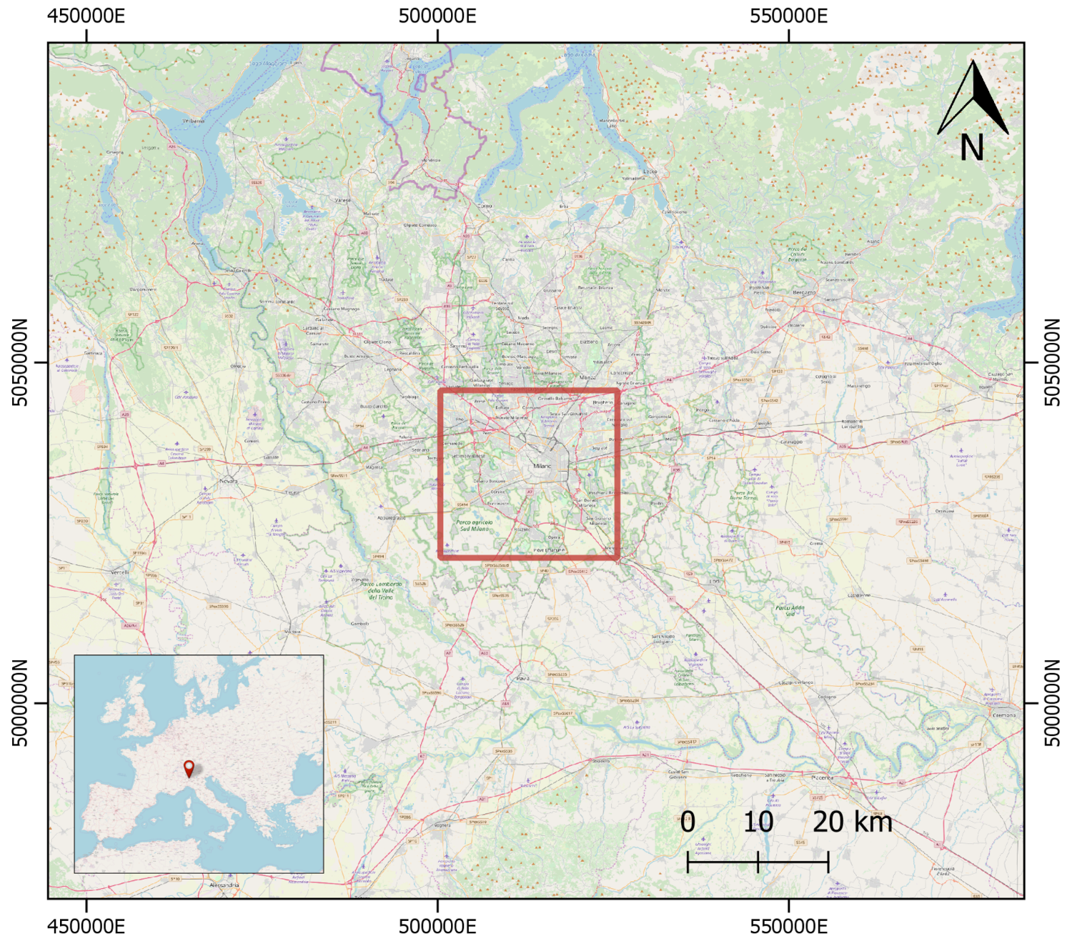
2.1. Study Area
2.2. Data Collection
2.2.1. Satellite Imagery Collection
- Landsat 8: Landsat 8 satellite collects images of the Earth every 16 days in 11 different spectral bands, through two main sensors, an optical sensor (the Operational Land Imager, OLI), and a thermal one (the Thermal Infrared Sensor, TIRS). With the aim of generating LCZ maps exclusively from optical data, thermal, panchromatic, aerosol, and cirrus bands were not considered in this study. Hence, only six bands were considered, which have a spatial resolution of 30 m. Landsat 8 data is freely available for download from GloVis, EarthExplorer, and also LandsatLook Viewer. In this study, data was downloaded through the EarthExplorer platform [31].
- Sentinel-2: The Sentinel-2 satellites acquire, approximately every 5 days, multispectral imagery with 13 bands, but only 10 bands are useful for classification purposes with a spatial resolution of 10 m and 20 m. Sentinel-2 imagery is distributed under a fully open license through the Copernicus Open Access Hub [32] interface. Data access through a dedicated Application Programming Interface (API) is also available.
- RapidEye: The RapidEye satellite constellation provides multispectral images every 5.5 days at nadir. Data are available at 5 m spatial resolution in 5 different spectral bands: Blue, green, red, red-edge, and NIR. RapidEye imagery is distributed under commercial fee by, among the others, Planet Labs Inc. through its Planet Explorer platform [33] API. Free of charge access to the RapidEye archive data API is kindly provided for research groups, with the download limit of 10,000 Km per month.
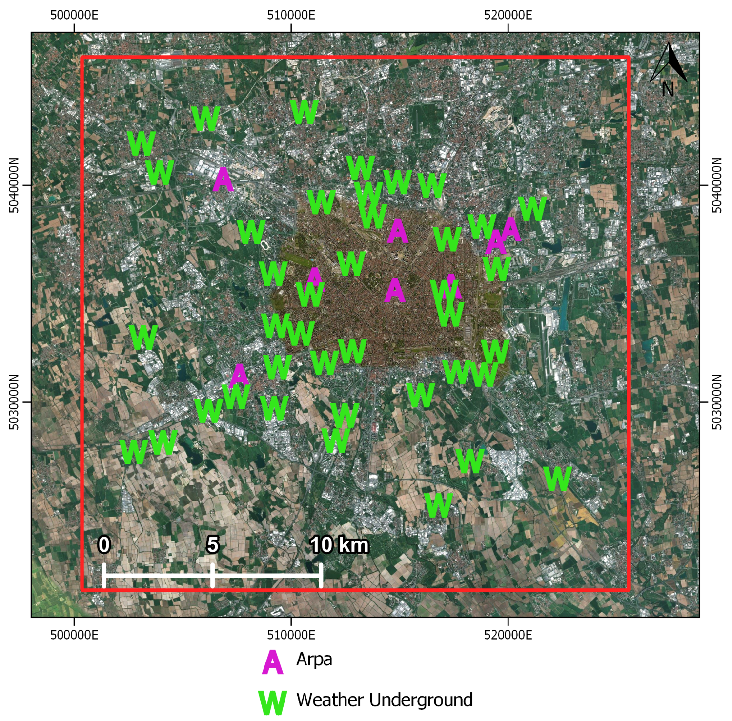
2.2.2. Air Temperature Observations
2.3. Software Tools
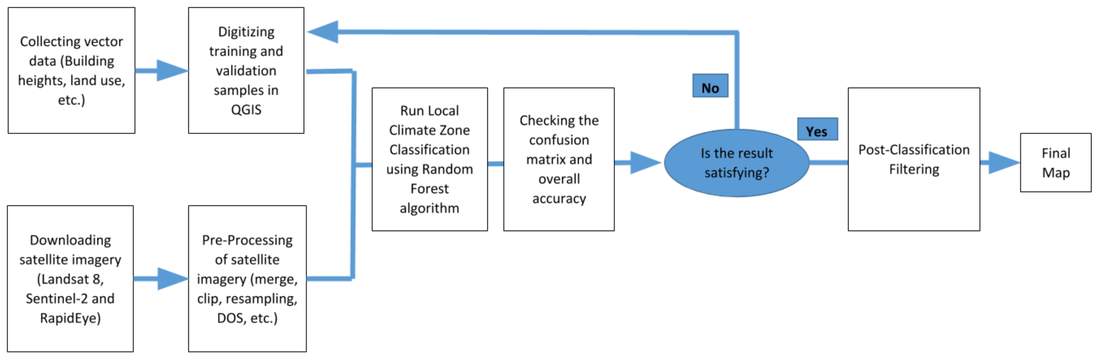
3. Methods
3.1. Data Processing
3.1.1. Satellite Imagery Preprocessing
- Landsat 8: Level-1 data available to users consists of radiometrically and geometrically corrected images. The Level-1 image is presented in units of DNs, which can be easily rescaled to spectral radiance or Top of Atmosphere (TOA) reflectance. In order to obtain real surface reflectance values, band pixels need to be further corrected. The Semi-Automatic Classification Plugin for QGIS [45] was used for such preprocessing.
- Sentinel-2: The Copernicus Open Access Hub provides Sentinel-2 imagery with different level products. In this study Level 1C imagery is used, which is ortho-corrected and with pixel radiometric measurements provided in Top of Atmosphere (ToA) reflectance. Moreover, with the aim of exploiting the complete band set of Sentinel-2 imagery at 10 m spatial resolution, resampling is required. As for Landsat 8 the preprocessing, including atmospheric correction and resampling, was performed through the Semi-Automatic Classification Plugin in QGIS.
- RapidEye: The Planet Explorer platform distributes only ortho-corrected imagery with bands at 5 m spatial resolution. Atmospheric disturbances can be adjusted by exploiting the band reflectance and geometric coefficients available in the metadata file of each tile, in either eXtensible Markup Language (XML) or Javascript Object Notation (JSON) formats, and by applying a Dark Object Subtraction (DOS) procedure [46]. To automate this process, an R script based on the open source Geospatial Data Abstraction Library (GDAL) [47] was created. The script makes also use of the raster R package.
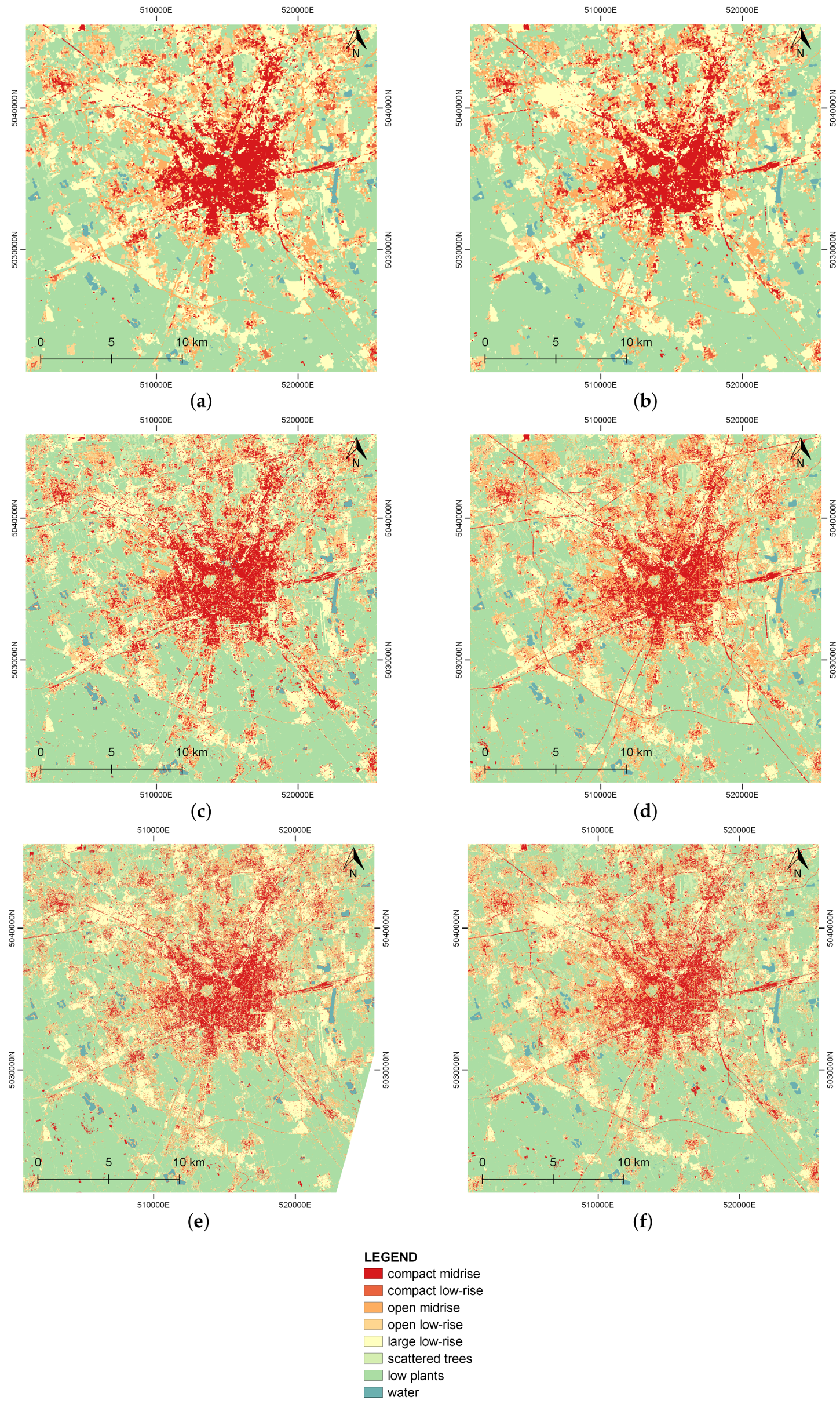
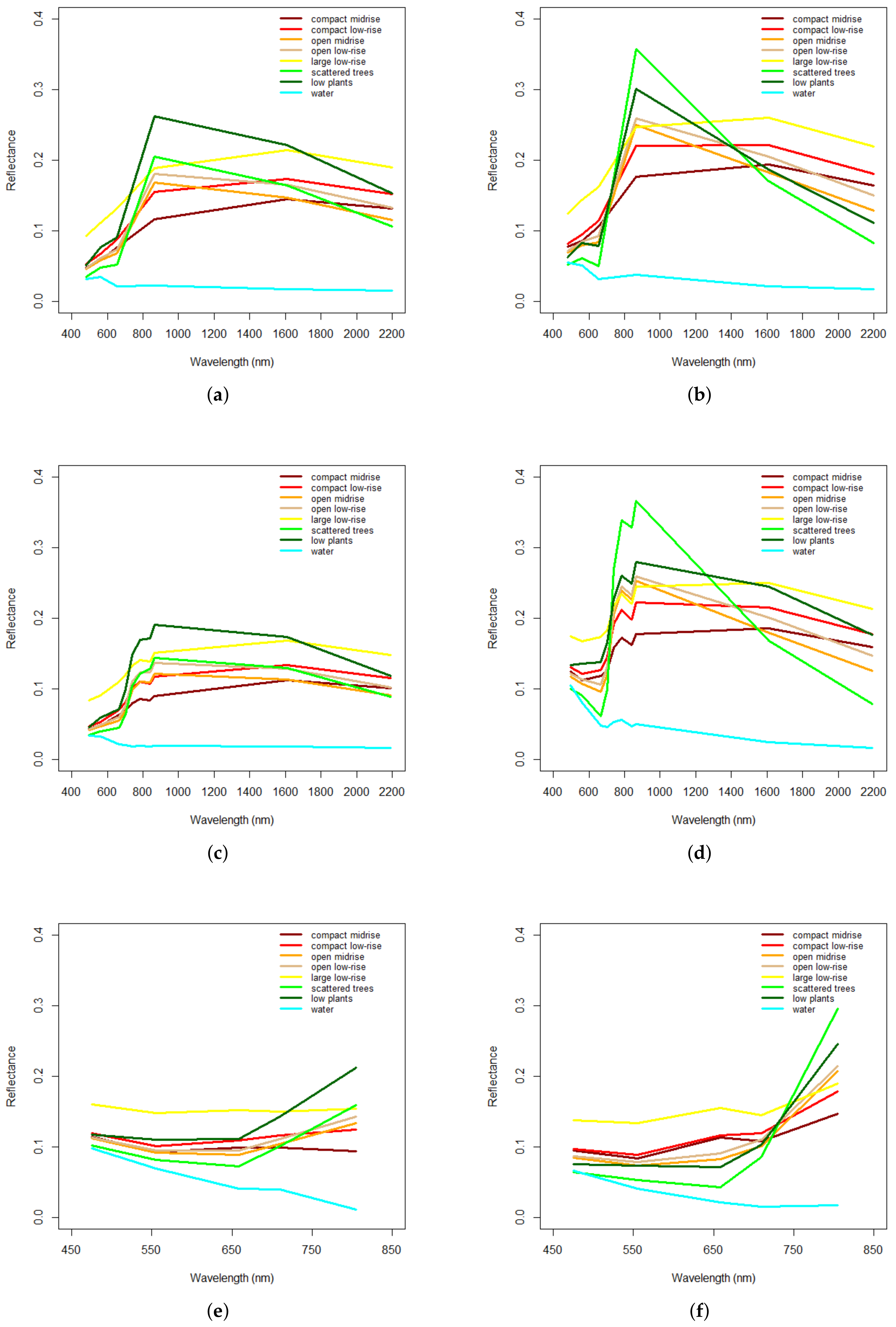
3.1.2. Local Climate Zone (LCZ) mapping
3.1.3. Random Forest (RF) Classification
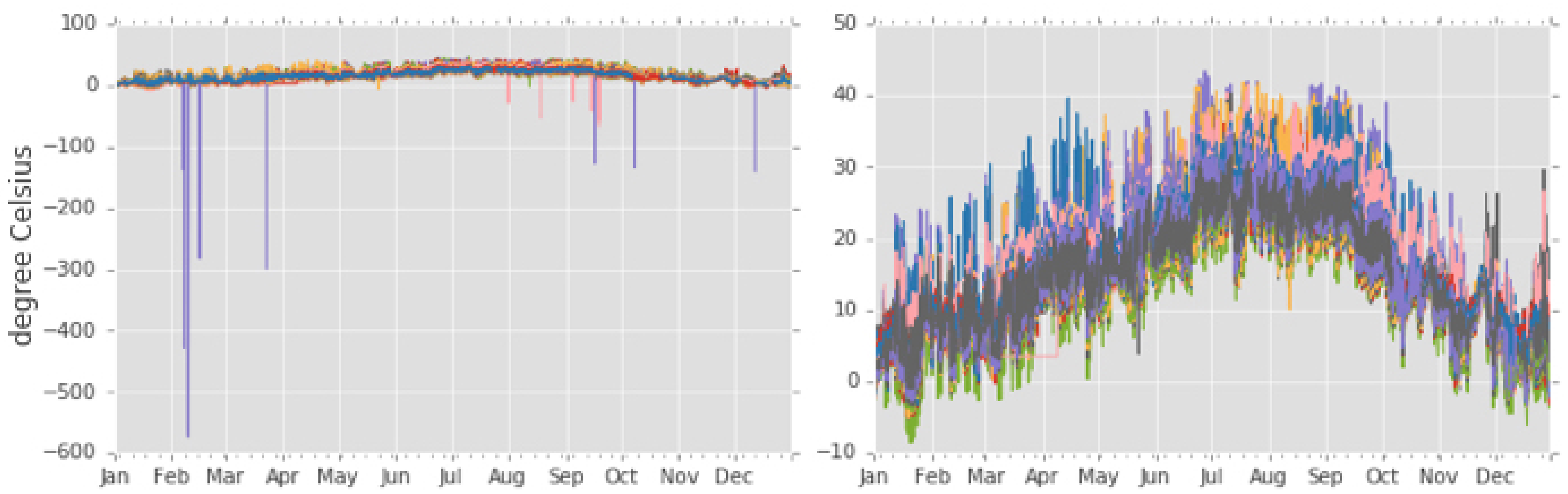
3.1.4. Air Temperature Time Series Adjustment
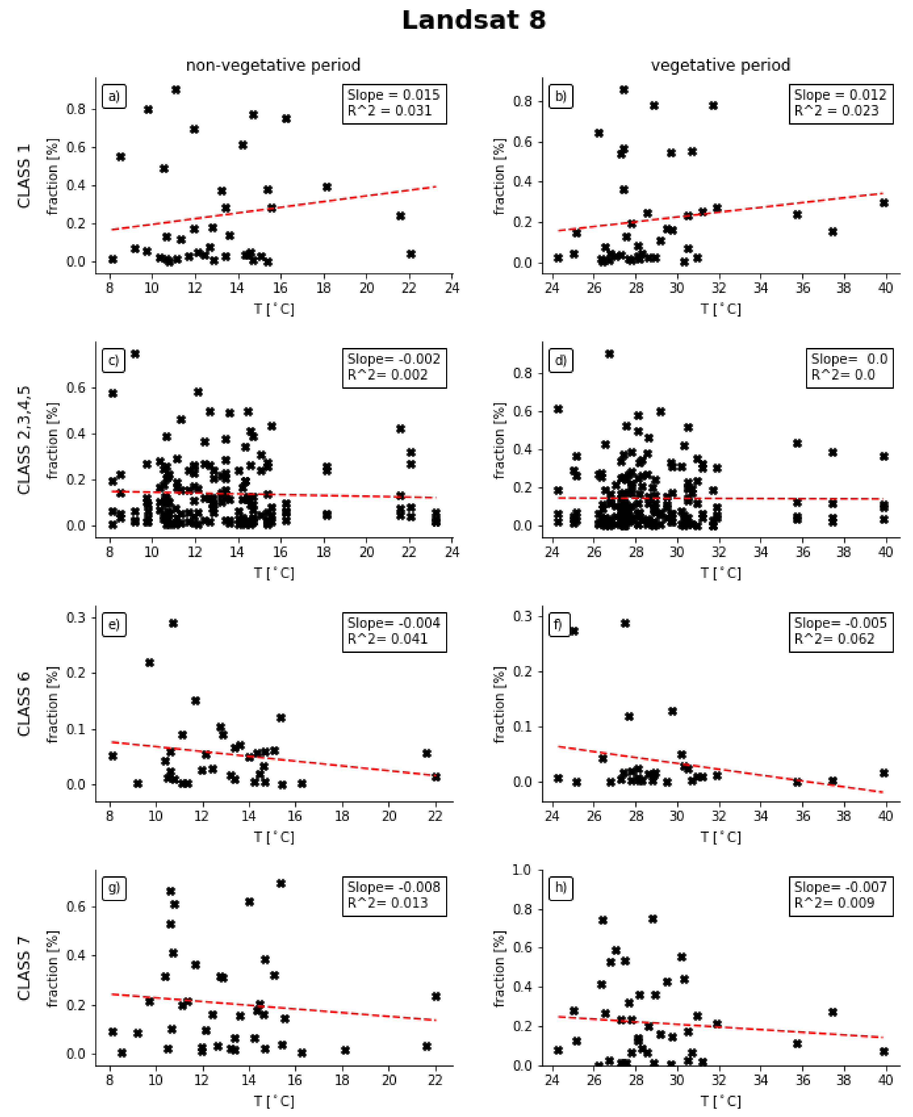
3.2. LCZ and Air Temperature Correlation Analysis
4. Results and Discussion
4.1. LCZ Maps
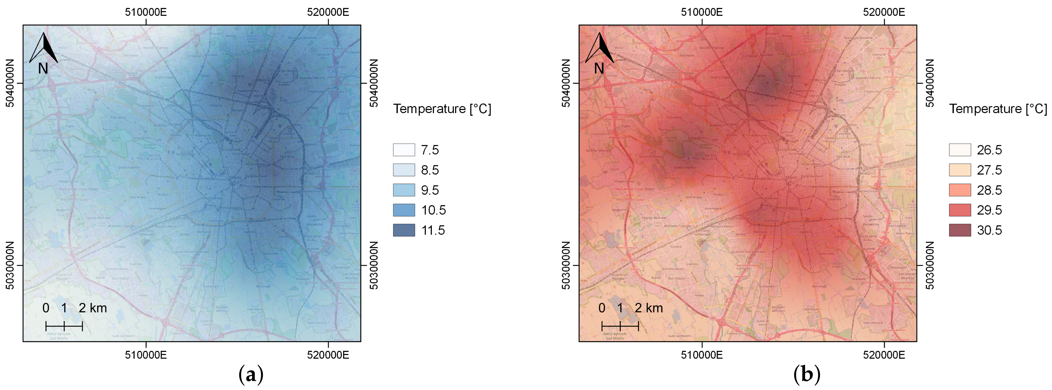
4.2. Air Temperature Patterns in Milan
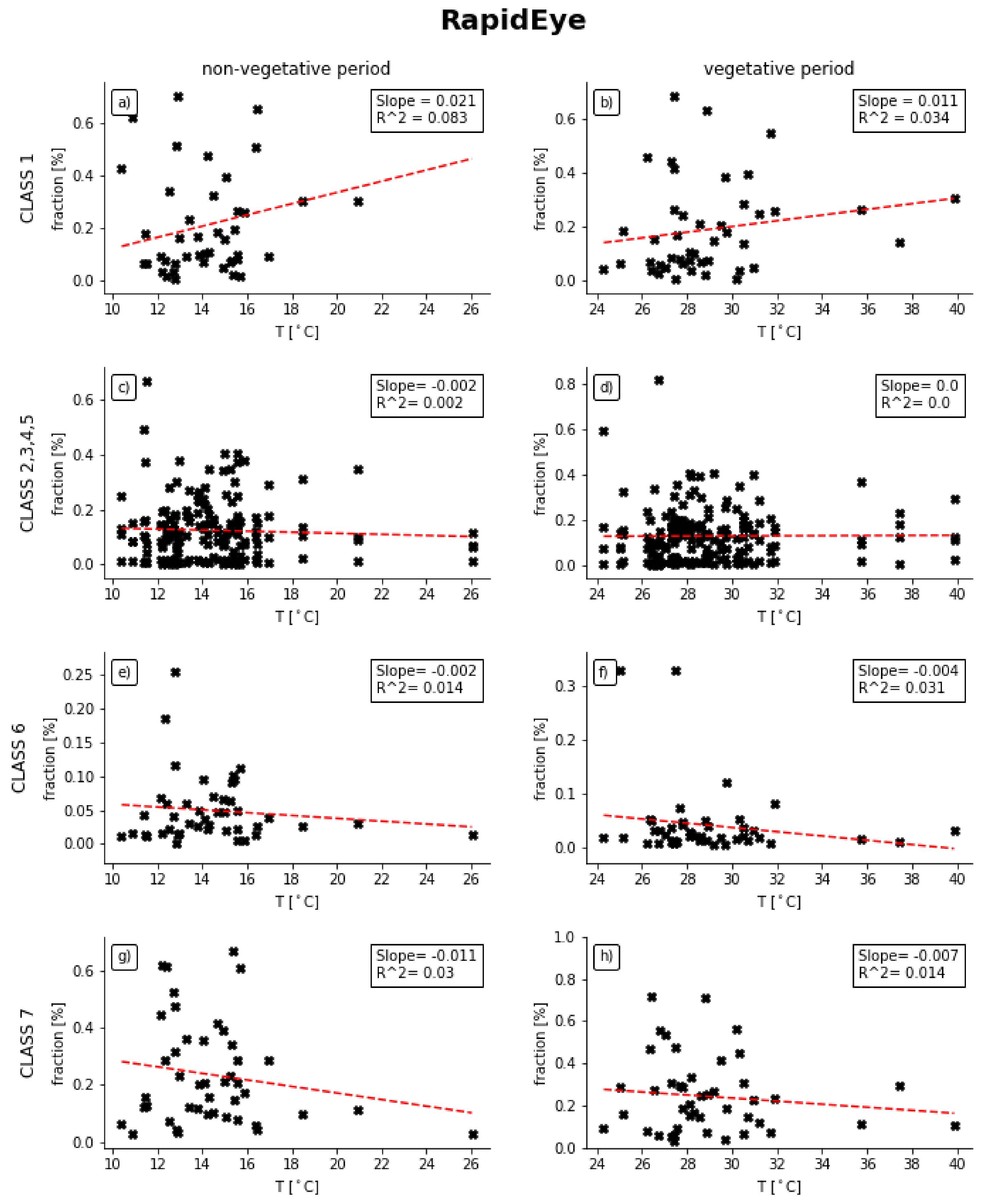
4.3. Correlation Analysis
5. Conclusions
Author Contributions
Funding
Acknowledgments
Conflicts of Interest
References
- Arrhenius, S. On the influence of carbonic acid in the air upon the temperature of the ground. Lond. Edinb. Dublin Phil. Mag. J. Sci. 1896, 41, 237–276. [Google Scholar] [CrossRef]
- Nordhaus, W.D. Managing the Global Commons: The Economics of Climate Change; MIT press: Cambridge, MA, USA, 1994; Volume 31. [Google Scholar]
- Stern, N.; Peters, S.; Bakhshi, V.; Bowen, A.; Cameron, C.; Catovsky, S.; Crane, D.; Cruickshank, S.; Dietz, S.; Edmonson, N.; et al. Stern Review: The Economics of Climate Change; Volume 30, 2006. Available online: http://webarchive.nationalarchives.gov.uk/20100407163608/http://www.hm-treasury.gov.uk/d/SummaryofConclusions.pdf (accessed on 27 October 2018).
- United Nations. World Urbanization Prospects: The 2018 Revision. Available online: https://population.un.org/wup (accessed on 16 September 2018).
- World Bank. Urban Development. Available online: http://www.worldbank.org/en/topic/urbandevelopment/overview (accessed on 16 September 2018).
- UN-Habitat. Cities and Climate Change: Global Report on Human Settlements 2011; UN-Habitat, United Nations Human Settlements Programme: Nairobi, Kenya, 2011. [Google Scholar]
- United Nations. Sustainable Development Goals. Available online: https://www.un.org/sustainabledevelopment (accessed on 16 September 2018).
- Nicholas, S. Growth, Climate and Collaboration: Towards Agreement in Paris 2015. 2014. Available online: http://eprints.lse.ac.uk/64538/1/GrowthClimateandCollaborationStern2014.pdf (accessed on 27 October 2018).
- Faghmous, J.H.; Kumar, V. A big data guide to understanding climate change: The case for theory-guided data science. Big Data 2014, 2, 155–163. [Google Scholar] [CrossRef] [PubMed]
- European Commission. Copernicus. Available online: http://www.copernicus.eu (accessed on 22 September 2018).
- Foody, G.; Fritz, S.; Fonte, C.C.; Bastin, L.; Olteanu-Raimond, A.M.; Mooney, P.; See, L.; Liu, H.Y.; Rodriguez, A.; Minghini, M.; et al. Mapping and the Citizen Sensor. In Mapping and the Citizen Sensor; Foody, G., See, L., Fritz, S., Mooney, P., Olteanu-Raimond, A.M., Fonte, C.C., Antoniou, V., Eds.; Ubiquity Press: London, UK, 2017; pp. 1–12. [Google Scholar] [Green Version]
- Mooney, P.; Minghini, M. A review of OpenStreetMap data. In Mapping and the Citizen Sensor; Foody, G., See, L., Fritz, S., Mooney, P., Olteanu-Raimond, A.M., Fonte, C.C., Antoniou, V., Eds.; Ubiquity Press: London, UK, 2017; pp. 37–57. [Google Scholar]
- Dutta, P.; Aoki, P.M.; Kumar, N.; Mainwaring, A.; Myers, C.; Willett, W.; Woodruff, A. Common sense: Participatory urban sensing using a network of handheld air quality monitors. In Proceedings of the 7th ACM Conference on Embedded Networked Sensor Systems, Berkeley, CA, USA, 4–6 November 2009; pp. 349–350. [Google Scholar]
- Maisonneuve, N.; Stevens, M.; Niessen, M.E.; Steels, L. NoiseTube: Measuring and mapping noise pollution with mobile phones. In Information Technologies in Environmental Engineering; Springer: Berlin, Germany, 2009; pp. 215–228. [Google Scholar] [Green Version]
- Snik, F.; Rietjens, J.H.; Apituley, A.; Volten, H.; Mijling, B.; Di Noia, A.; Heikamp, S.; Heinsbroek, R.C.; Hasekamp, O.P.; Smit, J.M.; et al. Mapping atmospheric aerosols with a citizen science network of smartphone spectropolarimeters. Geophys. Res. Lett. 2014, 41, 7351–7358. [Google Scholar] [CrossRef] [Green Version]
- Oke, T.R. City size and the urban heat island. Atmos. Environ. 1973, 7, 769–779. [Google Scholar] [CrossRef]
- Stewart, I.D.; Oke, T.R. Local climate zones for urban temperature studies. Bull. Am. Meteorol. Soc. 2012, 93, 1879–1900. [Google Scholar] [CrossRef]
- Stewart, I.D.; Oke, T.R.; Krayenhoff, E.S. Evaluation of the ‘local climate zone’scheme using temperature observations and model simulations. Int. J. Climatol. 2014, 34, 1062–1080. [Google Scholar] [CrossRef]
- Long, N.; Gardes, T.; Hidalgo, J.; Masson, V.; Schoetter, R. Influence of the urban morphology on the urban heat island intensity: An approach based on the Local Climate Zone classification. PeerJ 2018, 6, 1–9. [Google Scholar]
- Bechtel, B.; Daneke, C. Classification of local climate zones based on multiple earth observation data. IEEE J. Sel. Top. Appl. Earth Obs. Remote Sens. 2012, 5, 1191. [Google Scholar] [CrossRef]
- WUDAPT. World Urban Database. Available online: http://www.wudapt.org (accessed on 22 September 2018).
- Bechtel, B.; Alexander, P.; Böhner, J.; Ching, J.; Conrad, O.; Feddema, J.; Mills, G.; See, L.; Stewart, I. Mapping local climate zones for a worldwide database of the form and function of cities. ISPRS Int. J. Geo-Inf. 2015, 4, 199–219. [Google Scholar] [CrossRef] [Green Version]
- Dousset, B.; Gourmelon, F. Satellite multi-sensor data analysis of urban surface temperatures and landcover. ISPRS J. Photogramm. Remote Sens. 2003, 58, 43–54. [Google Scholar] [CrossRef]
- Weng, Q.; Lu, D.; Schubring, J. Estimation of land surface temperature—Vegetation abundance relationship for urban heat island studies. Remote Sens. Environ. 2004, 89, 467–483. [Google Scholar] [CrossRef]
- Kawashima, S.; Ishida, T.; Minomura, M.; Miwa, T. Relations between surface temperature and air temperature on a local scale during winter nights. J. Appl. Meteorol. 2000, 39, 1570–1579. [Google Scholar] [CrossRef]
- Mutiibwa, D.; Strachan, S.; Albright, T. Land surface temperature and surface air temperature in complex terrain. IEEE J. Sel. Top. Appl. Earth Obs. Remote Sens. 2015, 8, 4762–4774. [Google Scholar] [CrossRef]
- Nichol, J.E.; Fung, W.Y.; Lam, K.s.; Wong, M.S. Urban heat island diagnosis using ASTER satellite images and ‘in situ’air temperature. Atmos. Res. 2009, 94, 276–284. [Google Scholar] [CrossRef]
- Bacci, P.; Maugeri, M. The urban heat island of Milan. Il Nuovo Cimento C 1992, 15, 417–424. [Google Scholar] [CrossRef]
- Köppen, W. Die Wärmezonen der Erde, nach der Dauer der heissen, gemässigten und kalten Zeit und nach der Wirkung der Wärme auf die organische Welt betrachtet. Meteorol. Zeitsch. 1884, 1, 5–226. [Google Scholar]
- Kopf, S.; Ha-Duong, M.; Hallegatte, S. Using maps of city analogues to display and interpret climate change scenarios and their uncertainty. Nat. Hazards Earth Syst. Sci. 2008, 8, 905–918. [Google Scholar] [CrossRef]
- U.S. Geological Survey. EarthExplorer. Available online: https://earthexplorer.usgs.gov (accessed on 14 September 2018).
- European Commission. Copernicus Open Access Hub. Available online: https://scihub.copernicus.eu (accessed on 14 September 2018).
- Planet Labs Inc. Planet Explorer. Available online: https://www.planet.com/explorer (accessed on 14 September 2018).
- The World in Weather Charts. Available online: http://www1.wetter3.de (accessed on 18 October 2018).
- University of Wyoming—Atmospheric Soundings. Available online: http://weather.uwyo.edu/upperair/sounding (accessed on 18 October 2018).
- TWC Product and Technology LLC. Weather Underground. Available online: https://www.wunderground.com (accessed on 14 September 2018).
- Open Source Geospatial Foundation. QGIS Geographic Information System. Available online: http://qgis.osgeo.org (accessed on 14 September 2018).
- McKinney, W. Pandas: A foundational Python library for data analysis and statistics. In Proceedings of the Python for High Performance and Scientific Computing, Seattle, WA, USA, 18 November 2011; pp. 1–9. [Google Scholar]
- GeoPandas Developers. GeoPandas 0.4.0. Available online: http://geopandas.org (accessed on 14 September 2018).
- Walt, S.v.d.; Colbert, S.C.; Varoquaux, G. The NumPy array: A structure for efficient numerical computation. Comput. Sci. Eng. 2011, 13, 22–30. [Google Scholar] [CrossRef]
- Jones, E.; Oliphant, T.; Peterson, P. SciPy: Open Source Scientific Tools for Python. Available online: http://www.scipy.org (accessed on 14 September 2018).
- Perry, M.T. Rasterstats. Available online: https://pythonhosted.org/rasterstats (accessed on 14 September 2018).
- Hijmans, R.J. Raster: Geographic Data Analysis and Modeling. Available online: https://CRAN.R-project.org/package=raster (accessed on 10 July 2018).
- Liaw, A.; Wiener, M. Classification and Regression by randomForest. R News 2002, 2, 18–22. [Google Scholar]
- Congedo, L. Semi-Automatic Classification Plugin Documentation. Available online: https://semiautomaticclassificationmanual.readthedocs.io (accessed on 14 September 2018).
- Chavez, P.S., Jr. An improved dark-object subtraction technique for atmospheric scattering correction of multispectral data. Remote Sens. Environ. 1988, 24, 459–479. [Google Scholar] [CrossRef]
- GDAL/OGR contributors. GDAL/OGR Geospatial Data Abstraction Software Library. Available online: http://gdal.org (accessed on 14 September 2018).
- Credali, M.; Fasolini, D.; Minnella, L.; Pedrazzini, L.; Peggion, M.; Pezzoli, S. Tools for territorial knowledge and government. In Land Cover Changes in Lombardy Over the Last 50 Years; ERSAF: Milan, Italy, 2011; pp. 17–19. [Google Scholar]
- Regione Lombardia. Database Topografico Regionale (DBTR). Available online: http://www.geoportale.regione.lombardia.it/download-dati (accessed on 14 September 2018).
- Breiman, L. Random forests. Mach. Learn. 2001, 45, 5–32. [Google Scholar] [CrossRef]
- Rodriguez-Galiano, V.F.; Ghimire, B.; Rogan, J.; Chica-Olmo, M.; Rigol-Sanchez, J.P. An assessment of the effectiveness of a random forest classifier for land-cover classification. ISPRS J. Photogram. Remote Sens. 2012, 67, 93–104. [Google Scholar] [CrossRef]
- Congalton, R.G.; Green, K. Assessing the Accuracy of Remotely Sensed Data: Principles And Practices; CRC Press: Boca Raton, FL, USA, 2008. [Google Scholar]
- Rozenstein, O.; Karnieli, A. Comparison of methods for land-use classification incorporating remote sensing and GIS inputs. Appli. Geogr. 2011, 31, 533–544. [Google Scholar] [CrossRef]
- Box, G.E.; Jenkins, G.M.; Reinsel, G.C.; Ljung, G.M. Time Series Analysis: Forecasting and Control; John Wiley & Sons: Hoboken, NJ, USA, 2015. [Google Scholar]
- ISPRA. Variazioni E Tendenze Degli Estremi Di Temperatura E Precipitazione in Italia. 2013. Available online: https://tinyurl.com/ycay4jaj (accessed on 14 September 2018).
- Sapkota, B.B.; Liang, L. A multistep approach to classify full canopy and leafless trees in bottomland hardwoods using very high-resolution imagery. J. Sustain. For. 2018, 37, 339–356. [Google Scholar] [CrossRef]
- Cressie, N. Spatial prediction and ordinary kriging. Math. Geol. 1988, 20, 405–421. [Google Scholar] [CrossRef]
- Gräler, B.; Pebesma, E.; Heuvelink, G. Spatio-Temporal Interpolation using gstat. R J. 2016, 8, 204–218. [Google Scholar]
- Arnfield, A.J. Two decades of urban climate research: A review of turbulence, exchanges of energy and water, and the urban heat island. Int. J. Climatol. 2003, 23, 1–26. [Google Scholar] [CrossRef]
- De Groof, H. Remarks at the Closing Plenary of the INSPIRE 2018 Conference. In Proceedings of the INSPIRE 2018 Conference, Antwerp, Belgium, 18–21 September 2018. [Google Scholar]
- Brovelli, M.A.; Minghini, M.; Moreno-Sanchez, R.; Oliveira, R. Free and open source software for geospatial applications (FOSS4G) to support Future Earth. Int. J. Digit. Earth 2017, 10, 386–404. [Google Scholar] [CrossRef]


| Satellite | Acquisition Date and Time | |
|---|---|---|
| Non-Vegetative | Vegetative | |
| Landsat 8 | 18-03-2016 10:10 a.m. | 22-06-2016 10:10 a.m. |
| Sentinel-2 | 13-01-2016 10:20 a.m. | 22-05-2016 10:20 a.m. |
| RapidEye | 18-03-2016 11:14 a.m. | 22-06-2016 10:46 a.m. |
| Acquisition Date | Synoptic Parameters |
|---|---|
| 13-01-2016 | Geopotential height 500 hPa: 5450 m (↓) Wind Direction 500 hPa: 315 deg Advection 850 hPa: Cold Thermodinamical Profile: Stable |
| 18-03-2016 | Geopotential height 500 hPa: 5560 m (↔) Wind Direction 500 hPa: 105 deg Advection 850 hPa: No advection Thermodinamical Profile: Stable |
| 22-05-2016 | Geopotential height 500 hPa: 5740 m (↑) Wind Direction 500 hPa: 200 deg Advection 850 hPa: Warm Thermodinamical Profile: Stable |
| 22-06-2016 | Geopotential height 500 hPa: 5890 m (↑) Wind Direction 500 hPa: 20 deg Advection 850 hPa: Warm Thermodinamical Profile: Stable |
| Class ID | Class Name | Description |
|---|---|---|
| 1 | Compact midrise | Dense mix of midrise buildings (3–9 stories). Few or no trees. Land cover mostly paved. Stone, brick, tile, and concrete construction material. |
| 2 | Compact low-rise | Dense mix of low-rise building (1–3 stories). Few or no trees. Land cover mostly paved. Stone, brick, tile, and concrete construction material. |
| 3 | Open midrise | Open arrangement of midrise buildings (3–9 stories). Abundance of pervious land cover (low plants, scattered trees). Concrete, steel, stone, and glass construction materials. |
| 4 | Open low-rise | Open arrangement of low-rise buildings (1–3 stories). Abundance of pervious land cover (low plants, scattered trees). Wood, brick, stone, tile, and concrete construction materials. |
| 5 | Large low-rise | Open arrangement of large low-rise buildings (1–3 stories). Few or no trees. Land cover mostly paved. Steel, concrete, metal, and stone construction materials. |
| 6 | Scattered trees | Lightly wooded landscape of deciduous and/or evergreen trees. Land cover mostly pervious (low plants). Zone function is natural forest, tree cultivation, or urban park. |
| 7 | Low plants | Featureless landscape of glass or herbaceous plants/crops. Few or no trees. Zone function is natural grassland, agriculture, or urban park. |
| 8 | Water | Large, open water bodies such as seas or lake, or small bodies such as rivers, reservoirs, and lagoons. |
| Satellite | Period | |
|---|---|---|
| Non-Vegetative | Vegetative | |
| Landsat 8 | 81.43 | 80.56 |
| Sentinel-2 | 75.57 | 78.70 |
| RapidEye | 71.79 | 71.61 |
| Satellite | Period | Majority Class ID | Number of Buffers | Median C | Standard Deviation C |
|---|---|---|---|---|---|
| Landsat 8 | Non-Vegetative | 1 | 13 | 10.59 | 1.2 |
| 2,3,4,5 | 23 | 9.60 | 1.5 | ||
| 6 | 0 | / | / | ||
| 7 | 12 | 8.98 | 0.8 | ||
| Landsat 8 | Vegetative | 1 | 11 | 21.97 | 0.9 |
| 2,3,4,5 | 23 | 21.46 | 1.1 | ||
| 6 | 0 | / | / | ||
| 7 | 14 | 20.84 | 0.7 | ||
| Sentinel-2 | Non-Vegetative | 1 | 18 | 5.46 | 1.2 |
| 2,3,4,5 | 14 | 4.68 | 1.5 | ||
| 6 | 0 | / | / | ||
| 7 | 16 | 3.93 | 0.9 | ||
| Sentinel-2 | Vegetative | 1 | 12 | 19.15 | 1 |
| 2,3,4,5 | 21 | 18.58 | 1.1 | ||
| 6 | 2 | 16.69 | / | ||
| 7 | 13 | 18.08 | 0.6 | ||
| RapidEye | Non-Vegetative | 1 | 12 | 11.02 | 1.7 |
| 2,3,4,5 | 18 | 9.97 | 0.9 | ||
| 6 | 0 | / | / | ||
| 7 | 18 | 9.02 | 1.1 | ||
| RapidEye | Vegetative | 1 | 13 | 21.97 | 0.9 |
| 2,3,4,5 | 17 | 21.30 | 1.2 | ||
| 6 | 1 | 19.53 | / | ||
| 7 | 17 | 20.90 | 0.8 |
© 2018 by the authors. Licensee MDPI, Basel, Switzerland. This article is an open access article distributed under the terms and conditions of the Creative Commons Attribution (CC BY) license (http://creativecommons.org/licenses/by/4.0/).
Share and Cite
Oxoli, D.; Ronchetti, G.; Minghini, M.; Molinari, M.E.; Lotfian, M.; Sona, G.; Brovelli, M.A. Measuring Urban Land Cover Influence on Air Temperature through Multiple Geo-Data—The Case of Milan, Italy. ISPRS Int. J. Geo-Inf. 2018, 7, 421. https://0-doi-org.brum.beds.ac.uk/10.3390/ijgi7110421
Oxoli D, Ronchetti G, Minghini M, Molinari ME, Lotfian M, Sona G, Brovelli MA. Measuring Urban Land Cover Influence on Air Temperature through Multiple Geo-Data—The Case of Milan, Italy. ISPRS International Journal of Geo-Information. 2018; 7(11):421. https://0-doi-org.brum.beds.ac.uk/10.3390/ijgi7110421
Chicago/Turabian StyleOxoli, Daniele, Giulia Ronchetti, Marco Minghini, Monia Elisa Molinari, Maryam Lotfian, Giovanna Sona, and Maria Antonia Brovelli. 2018. "Measuring Urban Land Cover Influence on Air Temperature through Multiple Geo-Data—The Case of Milan, Italy" ISPRS International Journal of Geo-Information 7, no. 11: 421. https://0-doi-org.brum.beds.ac.uk/10.3390/ijgi7110421