Semantic Geometric Modelling of Unstructured Indoor Point Cloud


Department of Land Surveying and Geo-Informatics, The Hong Kong Polytechnic University, Hung Hom, Kowloon, Hong Kong, China
*
Author to whom correspondence should be addressed.
ISPRS Int. J. Geo-Inf. 2019, 8(1), 9; https://0-doi-org.brum.beds.ac.uk/10.3390/ijgi8010009
Submission received: 24 October 2018
/
Revised: 24 November 2018
/
Accepted: 17 December 2018
/
Published: 27 December 2018
Abstract
:A method capable of automatically reconstructing 3D building models with semantic information from the unstructured 3D point cloud of indoor scenes is presented in this paper. This method has three main steps: 3D segmentation using a new hybrid algorithm, room layout reconstruction, and wall-surface object reconstruction by using an enriched approach. Unlike existing methods, this method aims to detect, cluster, and model complex structures without having prior scanner or trajectory information. In addition, this method enables the accurate detection of wall-surface “defacements”, such as windows, doors, and virtual openings. In addition to the detection of wall-surface apertures, the detection of closed objects, such as doors, is also possible. Hence, for the first time, the whole 3D modelling process of the indoor scene from a backpack laser scanner (BLS) dataset was achieved and is recorded for the first time. This novel method was validated using both synthetic data and real data acquired by a developed BLS system for indoor scenes. Evaluating our approach on synthetic datasets achieved a precision of around 94% and a recall of around 97%, while for BLS datasets our approach achieved a precision of around 95% and a recall of around 89%. The results reveal this novel method to be robust and accurate for 3D indoor modelling.
1. Introduction
Recently, 3D building modelling has attracted the attention of several scholars in disciplines, such as photogrammetry [1,2,3], geo-informatics [4,5,6], and computer graphics [7,8,9,10]. Indoor scene reconstruction has been found to be a more challenging task than that of the outdoor scenes, as such areas tend to have high clutter. Indoor models have a valuable role in many applications, such as planning and building construction monitoring, localization and navigation services in public buildings, virtual models for historical and cultural sites, city planning decision making, and accelerating the construction process using a digitized model [6,11]. Three major reasons have been identified as driving forces behind 3D building modelling: The necessity to (a) reduce the data used, (b) extract and reconstruct objects from unstructured 3D point clouds, and (c) fit semantics to buildings [12].
Indoor building modelling in 3D space is necessary for different applications, hence fast scanning devices are manufactured for creating a point cloud, which is the source to start modelling. Besides, various indoor models, such as geometric, grid, topology, semantic, and hybrid models have been proposed to deal with these data [13]. Despite these different models, 3D modelling from a point cloud is still time-consuming, because of the manual involvement [14].
Determining structural elements (i.e., wall, ceiling, and floor) or wall-surface features (i.e., window, door, and virtual openings) from indoor environments despite visual interruptions poses specific challenges, such as clutter that depends on the environment of the scene (e.g., office, apartment) and occlusion that is due to furniture that covers both wall and window sections. A further challenge is the complexity of room layouts: Some layouts follow regular shapes, but others do not.
The complexity of indoor environments poses individually related considerations which have been tackled using different approaches. One approach called Manhattan world assumption involves the detection of orthogonal room clusters only [15,16]. That assumption was released as most manmade objects, during construction, follow a natural Cartesian reference system [17]. Another approach involved the modelling of complex room layouts, but that approach depended mainly on the scanner position, with at least one scan per room [8,14]. Another approach can only deal with one room with complex structure [18], or modelling the outer boundary of complex structure regardless of the inner structures, such as ventilation holes or inaccessible rooms [19].
The corresponding focus presented in the proposed approach involves the 3D modelling of complex indoor scenes, dependent only on the availability of spatial information obtained from a backpack laser scanner (BLS) system and without any previously collected information. From a 3D unstructured point cloud, the proposed approach is able to automatically generate a 2D segmented floor plan without any assumptions regarding wall partition directions and can detect wall-surface objects (opened and closed). This method uses both data-driven approaches that utilize complex algorithms without prior knowledge of the scene, and model-driven approaches that utilize predefined primitives to construct the model. Although it is based on previous work, the work presented in this paper includes the following unique aspects:
- A novel framework for the automatic reconstruction of indoor building models from BLS, which provides a realistic construction with semantic information. Only the 3D point cloud is needed for the processing;
- A new hybrid segmentation approach that enhances the segmentation process of the point cloud;
- An adjustment of patch boundaries using the wall segments which enhance the geometry of structural elements;
- An enriched wall-surface object detection that can detect not only open objects, but closed objects as well.
The remainder of this paper is organized as follows: We present related work that has been conducted using existing approaches for modelling indoor structures, and the novel methodology used for the framework developed in the proposed approach is presented, together with an analysis of each step taken, experiments conducted, and further explanatory discussion. Conclusions are given together with associated recommendations for future work.
2. Related Work
Modelling indoor scenes have been an area of research focus in past decades, with the aim of developing and satisfying the need for further applications. As presented by Reference [13], there are currently five spatial data models available for modelling indoor structures. The first is geometric modelling, which uses precise coordinates to geometrically describe the spatial structure and its components. The second model is a grid model which uses regular or irregular (Voronoi diagram) grid size for representing the interior space. When the interest is more regarding interior path planning, modelling procedures arrive at the third model, which is a topological model. The fourth model is a semantic model which is concerned with defining all different types of indoor spatial objects. Due to some defacements of such models, the hybrid model is introduced to tackle these limitations. In general, all the existing modelling methods used in relation to indoor structures follow one of the following two approaches: Manhattan world assumption, or previous scanner knowledge. These approaches were applied, each to a different dataset: Terrestrial laser scanner (TLS), panorama RGB image point cloud, RGB-Depth images, and mobile laser scanner (MLS). The existing indoor modelling research is described in the following section, based on two different approaches, including a discussion of their limitations.
2.1. Manhattan World Assumption
This assumption was released because most manmade objects, during construction, follow a natural Cartesian reference system [17]. Most of the existing work follows that simplification assumption when modelling complex indoor structures. Xiao and Furukawa [1] built a texturing 3D model for a museum from images and a laser scanner dataset. The inverse constructive solid geometry (CSG) method was used for modelling the indoor space of the museum, which assumes that the outdoor space taken over by the wall is filled in. The Manhattan world assumption was used with the alignment of a vertical direction with gravity. CSG was conducted in 2D space for slices taken in 3D space, then different patches were combined to produce a 3D CSG model. Cabral and Furukawa [2] used a set of panoramic images to generate a 3D model with the assumption of Manhattan world. Structure from motion (SfM) and multi-view stereo (MVS) algorithms were used to enable camera pose estimation and also recover points in 3D space. The reconstructed point cloud was processed for a 2D floor plane using the shortest path algorithm. Ikehata et al. [16] applied an approach for the modelling of an indoor scene from panorama RGBD (red green blue depth) image datasets. The k-medoids algorithm was applied to the point cloud datasets, depending on the free space pixel evidence, followed by the construction of room boundaries using a shortest-path based algorithm. RANSAC was applied to each room separately to detect vertical walls, while the floor and ceiling were estimated as horizontal planes. The constructed room boundaries were modified using robust principal component analysis and Markov random field, depending on the generated planar depth map. This method was applicable for the detection of structural elements of different heights, but nonetheless was successful in working with assumed Manhattan world directions. Murali et al. [15] presented an RGB-Depths dataset modelling approach. They applied RANSAC for the plane detection of vertical walls, and other planes were extracted by the orientation of the dataset parallel to the real world. The constructed walls were intersected, and cuboids generated, followed by the cutting and implementation of the wall graph to minimize such cuboids in individual rooms. All openings were found using a connected component labelling algorithm. This technique was not sufficient to detect all openings due to two factors: The noise in the RGBD dataset, and the assumption of the simplified room layout with perpendicular sides.
2.2. Scanner Prior Knowledge
In contrast to the Manhattan world assumption approach where some bellringings do not follow that rule, researchers have used scanner position or trajectory to help to model complex structural elements or detect wall-surface objects. Ochmann et al. [14] proposed an automatic method to enable the construction of indoor scenes from a terrestrial laser scanner dataset with multiple scans—at least one scanner per room. Point segmentation was achieved based on the scanning point information for each scan of different room segments. RANSAC was then implemented to detect wall candidates. For further wall candidate segmentation, any two walls with a predetermined threshold were considered for one wall and the centerline wall was used for modelling. The optimal layout of each room was considered as a labelling problem, and therefore labelling followed an energy minimization approach. Wall-surface objects were then detected by estimating the intersection points between the reconstructed walls and simulated laser rays from the scan positions, and the measured points. These objects were classified as a door, window, and virtual openings using a six-dimensional feature vector. The core of that work depended mainly on the relative position of the scanner and scanned points, which may not be found in other scan devices. Wang et al. [9] applied an automatic method for modelling structural elements from MLS datasets. First of all, the raw datasets were filtered using statistical analysis and morphological filters, and principal component analysis (PCA) was then used to consolidate the wall points based on the threshold and differences of the point’s normal direction and vertical direction. To capture a more precise detection, the wall points were consolidated by projecting all 3D points into 2D space from the bottom to the top. If a voxel had no points in the Z direction within 1.0 m, all points would not be projected in the 2D plan. The projected 2D points were processed using RANSAC followed by 1D mean shift clustering to define the main wall segments. The wall segments were decomposed into cells, labelled using energy function and graph cut algorithm as outer wall cells and inner wall cells. The latter was based on the use of line-of-sight information for each cell identified by the scanner position from the trajectory. The doorway was detected based on the intersection of the trajectory, and detected holes using an alpha shape algorithm. Room recognition and segmentation were applied using a Markov transition matrix and the k-medoids algorithm. The proposed approach could construct a model with structural elements and opened doors only and failed to detect different wall-surface objects (i.e., closed doors, windows, or virtual openings). Michailidis and Pajarola [10] presented an approach for the construction of wall-surface objects, such as windows and doors using an optimized Bayesian graph-cut applied on a terrestrial laser scanner dataset collected from several scans for one wall. This technique involved wall-surface segmentation and was applied to detect the main wall structure. Each separated wall segment was processed using an alpha shape algorithm to detect its boundaries. Linear features were detected using RANSAC, and these lines were clustered for more robustness. In addition to these lines, a cell complex creation was produced using a 2D grid of the wall. Occluded parts from furniture were also recovered and labelled. Graph cut optimization was implemented based on different weighted values to recover the opening parts, such as different openings with complex shapes, but related only to buildings also including planar and vertical walls. A further vital consideration is the relative position of the scanner and the scanned walls.
From the literature above and as concluded in Table 1, it is clear that most of the approaches described have limitations as regards the generation of as-built indoor models, particularly when such models have complex structural elements and are adorned or enhanced by wall-surface objects. Such approaches were constructed based on the use of the Manhattan world assumption or the use of scanner positions/trajectory. Approaches using a scanner can be successful in cases of structural element detection with opened wall-surface objects, and Manhattan world assumption approaches can be successful in cases of a structural element with regular shapes. Compared to others, however, the approach presented in this paper is data-driven and therefore has the possibility of being successful when associated with complex structure elements (SE) without prior knowledge of the scanner position. The proposed approach is enriched by the ability to identify the geometric position of wall-surface objects (i.e., window (Wi), door (Do—closed/opened), and virtual openings (VO)), even if the data are full of noise and low-quality, such as a backpack dataset.
3. Methodology
3.1. Overview
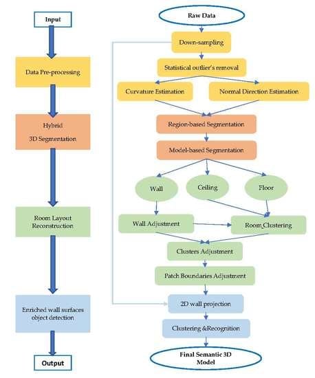
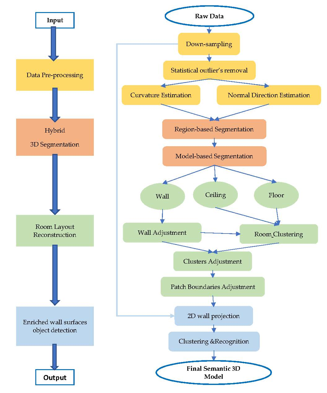
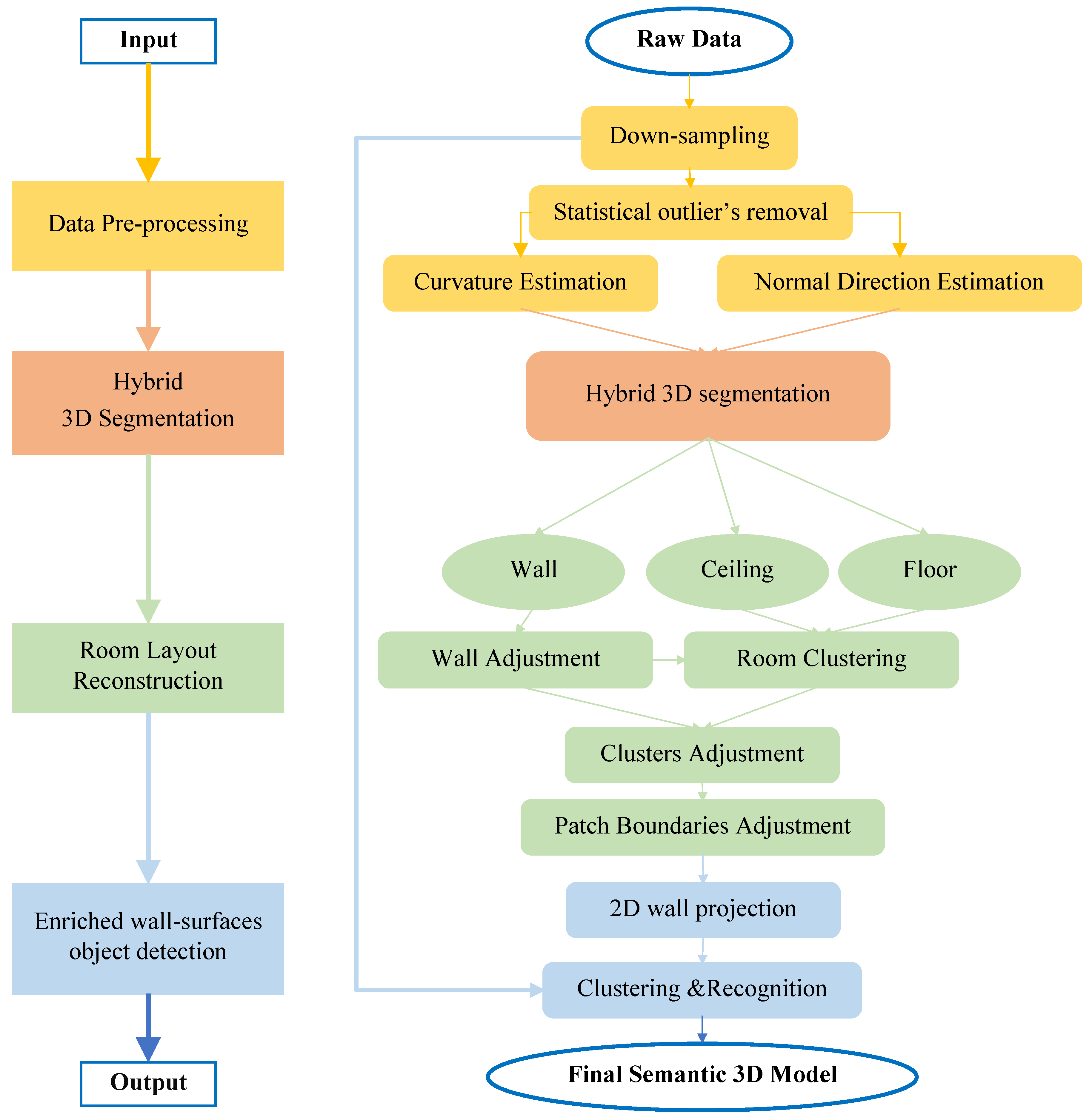
The proposed method automatically detects indoor building structural elements and wall-surface objects from an unstructured point cloud via four main steps, as shown in Figure 1. The method starts with a preprocessing step that prepares the raw point cloud by using down-sampling [5], outlier removal [20], and local surface properties calculation (i.e., normal, and surface variation (curvature)) using principal component analysis [4]. After local surface properties are estimated, the dataset is ready for the second step: 3D point cloud segmentation. A hybrid segmentation approach is thus introduced using region-based segmentation and model-based segmentation to estimate the planar surfaces. These planar surfaces are used for room layout reconstruction by re-orientating planar surfaces and segmented to main structural elements (i.e., wall, floor, ceiling), followed by clustering the ceiling for the detection of separate rooms. Room boundaries are detected for each room cluster using a modified convex hull algorithm [21] and line growing further development [3]. The clustered boundaries are adjusted using the detected wall planar segments. The newly estimated room cluster boundaries are used to detect wall-surface objects using a minimum graph cut algorithm [10]. Finally, all detected surfaces are modeled and exported with suitably formatted semantic information that can define each room cluster, structural elements for each room, as well as wall-surface objects. The details of each step are given and discussed in the following sub-sections.
3.2. Preprocessing
Using raw data for building modelling is not appropriate, as such data have an excess of unrequired information. The preprocessing of the raw data has a crucial impact on the required results, in that things, such as noise and outliers are removed. The raw point cloud dataset was subjected to two types of filter: Down-sampling and statistical outlier removal.
3.2.1. Down-Sampling
For an unstructured set of points p in 3D space ℝ3, all directions of the whole domain are divided into small cubes with the same grid space which is called a voxel. Each voxel containing points (1, 2, 3, …, n), is then replaced by one-point p. The desired characteristic —in our approach it is point spatial position—is calculated using the arithmetic average, as described by Equation (1). The down-sampling does not change the whole trend of the shapes but reduces the amount of data depending on the voxelization grid space used and the cloud density.
3.2.2. Statistical Outlier Removal
After the dataset is down-sampled, it may contain some outliers, such as sparse points collected from the scanner. Those points are detected based on their local distance to their neighbors [22]. To remove outliers from the dataset, statistical analysis takes place using location and scale parameters: Median and mean absolute deviation (MAD) instead of mean and standard deviation, because of its more robust ability to detect outliers [20].
3.2.3. Local Surface Properties
Local surface properties are required as inputs for segmentation and primitive’s detection. Two factors from local properties: Normal and surface variation (curvature) are estimated using the local neighborhoods of sample points. As demonstrated by References [7,23], the analysis of the covariance matrix is effective in estimating local properties. As the covariance matrix can be estimated by the nearest neighbors (k) as described in Equation (2), that computation can be conveyed to an eigenvectors problem as described in Equation (3). Considering the eigenvectors problem, the minimum eigenvector refers to the plane normal direction for that set of neighbors. Moreover, eigenvalues measure the variation in a set of neighbors together with the direction of eigenvectors, and curvature can be estimated using Equation (4).
where is the mean in the 3D of the neighborhood with size , and and are the respective eigenvectors and eigenvalues.
Note that the maximum curvature is equal to 1/3 which means that the points are isotropically distributed, and the minimum is equal to zero which means that all points are on the plane.
3.3. Hybrid 3D Point Segmentation
There are two different approaches for 3D point segmentation: Region-based and model-based approaches. In high-quality data with no furniture, each 3D segmentation approach can be implemented with acceptable results. Meanwhile, in low-quality data, such as a backpack laser system with full furniture, none of the 3D segmentation approaches can be effective. A new hybrid segmentation approach of combining a region-based approach [24] and a model-based approach [25] is implemented for the segmentation of planar surfaces.
Our hybrid segmentation goal is planar surfaces from the raw point cloud, so a seed point is selected with low curvature and the region is grown up based on predetermined difference angle threshold between region mean and the new points. The region is then segmented to different planar surfaces using RANSAC. In 3D space ℝ3, any point located in the plane surface can be represented by plane normal direction () and point coordinates (), as described in Equation (5). The perpendicular projected distance () from any point in space and the plane can be estimated using plane normal direction and the point coordinate as described in Equation (6).
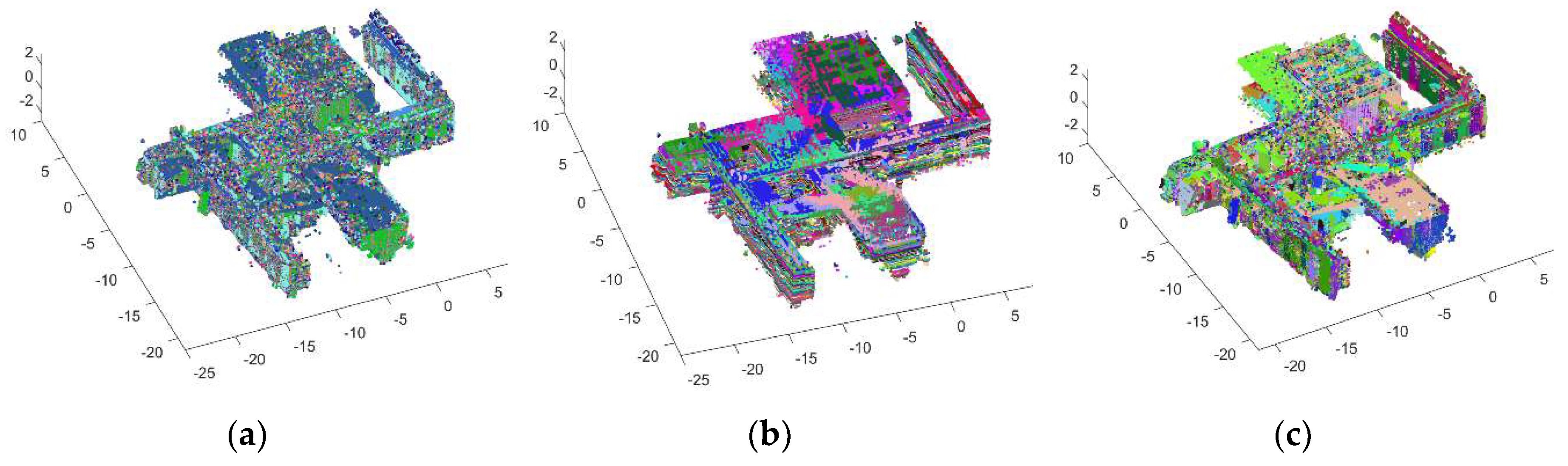
RANSAC is applied for the segmented point cloud, three random points are chosen to estimate plane model parameters, and all points are checked with the perpendicular projected distance. If that distance is within the threshold—wall thickness in our case—a new point is added to the plane points. Otherwise, the next point is selected. That procedure is reproduced several times, and a model with a high number of points is selected from all datasets. This step is repeated several times until the size of the region is less than the minimum predetermined threshold. As our interest is with planar surfaces, the procedures are continued with seed points until the curvature is greater than the threshold. Figure 2 shows the difference between using our hybrid approach, and another two approaches.
3.4. Room Layout Reconstruction
After the determination of all primitives, we are interested in the definition of each room patch, inclusive of its wall boundaries. This step consists of six main stages: Re-orientation and ceiling detection, wall refinement, room clustering, boundaries re-construction, in-hole reconstruction, and boundary line segments refinement.
3.4.1. Re-Orientation and Ceiling Detection
As different factors affect the data acquisition procedures and error propagation affects the orientation of the dataset, re-orientation of the detected primitives is estimated to ensure accurate positioning and modelling. Firstly, the primitives are classified as wall planes which are almost perpendicular to the vertical direction (gravity), and the other primitives are classified as ceiling or floor based on their average height. Three main dominant directions are estimated based on the plane of maximum points and the orthogonality of these planes. The generated local system (xyz) is compared to the gravitational Cartesian system (XYZ), and rotational angles (ω, φ, κ) are estimated. Then, the rotational matrix can be computed [26]. The results from that step are re-oriented and classified as planes: Wall, ceiling, and floor.
3.4.2. Wall Refinement
The vertical planes classified as wall structures need to be pruned. Because of the noise in the point cloud, some vertical planes may not belong to wall structures. These planes are pruned using region growing, histogram, and probability analysis. For each wall plane, region growing is applied to remove outliers. All points related to each vertical plane are projected to that plane and rasterized using a predefined pixel size. The 2D projected plane histogram is calculated, and the histogram is converted to a binary system (0 for zero pixels, and 1 if greater than zero). It is known that wall planes have distributed points over the whole plane, as shown in Figure 3d. Otherwise, it is considered to be a false plane (Figure 3c). Hence, a probability distribution function (PDF) is estimated for non-empty cells. If the PDF exceeds a predefined threshold, the plane is considered to be a wall structure.
3.4.3. Room Clustering
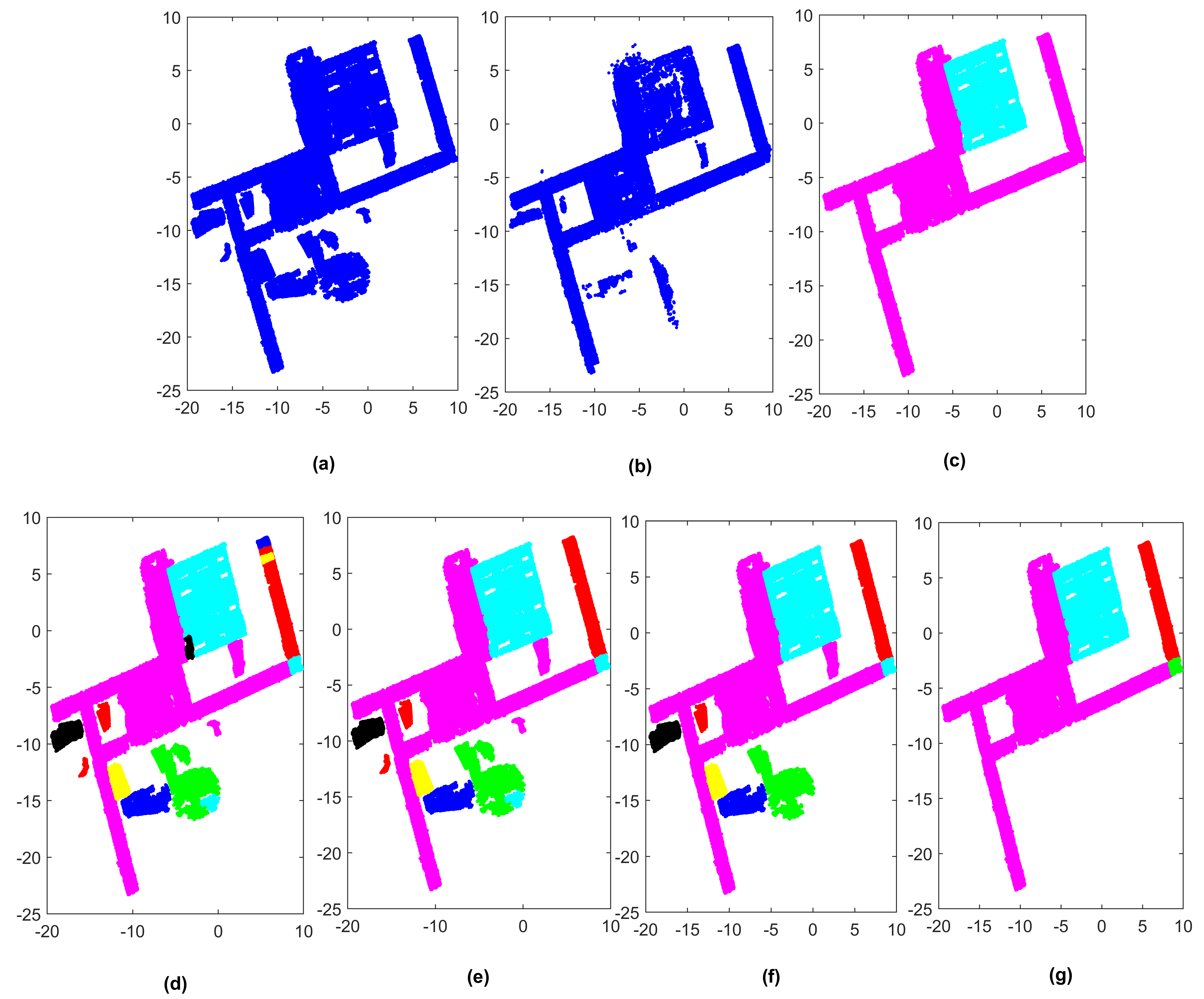
Clustering the whole floor to different room patches is our goal in that step, and the ceiling patch is the main feature used for clustering by using a region growing algorithm [27,28]. A seed point is randomly selected, and the region growing algorithm continually adds points to the same region if the Euclidean distance in 3D space is within a predefined threshold. The segmentation process might lead to over-segmentation (Figure 4d), thus wall segments and floor cluster are used to refine the clustering process.
Merging overlapped regions with no wall segments in the overlapped area (Figure 4d,e);
Merging overlapped regions with wall segments, but no wall points in the overlapped area (Figure 4g,c);
Discarding regions with an overlapped area with floor less than a predetermined percentage (Figure 4f,g); and
Discarding regions of a small area (Figure 4e,f).
3.4.4. Boundaries Reconstruction
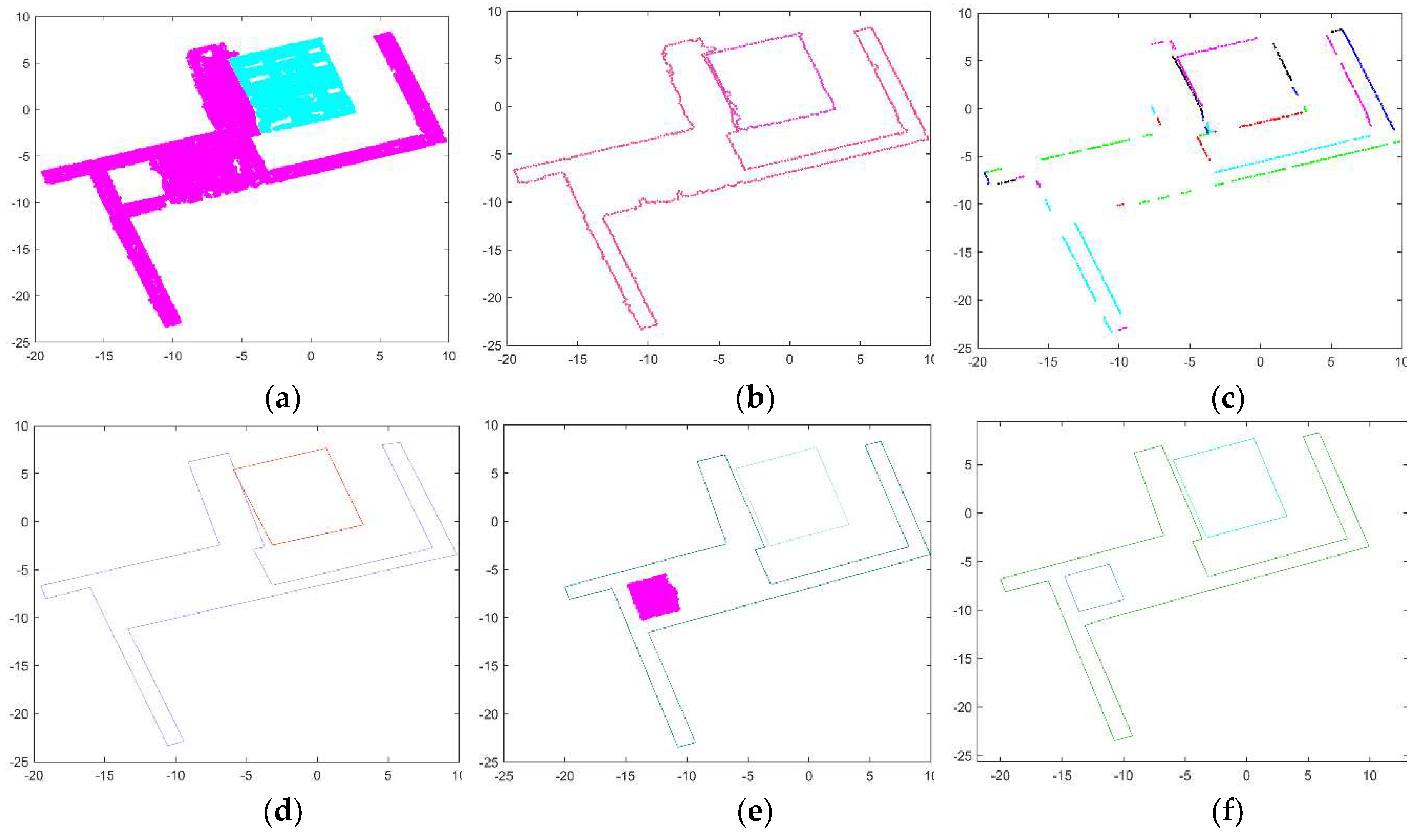
After the segmentation of room patches, we aim to reconstruct the boundaries of each room patch. These boundaries are estimated in 2D space. First, the boundaries for each region are traced by using a modified convex hull algorithm [21]. Circle neighborhood is adopted using a predefined radius, and the lower point in the {y} direction is the start seed point. By following counter-clockwise order, all boundary points are added (Figure 5b). Secondly, these traced points are filtered using a line growing algorithm [3] to detect collinear points with their corresponding lines using the least square method and a 2D line equation with projected perpendicular distance (ppd). From the line Equation (7), 2D line model parameters (A, B) can be estimated using the first two points, then the ppd from the next point to that line is estimated using Equation (8). If the ppd lies inside the threshold, the line will grow up. Otherwise, the new line will start. The detected line segments are intersected to determine the room layout shape (Figure 5c,d).
where x and y are point coordinates, and A and B are 2D line model parameters.
3.4.5. In-Hole Reconstruction
After the determination of all boundaries for cluster elements, the room cluster might occasionally contain a ventilation hole, or sometimes not all rooms are able to be scanned due to other conditions. As the outer boundaries for each room segment were detected in the previous step, this step is intended to detect inner boundaries by detecting holes in ceiling clusters. All ceiling points are projected in 2D space, and the same procedures for determining empty space as for the wall refinement step are conducted. Regions which lie inside outer boundaries of each room are kept, and boundary tracing and modelling procedures are implemented to detect hole points (Figure 5e,f).
3.4.6. Boundary Line Segments Refinement
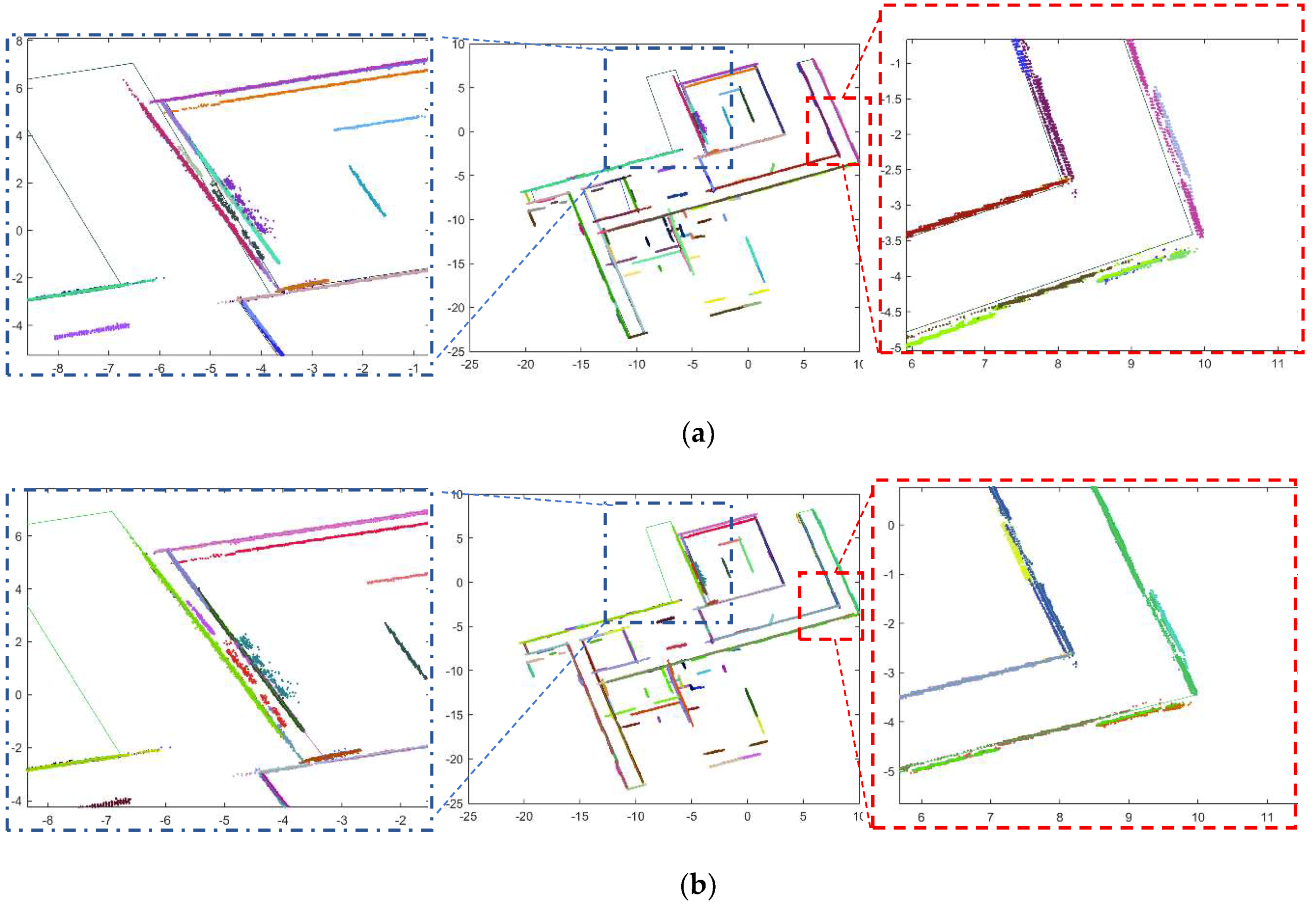
As points near boundaries have high curvature, they might be discarded from the segmentation procedures. High curvature leads to the false geometrical alignment of room boundaries, thus a refinement step for these boundary lines is required. In that step, wall planes are projected in 2D space (see Equations (7) and (8)). Line boundaries are adjusted by being moved near projected wall plane parameters. If there is no nearby wall, the parameters are used as the same boundary line, as shown in Figure 6. After the above refinement step, the height of each room is estimated from their inner points for the ceiling and floor clusters. Structural elements of the whole dataset can be extracted by the end of this step in 3D space.
3.5. Enriched Wall-Surface Objects Detection
The detection of openings in walls is a crucial task, as furniture may occlude some parts of the wall structure and thus be detected as an opening. Our approach depends on empty spaces to detect wall-surface objects taking into account the existence of furniture, and the work will be converted as graph cut optimization using multiple features to differentiate between wall-surface objects and occluded parts, then classify wall-surface objects as windows, doors (opened/closed), and virtual openings.
As shown in Figure 1 (i.e., the enriched wall-surface objects detection part), procedures for wall surface reconstruction consist of two main steps: 2D wall projection, and clustering and recognition. In the first step, the point cloud—within a threshold distance less than 0.5 m—is projected to the wall plane inside its boundaries using a 2D projection equation and a perpendicularly projected distance. As we are interested in defining surfaces, such as doors, windows, and virtual openings, the processing is simplified to a 2D space with wall coordinates (i.e., height and length). The projected data are then gridded in small pixel size with a predefined threshold and estimated histogram on the projected wall. From the histogram analysis, wall surfaces are defined using an occupancy analysis [9,10]. It is known that the openings will consist of a few points in the histogram, thus the openings can be defined by that criteria. The detected empty spaces represent not only wall surface objects, but also occluded parts of the wall. To deal with this problem, a region growing algorithm is implemented, using threshold distance, enabling those clustered regions to be pruned using statistical analysis. Region growing is applied using a predefined threshold to differentiate between different opening patches. Some of the detected openings may be due to occlusion by furniture, so statistical analysis of each cluster, using peak points on both wall directions, takes place to prune the detected objects.
Once the clusters are modified, the empty patches are ready for detailed recognition as one of the wall-surface objects. For each cluster, five dimensional features are defined: Max width, max height, lower height position, max height position, and point density distribution. The problem will be converted to graph cut optimization [9,10], but with an object-based, rather than a cell-based problem. The problem is to deal with several objects and assign a label to each one. The graph cut is used to convert the problem to a binary solution which assigns {1} to the object, providing it fulfils the required conditions, or {0} otherwise [9,10,19].
The clustered regions are represented on the graph by nodes or vertices (V), and these nodes are connected by a set of edges (E). The node has two additional terminals {source (s), and sink (t)} which are linked by n-link. That set {s & t} represents the foreground and background of the graph. The graph cut is used to label s like a wall (w) or object (o) by minimizing energy function, and the equation of the energy function [29] is shown in Equation (9).
where the energy function has both a data term and a smoothness term .
The data term is responsible for penalizing the object that has points, close within the threshold distance, and thus covers the whole object using a probability function, as shown in Equations (10) and (11). Maximum probability means highly distributed points over all of the objects:
Meanwhile, the smoothness term consists of a knowledge-based analysis of an object (node), and contains three sub terms, as described in Equations (12)–(15).
The sub terms appearing in a smoothness term are defined as follows:
- ❖
- Area term (): This term penalizes the total area of the node based on the following criteria:
- ❖
- Floor ceiling term (): This term penalizes nodes, the centroid of which is near to ceilings or floors, based on the following criteria:
- ❖
- Linearity term (): This term penalizes nodes if the ratio between length and width is larger than the threshold as shown below:where : Mean, : Standard deviation, : Thresholds, : Upper, lower, ceiling, and floor heights, respectively.
The solution of the energy function is obtained by assigning the minimum energy to the associated label (o), otherwise assigning (w). After removing non-surface objects, these objects are assigned as windows, doors, or virtual openings based on both the distances of the lower height to the floor and the maximum width of the door. A window has a marginal distance from the floor, and virtual openings have a large size compared to doors.
4. Experiments and Discussion
4.1. Datasets Description
To verify the ability of the adopted approach to achieve more semantic and acceptable results, two types of datasets were used: Synthetic and BLS datasets. The synthetic datasets are shown in Figure 7a–c and had complex room layout structures, and were designed by Reference [8] for evaluating the modelling of indoor scenes. The BLS datasets, as shown in Figure 7d–f, were collected in the Land Surveying and Geo-Informatics department “LSGI” in the Hong Kong Polytechnic University. These datasets were collected with full furniture and different layout complexities. The first dataset (BLS1) was collected as a part of the south tower corridor with the meeting room, as shown in Figure 7d. The second dataset (BLS2) was collected in a study room (ZS604) with an inner complex structure, shown in Figure 7e, the third dataset (BLS3) was collected in the smart city lab (Figure 7f). These datasets contain doors, each with a different image (closed/opened) of different sizes and with different window sizes.
4.2. Parameter Settings
As the proposed method contains both data-driven and model-driven approaches, some parameters were used for the detection and recognition of different objects. These parameters were classified into four categories as given in Table 2. In the pre-processing step, the raw data was down-sampled using a 0.05-m voxel size which satisfied the data quality without losing information. A 1-m standard deviation was used to remove outliers within 16 neighbor points, then the same number of neighbors was used to estimate local properties for each point. In the hybrid 3D segmentation, the difference of normal angle used to segment the point cloud was 15 degrees, with 500 being the minimum number of points per plane, then the region was segmented to planar surfaces using a maximum perpendicular distance of 10 centimeters. A 5° angle threshold was used in the room layout construction to estimate vertical walls, and a 0.25 m distance was used for clustering. A 0.25 m circle radius was used to detect and define outer boundaries for regions based on 100 as a minimum number of points per region. For the line growing algorithm, a minimum number of points per line of five was used to estimate the main lines of the outer boundaries. The last category for wall-surface objects detection, half-meter distance to the wall, was used to define the points as belonging to the wall, the minimum width of the object was considered as 0.25 m, and the minimum area of the surface object was 0.5 m. The minimum height of the door was determined as 1.75 m, and the maximum width of the door was determined as 1.70 m, to differentiate doors, windows, and virtual openings. The parameters of energy function were then used as indicated in Table 2.
4.3. Evaluation
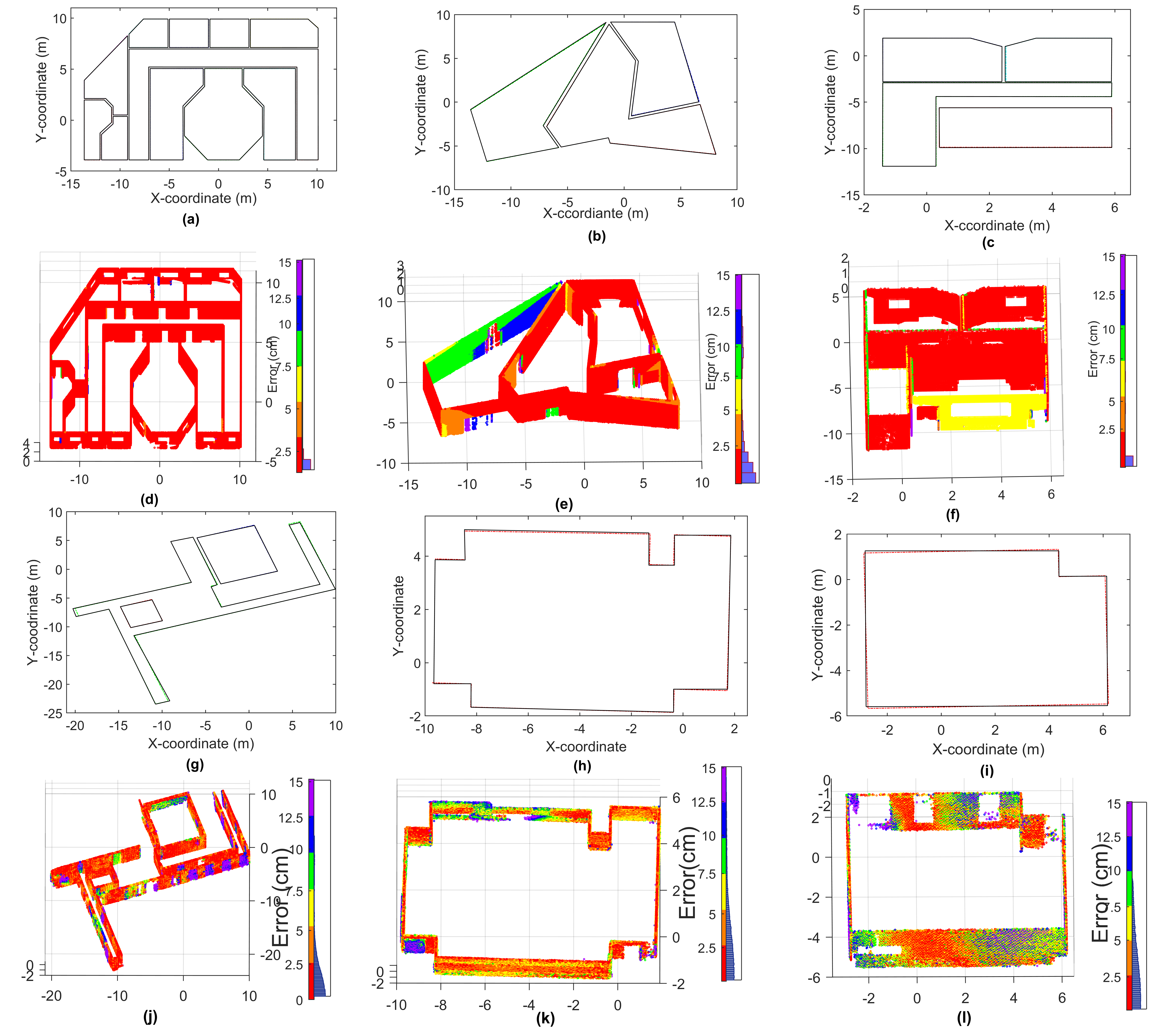
The proposed method was validated on both synthetic and BLS datasets. In a 2D domain, the reconstructed models were compared to the 2D floor plan generated from the datasets, as shown in Figure 8a–c for synthetic datasets, and as shown in Figure 8g–i for BLS datasets. Three different factors (i.e., precision, recall, and F-measure [30]) were used to evaluate the model, as described in Equations (16)–(18). Precession (P) defines the ratio between the intersection area—between the reconstructed model and the true shape—to the whole reconstructed area from the model, while recall (R) defines the ratio between the intersection area to the whole true area. In a 3D domain, point-to-plane distance errors are explained, as shown in Figure 8d–f for synthetic models and Figure 8j–l for BLS models.
The performance evaluation results in Table 3 show that our approach could reconstruct a model in 2D with a precession of around 99.2%, a recall of around 99.3%, and a harmonic factor of around 99.3%. Note that adjusting boundaries by using wall segments increased the accuracy of the reconstructed structural elements, which was obvious in high precession and recall results. The average error from point to plan in the 3D domain ranged from 0.5 to 2.0 cm for synthetic datasets and from 2 to 2.5 cm for BLS datasets.
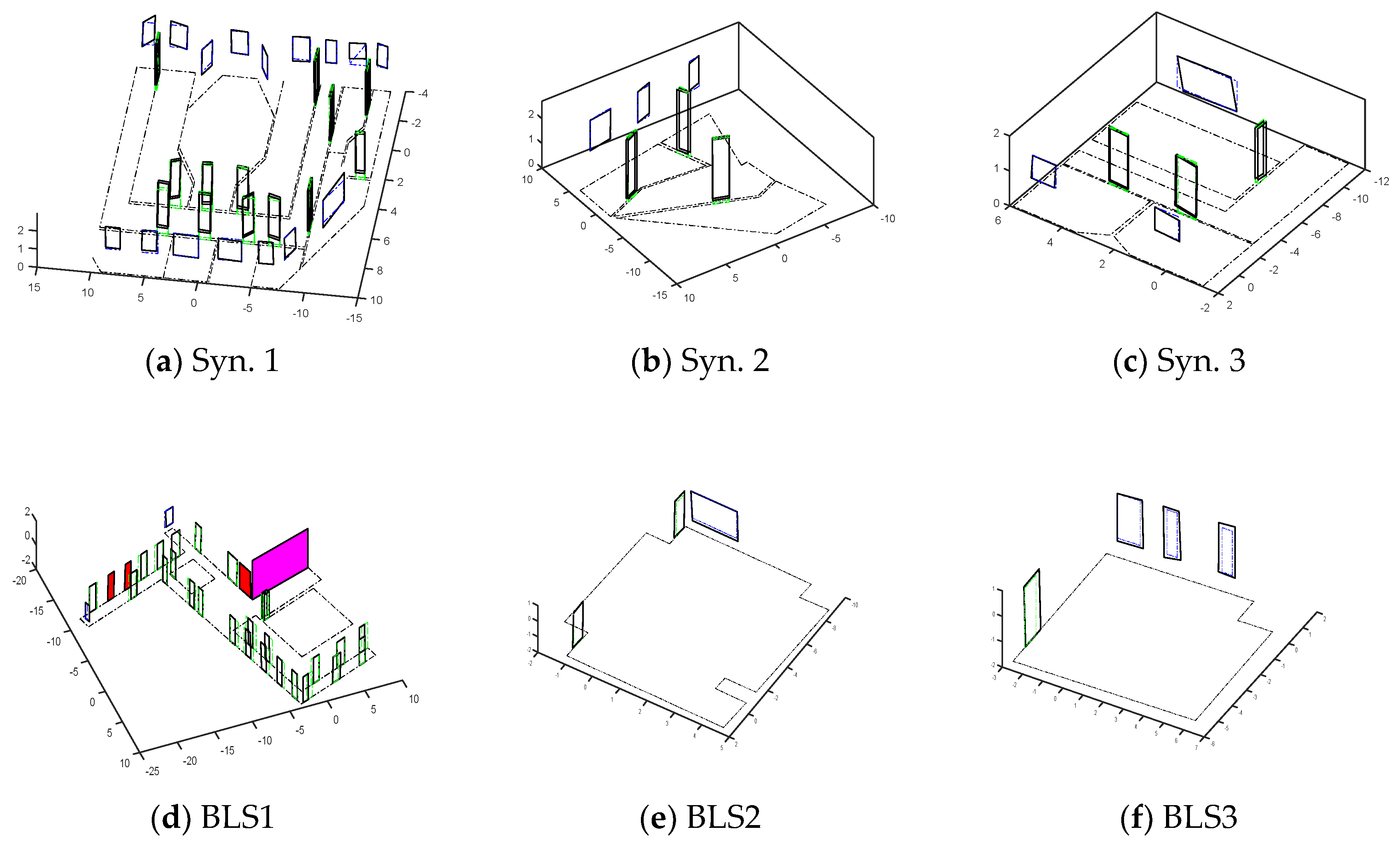
Besides, our approach could detect and model wall-surface objects, such as doors, windows, and virtual openings. Wall-surface objects were evaluated referring to quantity, as shown in Table 4, and quality as in Table 5, and were visualized, as shown in Figure 9. In Table 4, it is shown that all opened doors were detected, and most of the closed doors as well. Only in BLS3, three closed doors were not detected out of 23 doors, due to a small change in wall direction which affected the detection of these doors. One window out of four in BLS2 were detected, because of curtains which were pulled down which had an effect on the collected data. Virtual walls were detected with one more wall, due to the wall material of the two opposite walls affecting collecting points. For calculating precession and recall, reference models from raw datasets were compared with our approach results. From Table 5, a precession of around 90%, a recall of around 86%, and a harmonic factor of around 86.9% were obtained. The minimum precession for BLS1 of 76% was due to different door sizes and our assumption using same door width, and the minimum recall of 66% for BLS3 was for the same reason. From both 2D floor mapping and 3D wall surface objects, on synthetic datasets, our approach achieved a precision of around 94% and a recall of around 97%, while for BLS datasets our approach achieved a precision of around 95% and a recall of around 89%. For both datasets, the overall precession was around 95% with a recall of around 93%.
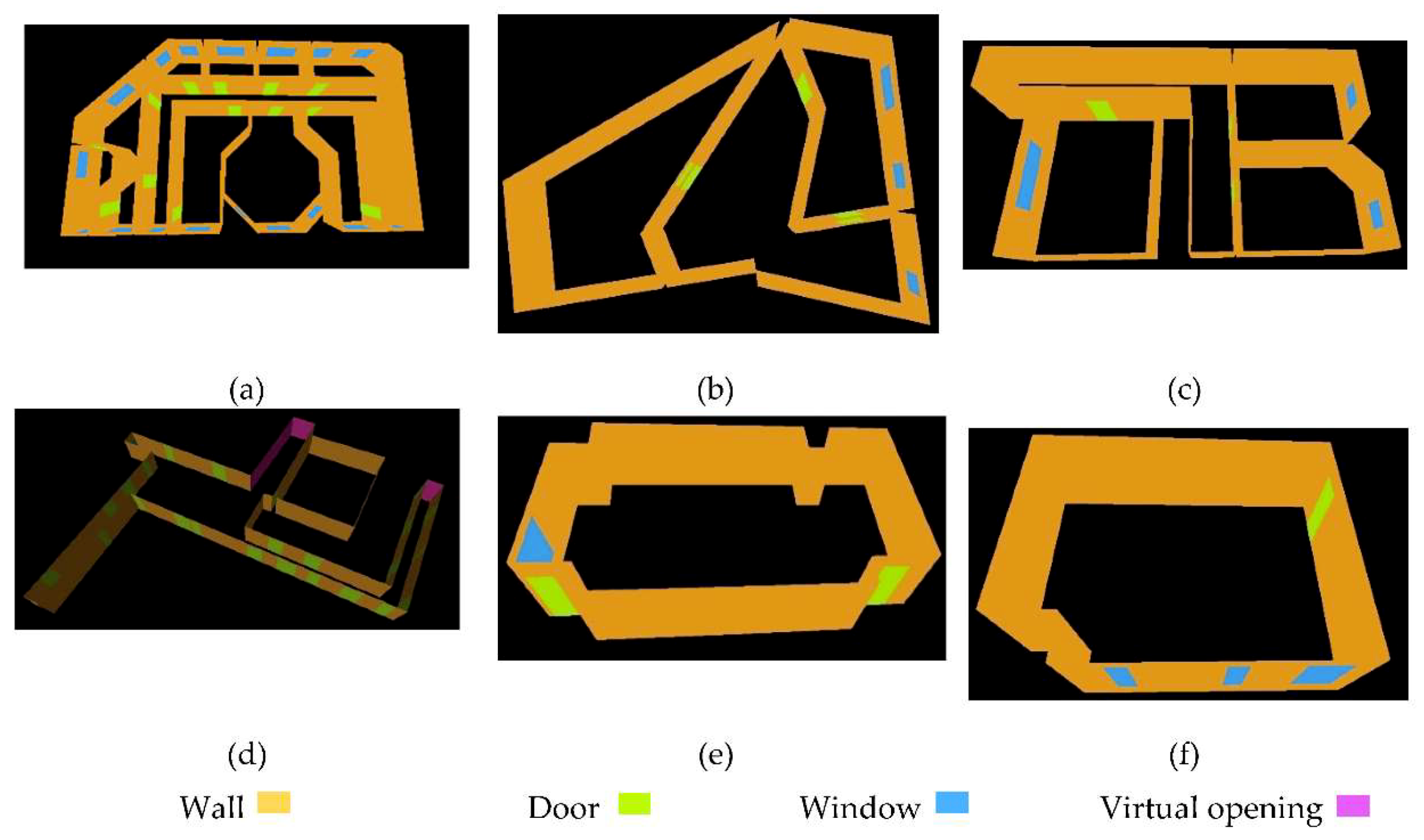
Final models are shown in Figure 10 for both synthetic datasets and BLS datasets. The final model is delivered with a semantic color for different classes of indoor scenes: Floor, ceiling, wall, door, window, and virtual opening, and the timing for each individual category referring to our implementation of the method is shown in Table 6. The code was written in MATLAB, and all tests were run on an Intel® Core™ i7-6700, 2.8 GHz processor.
5. Conclusions and Future Work
We presented our method to detect structural elements and wall-surface objects from BLS datasets. Our method could automatically construct a 2D floor plan of different room patches and a 3D model with semantic geometric information (i.e., ceiling, floor, door, window, and virtual opening). It showed the robustness of detection of separate room patches with complex layout structure, and their height could be estimated separately. At the level of wall-surface objects, it could detect opened doors, closed doors, and virtual openings. Compared to existing methods, our method does not require information about the line of sight or trajectory path. It uses a point cloud with geometric positions only, and it can also detect room patches with holes. In the future, we intend to enrich our approach for modelling irregularly shaped wall objects, detecting and modelling non-planar surfaces, recognizing in-room objects, and enrich our model with texture from synchronized images.
Author Contributions
Conceptualization, W.A.; Methodology, W.A.; Project administration, W.S.; Resources, N.L., W.F., H.X., and M.W.; Supervision, W.S.; Validation, W.A.; Writing—Original draft, W.A.; Writing—Review and editing, N.L.
Funding
This research is funded by RGC, grant number PF15-19401.
Acknowledgments
We would like to thank the anonymous reviewers for their insightful comments and substantial help on improving this article. This research is supported by projects: (a) Develop 3D Geodatabase Framework for Hong Kong – A Lightweight 3D Seamless Spatial Data Acquisition System (SSDAS) (ITP/053/16LP) and (b) A Preliminary Study on a High-order Markov Random Field-based Method for Semiautomatic Landslide Mapping Based on Remotely Sensed Imagery (G-YBN6. We acknowledge the Visualization and MultiMedia Lab at University of Zurich (UZH) and Claudio Mura for the acquisition of the 3D point clouds, and UZH, as well as ETH Zürich for their support with the synthetic datasets.
Conflicts of Interest
The authors declare no conflict of interest.
References
- Xiao, J.; Furukawa, Y. Reconstructing the World’s Museums. Int. J. Comput. Vis. 2014, 110, 243–258. [Google Scholar] [CrossRef] [Green Version]
- Cabral, R.; Furukawa, Y. Piecewise planar and compact floorplan reconstruction from images. In Proceedings of the 2014 IEEE Conference on Computer Vision and Pattern Recognition, Columbus, OH, USA, 23–28 June 2014; pp. 628–635. [Google Scholar]
- Dai, Y.; Gong, J.; Li, Y.; Feng, Q. Building segmentation and outline extraction from UAV image-derived point clouds by a line growing algorithm. Int. J. Digit. Earth 2017, 8947, 1–21. [Google Scholar] [CrossRef]
- Sanchez, V.; Zakhor, A. Planar 3D modeling of building interiors from point cloud data. In Proceedings of the 2012 19th IEEE International Conference on Image Processing, Orlando, FL, USA, 30 September–3 October 2012; pp. 1777–1780. [Google Scholar]
- Zhang, G.; Vela, P.A.; Brilakis, I. Detecting, Fitting, and Classifying Surface Primitives for Infrastructure Point Cloud Data. In Proceedings of the 2013 ASCE International Workshop on Computing in Civil Engineering, Los Angeles, CA, USA, 23–25 June 2013; pp. 6–9. [Google Scholar]
- Pang, Y.; Zhang, C.; Zhou, L.; Lin, B.; Lv, G. Extracting Indoor Space Information in Complex Building Environments. ISPRS Int. J. Geo-Inf. 2018, 7, 321. [Google Scholar] [CrossRef]
- Shaffer, E.; Garland, M. Efficient adaptive simplification of massive meshes. In Proceedings of the Conference on Visualization ’01, San Diego, CA, USA, 21–26 October 2001; pp. 127–551. [Google Scholar]
- Mura, C.; Mattausch, O.; Villanueva, A.J.; Gobbetti, E.; Pajarola, R. Automatic room detection and reconstruction in cluttered indoor environments with complex room layouts. Comput. Graph. 2014, 44, 20–32. [Google Scholar] [CrossRef] [Green Version]
- Wang, R.; Xie, L.; Chen, D. Modeling Indoor Spaces Using Decomposition and Reconstruction of Structural Elements. Photogramm. Eng. Remote Sens. 2017, 83, 827–841. [Google Scholar] [CrossRef]
- Michailidis, G.T.; Pajarola, R. Bayesian graph-cut optimization for wall surfaces reconstruction in indoor environments. Vis. Comput. 2017, 33, 1347–1355. [Google Scholar] [CrossRef]
- Lehtola, V.; Kaartinen, H.; Nüchter, A.; Kaijaluoto, R.; Kukko, A.; Litkey, P.; Honkavaara, E.; Rosnell, T.; Vaaja, M.T.; Virtanen, J.P.; et al. Comparison of the Selected State-Of-The-Art 3D Indoor Scanning and Point Cloud Generation Methods. Remote Sens. 2017, 9, 796. [Google Scholar] [CrossRef]
- Nguatem, W.; Drauschke, M.; Meyer, H. Finding Cuboid-Based Building Models in Point Clouds. ISPRS Int. Arch. Photogramm. Remote Sens. Spat. Inf. Sci. 2012, XXXIX-B3, 149–154. [Google Scholar] [CrossRef]
- Lin, Z.; Xu, Z.; Hu, D.; Hu, Q.; Li, W. Hybrid Spatial Data Model for Indoor Space: Combined Topology and Grid. ISPRS Int. J. Geo-Inf. 2017, 6, 343. [Google Scholar] [CrossRef]
- Ochmann, S.; Vock, R.; Wessel, R.; Klein, R. Automatic reconstruction of parametric building models from indoor point clouds. Comput. Graph. 2016, 54, 94–103. [Google Scholar] [CrossRef]
- Murali, S.; Speciale, P.; Oswald, M.R.; Pollefeys, M. Indoor Scan2BIM: Building Information Models of House Interiors. In Proceedings of the IEEE/RSJ International Conference on Intelligent Robots and Systems (IROS), Vancouver, BC, Canada, 24–28 September 2017. [Google Scholar]
- Ikehata, S.; Yan, H.; Furukawa, Y. Structured Indoor Modeling. In Proceedings of the ICCV, Las Condes, Chile, 11–18 December 2015. [Google Scholar]
- Coughlan, J.M.; Yuille, A.L. The Manhattan World Assumption: Regularities in Scene Statistics Which Enable Bayesian Inference. In Proceedings of the NIPS, Denver, CO, USA, 27 November–2 December 2000; pp. 845–851. [Google Scholar]
- Previtali, M.; Barazzetti, L.; Brumana, R.; Scaioni, M. Towards automatic indoor reconstruction of cluttered building rooms from point clouds. ISPRS Ann. Photogramm. Remote Sens. Spat. Inf. Sci. 2014, II-5, 281–288. [Google Scholar] [CrossRef]
- Oesau, S.; Lafarge, F.; Alliez, P. Indoor scene reconstruction using feature sensitive primitive extraction and graph-cut. ISPRS J. Photogramm. Remote Sens. 2014, 90, 68–82. [Google Scholar] [CrossRef] [Green Version]
- Leys, C.; Ley, C.; Klein, O.; Bernard, P.; Licata, L. Detecting outliers: Do not use standard deviation around the mean, use absolute deviation around the median. J. Exp. Soc. Psychol. 2013, 49, 764–766. [Google Scholar] [CrossRef] [Green Version]
- Sampath, A.; Shan, J. Building boundary tracing and regularization from airborne lidar point clouds. Photogramm. Eng. Remote Sens. 2007, 73, 805–812. [Google Scholar] [CrossRef]
- Knorr, E.M.; Ng, R.T. A Unified Notion of Outliers: Properties and Computation. In Proceedings of the International Conference on Knowledge Discovery and Data Mining, Newport Beach, CA, USA, 14–17 August 1997; pp. 219–222. [Google Scholar]
- Pauly, M.; Gross, M.; Kobbelt, L.P. Efficient simplification of point-sampled surfaces. In Proceedings of the 13th IEEE Visualization Conference, No. Section 4, Boston, MA, USA, 27 October–1 November 2002; pp. 163–170. [Google Scholar] [Green Version]
- Tovari, D.; Pfeifer, N. Segmentation based robust interpolation—A new approach to laser data filtering. Laserscanning 2005, 6. [Google Scholar]
- Schnabel, R.; Wahl, R.; Klein, R. Efficient RANSAC for Point-Cloud Shape Detection. Comput. Graph. Forum 2007, 26, 214–226. [Google Scholar] [CrossRef] [Green Version]
- Păun, C.D.; Oniga, V.E.; Dragomir, P.I. Three-Dimensional Transformation of Coordinate Systems using Nonlinear Analysis—Procrustes Algorithm. Int. J. Eng. Sci. Res. Technol. 2017, 6, 355–363. [Google Scholar]
- Maltezos, E.; Ioannidis, C. Automatic Extraction of Building Roof Planes from Airborne Lidar Data Applying an Extended 3d Randomized Hough Transform. ISPRS Ann. Photogramm. Remote Sens. Spat. Inf. Sci. 2016, III-3, 209–216. [Google Scholar] [CrossRef]
- Sampath, A.; Shan, J. Segmentation and reconstruction of polyhedral building roofs from aerial lidar point clouds. IEEE Trans. Geosci. Remote Sens. 2010, 48, 1554–1567. [Google Scholar] [CrossRef]
- Boykov, Y.; Veksler, O.; Zabih, R. Fast approximate energy minimization via graph cuts. IEEE Trans. Pattern Anal. Mach. Intell. 2001, 23, 1222–1239. [Google Scholar] [CrossRef] [Green Version]
- Chen, S.; Li, M.; Ren, K.; Qiao, C. Crowd Map: Accurate Reconstruction of Indoor Floor Plans from Crowdsourced Sensor-Rich Videos. In Proceedings of the International Conference on Distributed Computing Systems, Columbus, OH, USA, 29 June–2 July 2015; pp. 1–10. [Google Scholar]
Figure 1.
The overall process of the proposed method (different colors refer to different stages).

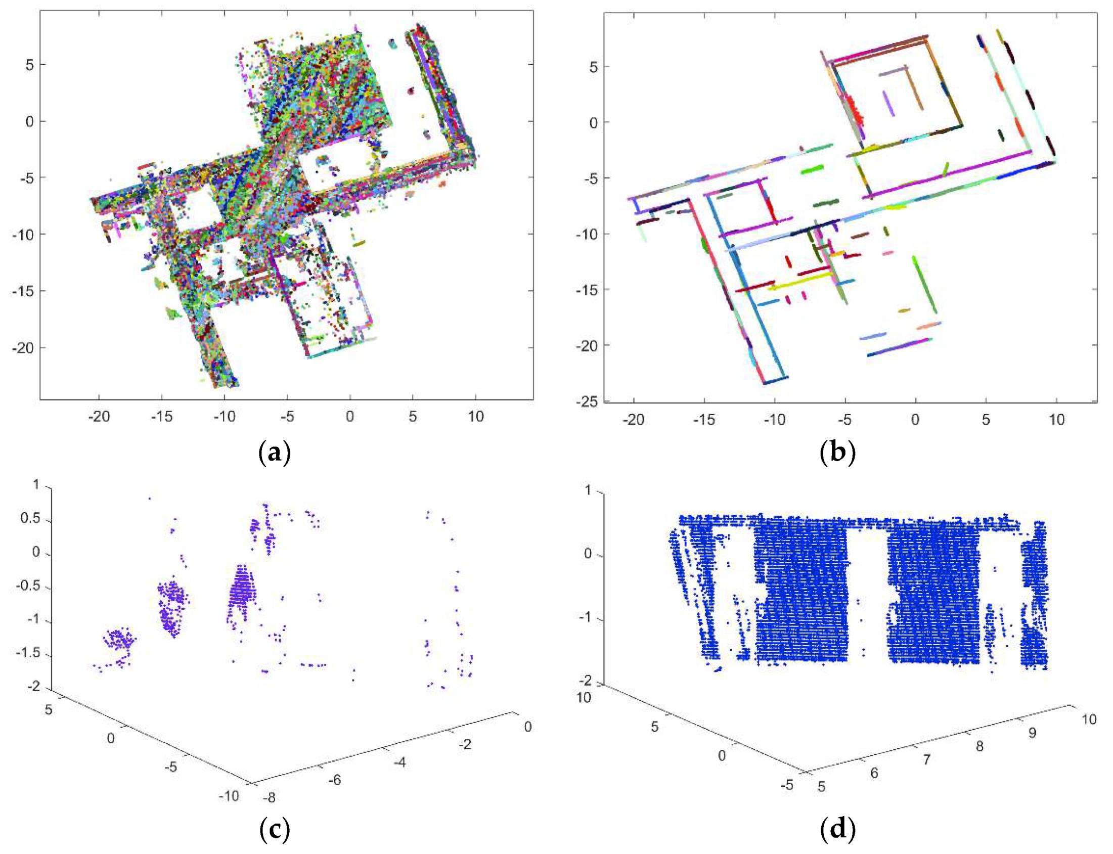
Figure 2.
3D point cloud segmentation: (a) Region-based; (b) model based; and (c) hybrid approach.

Figure 3.
Wall segments analysis: (a) Raw wall segments; (b) pruned wall segments; (c) side view of the false wall; and (d) side view of actual wall segments.
Figure 3.
Wall segments analysis: (a) Raw wall segments; (b) pruned wall segments; (c) side view of the false wall; and (d) side view of actual wall segments.

Figure 4.
Clustering procedures: (a,b) Ceiling and floor; (c) results; (d–g) enhancement of clusters.
Figure 4.
Clustering procedures: (a,b) Ceiling and floor; (c) results; (d–g) enhancement of clusters.

Figure 5.
Boundaries detection: (a) Room clusters, (b) detected boundary points, (c) detected line segments, (d) intersected lines, and (e,f) detecting holes and reconstructed segments.
Figure 5.
Boundaries detection: (a) Room clusters, (b) detected boundary points, (c) detected line segments, (d) intersected lines, and (e,f) detecting holes and reconstructed segments.

Figure 6.
Adjustment of wall segments using points of vertical planes: (a) Before adjustment; and (b) after adjustment.
Figure 6.
Adjustment of wall segments using points of vertical planes: (a) Before adjustment; and (b) after adjustment.

Figure 7.
The datasets used for evaluating our approach: (a–c) Synthetic datasets [8], and (d–f) backpack laser scanner (BLS) datasets (colors indicate different height).
Figure 7.
The datasets used for evaluating our approach: (a–c) Synthetic datasets [8], and (d–f) backpack laser scanner (BLS) datasets (colors indicate different height).

Figure 8.
(a–f) Evaluation of reconstructed models from synthetic datasets: (a–c) Comparison of the 2D floor plans (black lines) and reconstructed models (colored lines), and (d–f) distance of points to the nearest reconstructed plane (a histogram of errors is shown at right side). (g–l) Evaluation of reconstructed models from BLS: (g–i) Comparison of the 2D floor plans (black lines) and reconstructed models (colored lines), and (j–l) distance of points to the nearest reconstructed plane (a histogram of errors is shown at right side).

Figure 9.
Evaluation of wall-surface objects from the constructed model from our approach (blue color for the window, green color for the door) and reference model (black color) for (a–c) synthetic datasets and (d–f) BLS datasets. (red polygon for missed doors, and a magenta polygon for false virtual opening).

Figure 10.
Visualization of reconstructed models from (a–c) synthetic datasets and (d–f) BLS datasets (ceiling was removed for better visualization).
Figure 10.
Visualization of reconstructed models from (a–c) synthetic datasets and (d–f) BLS datasets (ceiling was removed for better visualization).


Table 1.
Comparison of existing approaches for indoor modelling. SE, structural element; Wo, window; Do, door; and VO, virtual opening; RGBD, red green blue depth.
Table 1.
Comparison of existing approaches for indoor modelling. SE, structural element; Wo, window; Do, door; and VO, virtual opening; RGBD, red green blue depth.
| Approach | Data Type | Main Concept | Final Model | ||||
|---|---|---|---|---|---|---|---|
| SE | Do | Wi | VO | Texture | |||
| [1] | Images Laser scanner | Manhattan world assumption Scanner position | ✓ | ✕ | ✕ | ✕ | ✓ |
| [2] | Panoramic images | Manhattan world assumption | ✓ | ✕ | ✕ | ✕ | ✓ |
| [16] | Panoramic RGBD images | Manhattan world assumption | ✓ | ✕ | ✕ | ✕ | ✓ |
| [15] | RGBD | Manhattan world assumption | ✓ | ✓ | ✕ | ✕ | ✕ |
| [14] | Terrestrial laser scanner | Scanner position | ✓ | ✓ | ✓ | ✓ | ✕ |
| [9] | Mobile laser scanner | Laser scanner trajectory | ✓ | ✓ | ✕ | ✕ | ✕ |
| [10] | Terrestrial laser scanner | Scanner position | ✕ | ✓ | ✓ | ✕ | ✕ |
Table 2.
Parameters used in the proposed approach. Ppd, projected perpendicular distance.
| Parameter | Value | Units | Parameter | Value | Units |
|---|---|---|---|---|---|
| Preprocessing | |||||
| Voxel size | 0.05 | meter | # of point neighbors | 16 | - |
| Outliers distance threshold | 1.0 | meter | |||
| Hybrid 3D Point Segmentation | Wall-Surface Reconstruction | ||||
| ppd | 0.1 | meter | Minimum width | 0.25 | meter |
| Area | 0.5 | square meter | Distance to wall | 0.5 | meter |
| Difference angle | 15 | degree | Door height | 1.75 | meter |
| # of points per plane | 500 | - | Door Width | 1.7 | meter |
| Room Layout Construction | Rasterization space | 0.1 | meter | ||
| # of points per region | 100 | - | Region distance | 0.2 | meter |
| R, region distance | 0.25 | meter | 0.5 | - | |
| ppd | 0.025 | meter | 0.5 | - | |
| # of points per line | 5 | meter | 0.6 | - | |
| Difference angle | 5 | degree | 3 | - | |
Table 3.
Evaluation of the reconstructed models compared to reference 2D floor plane.
| Precession (P) % | Recall (R) % | Harmonic Factor (F) % | |
|---|---|---|---|
| Syn. 1 | 99.8 | 99.8 | 99.8 |
| Syn. 2 | 99.7 | 99.2 | 99.5 |
| Syn. 3 | 99.7 | 99.5 | 99.6 |
| BLS1 | 97.4 | 99.1 | 98.2 |
| BLS 2 | 99.5 | 99.3 | 99.4 |
| BLS 3 | 99.3 | 99 | 99.2 |
Table 4.
Statistics of the output models compared to input datasets for wall-surface objects. Wo, window; Do, door; VO, virtual Opening. {out/input}.
Table 4.
Statistics of the output models compared to input datasets for wall-surface objects. Wo, window; Do, door; VO, virtual Opening. {out/input}.
| Down-Sampled % | Do (Opened) | Do (Closed) | Wi | VO | |
|---|---|---|---|---|---|
| Syn. 1 | 1 | 13/13 | - | 16/16 | - |
| Syn. 2 | 2 | 3/3 | - | 3/3 | - |
| Syn. 3 | 1 | 4/4 | - | 3/3 | - |
| BLS 1 | 1.5 | 5/5 | 23/20 | 100 | 2/3 |
| BLS 2 | 0.1 | 1/1 | 1/1 | 4/1 | - |
| BLS 3 | 0.6 | 1/1 | - | 3/3 | - |
Table 5.
Evaluation of wall-surface objects in different datasets.
| Precession (P) % | Recall (R) % | Harmonic Factor (F) % | |
|---|---|---|---|
| Syn. 1 | 84.7 | 90.1 | 86.1 |
| Syn. 2 | 91.7 | 98.7 | 95.0 |
| Syn. 3 | 91.7 | 95.4 | 93.5 |
| BLS 1 | 76.0 | 87.6 | 79.7 |
| BLS 2 | 97.6 | 81.4 | 88.50 |
| BLS 3 | 99.1 | 65.9 | 78.7 |
Table 6.
Time cost (in seconds) for our proposed approach on the tested datasets.
| Dataset | Preprocessing | Hybrid Segmentation | Room Layout Reconstruction | Enriched Wall-Surface Object Detection |
|---|---|---|---|---|
| Syn. 1 | 95.91 | 49.78 | 468.14 | 69.30 |
| Syn. 2 | 33.38 | 23.20 | 281.29 | 39.68 |
| Syn. 3 | 37.16 | 6.90 | 278.32 | 37.313 |
| BLS 1 | 161.53 | 219.16 | 164.18 | 39.91 |
| BLS 2 | 31.25 | 48.03 | 105.24 | 28.35 |
| BLS 3 | 60.72 | 24.71 | 112.45 | 29.45 |
© 2018 by the authors. Licensee MDPI, Basel, Switzerland. This article is an open access article distributed under the terms and conditions of the Creative Commons Attribution (CC BY) license (http://creativecommons.org/licenses/by/4.0/).
Share and Cite
MDPI and ACS Style
Shi, W.; Ahmed, W.; Li, N.; Fan, W.; Xiang, H.; Wang, M. Semantic Geometric Modelling of Unstructured Indoor Point Cloud. ISPRS Int. J. Geo-Inf. 2019, 8, 9. https://0-doi-org.brum.beds.ac.uk/10.3390/ijgi8010009
AMA Style
Shi W, Ahmed W, Li N, Fan W, Xiang H, Wang M. Semantic Geometric Modelling of Unstructured Indoor Point Cloud. ISPRS International Journal of Geo-Information. 2019; 8(1):9. https://0-doi-org.brum.beds.ac.uk/10.3390/ijgi8010009
Chicago/Turabian StyleShi, Wenzhong, Wael Ahmed, Na Li, Wenzheng Fan, Haodong Xiang, and Muyang Wang. 2019. "Semantic Geometric Modelling of Unstructured Indoor Point Cloud" ISPRS International Journal of Geo-Information 8, no. 1: 9. https://0-doi-org.brum.beds.ac.uk/10.3390/ijgi8010009
Note that from the first issue of 2016, this journal uses article numbers instead of page numbers. See further details here.