Spatiotemporal Influence of Urban Environment on Taxi Ridership Using Geographically and Temporally Weighted Regression

Abstract

Taxicabs play an important role in urban transit systems, and their ridership is significantly influenced by the urban built environment. The intricate relationship between taxi ridership and the urban environment has been explored using either conventional ordinary least squares (OLS) regression or geographically weighted regression (GWR). However, time constitutes a significant dimension, particularly when analyzing spatiotemporal hourly taxi ridership, which is not effectively incorporated into conventional models. In this study, the geographically and temporally weighted regression (GTWR) model was applied to model the spatiotemporal heterogeneity of hourly taxi ridership, and visualize the spatial and temporal coefficient variations. To test the performance of the GTWR model, an empirical study was implemented for Xiamen city in China using a set of weekday taxi pickup point data. Using point-of-interest (POI) data, hourly taxi ridership was analyzed by incorporating it to various spatially urban environment variables based on a 500 × 500 m grid unit. Compared to the OLS and GWR, the GTWR model obtained the best performance, both in terms of model fit and explanatory accuracy. Moreover, the urban environment was revealed to have a significant impact on taxi ridership. Road density was found to decrease the number of taxi trips in particular places, and the density of bus stops competed with taxi ridership over time. The GTWR modelling provides valuable insights for investigating taxi ridership variation as a function of spatiotemporal urban environment variables, thereby facilitating an optimal allocation of taxi resources and transportation planning.

1. Introduction

Taxicabs are an indispensable component of modern metropolis transportation, by supplementing other public transport modes in terms of a flexible floating services and all-day operation. The significance of the taxi industry is usually measured by its fleet size and number of passengers. According to the government’s report for Beijing, by the end of 2014, there were 67,546 urban taxicabs in Beijing carrying approximately 1.88 million passengers daily. However, with recent acceleration in the carpooling mode, a significant obstacle for the taxi industry involves effectively augmenting transportation planning and improving the quality of their services, and ultimately realizing the aim of promoting urban transport systems [1]. To this end, it is critical that causative factors influencing taxi ridership are identified, and that the spatiotemporal development of these influencing factors is evaluated [2]. Elucidating the elements that determine taxi ridership will allow transit authorities to effectively apportion limited resources for transit service deployment, as well as prepare further pointed procedures for pricing and investment [3].

However, exploring urban taxi ridership remains a comprehensive task. Research into factors influencing transit ridership over the last few decades can be reduced to two categories [4]. The first category includes descriptive analyses based on survey and interview data, including fare development, marketing strategies, and other approaches or policies originating from the departments governing transit systems. The data on internal factors is likely to be biased due to circumscribed or incorrect information. This inherent data deficiency thus limits the applicability of descriptive research on transit ridership. The second category utilizes causal analyses to evaluate significant aspects of transit ridership. These models have been applied in complex empirical analyses to elucidate ridership, using of internal and external variables [5]. In contrast to descriptive analyses, causal analyses typically incorporate data that are less subjective and obtained from multiple sources. Some earlier studies have implied that external factors have a larger influence on ridership than internal factors [6]. As an example, the urban environment—a crucial external factor constituent—actively influences commuter behaviors, thus causing an oscillation in taxi ridership [7]. Previously published articles have recognized the substantial impact that land use attributes to the attractiveness of public transport [3], such as density, land use [8], and other appropriate determinants. Nonetheless, data aggregation and the collinearity of the variables in these models, result in contradictory and possibly spurious conclusions regarding the effects of important variables [9].

The traditional approaches to ridership analysis are dominated by ordinary least square (OLS) multiple regression models. The OLS model is cost-effective and suitable for multi-scale analysis [7,10]. In fact, as a global regression method, a prerequisite assumption of the OLS model is that all variables are stationary and independent across the study area. Since urban taxi trips are taken for multifarious purposes, and urban functionality varies over space and time, it is difficult to clearly articulate the determinants relevant to taxi ridership. Failing to capture the local variations will undoubtedly reduce the model’s reliability, and restrict the understanding of the spatial variation of taxi ridership [11]. Geographically weighted regression (GWR), as one of the alternatives to overcoming this drawback [12], allows independent variables to alter spatially, and explains unsteady effects. Meanwhile, it enables visualization of regression coefficients’ local variation. It is, therefore, widely used to interpret the spatial heterogeneity of geographical data [13].

Similar to spatial non-stationarity, temporal non-stationarity represents the time-sensitive nature of taxi ridership, and will be affected by before or after situation. Therefore, when conducting ridership analysis, it is necessary to explicitly consider the spatial and temporal variations. However, modelling spatiotemporal data (e.g., ridership, air quality, and house price) using GWR requires dependent variables to be aggregated or averaged by means of a particular timestamp [14,15]. Temporal non-stationarity is usually omitted during the aggregating process [16].

Space and time are two fundamental dimensions relating to all geographic processes. The development of the geographic information system (GIS) and automatic global position system (GPS) collection technologies has rendered spatiotemporal analysis and geographic parameter modelling as the primary focuses of the geographical information science [17]. Examples include investigating the spatiotemporal patterns of real estate prices [18,19,20], environmental issues [21,22,23], etc. Despite the efficacious integration of the temporal dimension into spatial analysis and modelling in a variety of studies, the determinants of ridership by combining temporal non-stationarity with spatial characteristics, have only slightly been assessed when evaluating the association between transit ridership and the built environment [5].

In an attempt to address this, the present study assessed the spatiotemporal properties of the association between the urban environment and taxi ridership by means of a geographically and temporally weighted regression (GTWR) model [18]. After adding temporal non-stationarity, the GTWR model extended the conventional GWR model to integrate both temporal and spatial information into the analysis. In particular, time is treated as the third dimension in addition to location and distance in a straightforward manner, to calculate the spatial-temporal weight. Thus, this space–time regression model can simultaneously incorporate temporal information from the estimation time or from previous times into the spatial variability. Nevertheless, the predictive ability of GTWR at elucidating the relationship between taxi ridership and urban environment, especially based on per hour, has yet to be explored. Optimization of parameter values for GTWR is also required to reduce the computational cost for handling a big dataset.

In order to confirm the efficacy of the GTWR model in determining the association between transit ridership and the urban environment, an empirical study in Xiamen Island was applied. We validated the effectiveness of the GTWR model in identifying the spatiotemporal influence of the urban environment on taxi ridership using one weekday origin-destination (OD) data, and various POI information. Firstly, the taxi OD data with high fitting precision were pre-processed, and the spatial distribution of hourly taxi ridership was obtained per traffic analysis zone (TAZ). Second, the GTWR model was applied to evaluate the coefficients’ spatiotemporal pattern. The experimental results revealed that GTWR achieved significantly better fit than traditional OLS and GWR models. Moreover, the spatial and temporal variations of the coefficients were visualized based on the GTWR model. The fluctuation in coefficients over time was captured while the temporal dimension was added to the GTWR model.

The rest of this paper is arranged as follows. In Section 2, the developed framework of GTWR and its application for taxi ridership approximation is briefly summarized. Section 3 introduces the pre-processing process for a dataset of taxi ridership and POI in the city of Xiamen, China. The OLS, GWR, and GTWR model results are evaluated in Section 4. The estimation coefficients of the GTWR model are then spatially and temporally analyzed in Section 5. Section 6 ultimately considers the benefits of the GTWR model, and summarizes prospective research applications.

2. Methods

2.1. Geographically Weighted Regression Model

Multifactorial dynamic relationships are common in complex traffic systems where some predictors cannot be observed or addressed easily. Regression analysis is widely used to study the correlation between dependent and independent variables, e.g., linear regression, logistic regression, and log linear regression [24]. The OLS regression is the most representative model among statistical methods for revealing the complicated relationship between urban environment and transit ridership. The basic assumption of the OLS model is that ridership data are independent and stationary in space. However, taxi ridership from a TAZ do not normally conform to the hypothesis, because of the nonstationary spatial autocorrelation among its neighboring zones. Thus, the applicability of the OLS model to spatial modelling has been criticized for neglecting spatial variation.

The GWR model is a spatially varying coefficient regression model, which can significantly improve estimation accuracy, especially in a study area with a complex spatial distribution [12]. It can be described as an extension of multiple linear regression models by combining independent variables with geographical locations. Assuming the taxi ridership sample is designated Y_i, where i (i = 1, 2,…, n) represents a TAZ, the general form of GWR model for the independent (Y_i) and dependent variables (urban environment factors, X_ik) can be mathematically expressed as:

$$Y_i={\beta }_0(u_i,v_i)+{\displaystyle \sum _k{\beta }_k(u_i,v_i)X_{ik}}+{\epsilon }_i,$$

(1)

where (u_i, v_i) represents the given coordinates of the TAZ i in space location (u_i, v_i); β₀ is the intercept value; β_k denotes the slope for each urban environment factors X_ik; and ε_i is the random error. The variables X_ik are sensitivity factors to improve the association between taxi ridership and urban environment concentrations, such as road length/density, number/density of residential building, places of employment, and public services. Unlike the ‘fixed’ coefficient estimates over space in the OLS model, this model allows the parameter estimates to vary across space and therefore capture local effects.

However, this model ignores the fact that spatial variation could vary with time and may be dependent on previous days, which is also an important influential factor of taxi ridership. Thus, the GWR model is limited, because it cannot make use of temporal autocorrelation existing in spatiotemporal data.

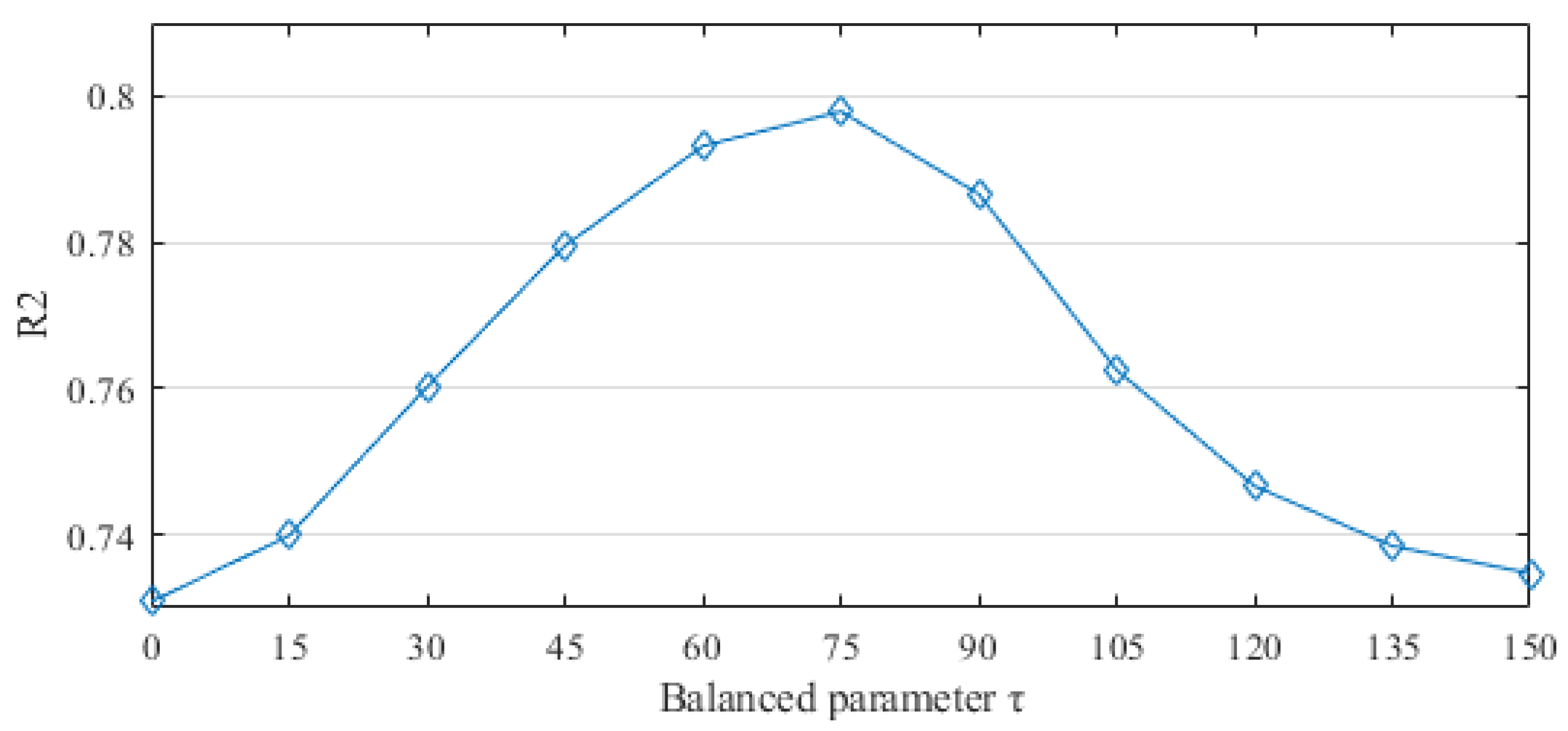
2.2. Geographically and Temporally Weighted Regression Model

Through integrating temporal effects into the GWR model, we proposed a GTWR model to simultaneously deal with the spatial and temporal non-stationarity issues [18]. In this article, the GTWR model was applied to improve the local coefficient of determination parameter for taxi ridership and the estimation of the urban environmental factors on an hourly basis. The general structure of the GTWR model that developed to estimate the spatiotemporal relationship between taxi ridership and point-of-interest (POI) data is described in detail in Equation (2).

$$Y_i={\beta }_0(u_i,v_i,t_i)+{\displaystyle \sum _k{\beta }_k(u_i,v_i,t_i)X_{ik}}+{\epsilon }_i,$$

(2)

where (u_i, v_i, t_i) represents the given coordinates of the TAZ i in space location (u_i, v_i) at time t_i; β₀, β_k, ε_i, and X_ik are the same as for the GWR model. To estimate the intercept of β₀ and the slopes of β_k for each variable, a locally weighted least squares method is usually employed. This assumes that the closer the measurements are to point i in the space-time coordinate system, the greater the weight of the measurements in predicting β_k. Thus, the estimation of coefficients is expressed as:

$$\widehat{\beta }(u_i,v_i,t_i)={[X^{T}W(u_i,v_i,t_i)X]}^{-1}{X}^{T}W(u_i,v_i,t_i)Y,$$

(3)

where X is a vector representing urban environmental factors. The space–time weight matrix W(u_i, v_i, t_i) was introduced to measure the importance of sample i to the estimated sample j, with respect to space and time. Considering the different scale effects of space and time, a simple ellipsoidal coordinate system has been introduced to measure the spatiotemporal distance between a regressive grid cell and its surrounding cells [18]. Through combining the temporal distance d^T with the spatial distance d^S, the spatiotemporal distance can be expressed as:

$$d^{ST}=d^s\otimes d^T,$$

(4)

where ‘⊗’ can represent different kinds of operators. In this context, we simplify selected ‘+’ as the combination operator to calculate the total spatiotemporal distance. The spatiotemporal distance between taxi ridership can thus be expressed as a linear weighting combination as indicated below:

$${(d_{ij}^{ST})}^2=\lambda [{(u_i-u_j)}^2+{(v_i-v_j)}^2]+\mu {(t_i-t_j)}^2,$$

(5)

where t_i and t_j constitute the observed time of ridership i and j. λ and μ are the weights for harmonizing the influences of differing units between space, distance, and time. If the common Gaussian distance decay-based functions and Euclidean distance are used to build the weight matrix, the weight matrix can be computed as indicated below:

$$\begin{array}{l}{W}_{ij}=\exp [-\frac{{(d_{ij}^{ST})}^2}{h_{ST}^{}{}^2}]\\ =\exp \{-\frac{[{(u_i-u_j)}^2+{(v_i-v_j)}^2]+\tau {(t_i-t_j)}^2}{h_s{}^2}\}\end{array}$$

(6)

where the parameter τ is a simplified ratio calculated by μ/λ (λ ≠ 0). In fact, the essential effect of τ is to balance the different scale between space distance and time distance. It should be noted that the scale factor τ is necessary. Otherwise, if d^S is much larger than d^T, d^ST will be dominated by d^S. This may degrade the temporal effect, and vice versa. To determine a reasonable τ, we can set λ = 1 to reduce the number of parameters in practice, and so that only μ has to be evaluated. μ can be optimized using cross-validation (CV) in terms of R², or Akaike information criterion (AIC) if a priori knowledge is unavailable.

h_ST is a positive parameter named the space–time bandwidth. This parameter can also be acquired either by means of a CV process via minimization in terms of R² statistics, or via the use of the AIC or the correct AIC [25] as follows:

$$CV(h)={\displaystyle \sum _i{[y_i-y_{\ne 1}(h_s)]}^2},$$

(7)

$$AIC=2k+nln\left(RSS\right),$$

(8)

where y_≠1(h_s) indicates the predicted value y_i from the GTWR model with a bandwidth h. Plotting CV(h) against the parameter h facilitates the selection of the optimum h. In Equation (8), k is the number of estimated parameters in the model, and n denotes sample size. Note that AIC with a correction (AICc) converges to AIC with the increase of n.

Figure 1 presents a flowchart of the proposed estimation method. Taxi ridership data acquired from the government, such as the pick-up and drop-off locations, was initially used to produce spatial distribution images with a base resolution of 500 m on a grid-based layer. Then, the statistics for the variables were extracted from the POI data and geo-registered, and then interpolated to the same coordinate system using the spatial analyst technology. Finally, hourly taxi ridership prediction maps at a 500 m resolution were produced using the three models, including OLS, GWR, and GTWR. In addition, a 10-fold CV technique was synchronously applied in three models, and the statistic of R², adjust R², AIC, RSS (residual sum of squares), RE (relative error), and RMSE (root mean square error) were calculated to assess the performance of model fitting and validation.

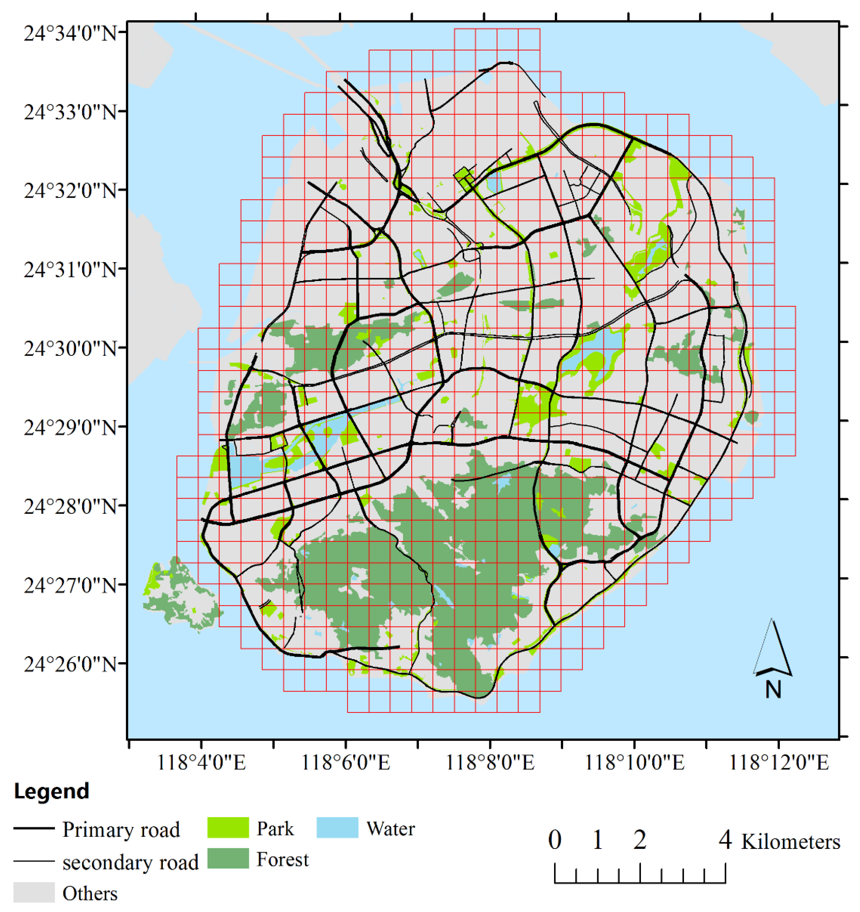
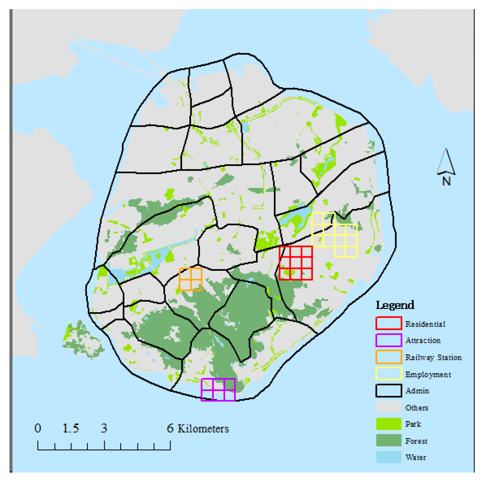
3. Study Area and Data

Xiamen City is located on the southeast coast of China (24°23′–24°54′ N latitude, 117°53′–118°26′ E longitude). It has a land area of more than 1700 km², and a sea area of 300 km². At the end of 2017, the city’s registered household population was four million. There are six administrative divisions, two on the island and four outside. Although Xiamen Island occupies only 10 percent of the total area of the city, nearly half of the population lives on the island, resulting in 92% of the taxi records being generated there. Therefore, Xiamen Island was selected for the case study (Figure 2). In an attempt to evaluate the impact of the urban environment on taxi ridership, we used an integrated dataset that includes land use and taxi pick-up locations. The grid cell was used as the geographical representative of the study area. We choose a grid cell instead of the administrative region for two reasons. The first is that the grid cell was more adaptable to multi-scale conditions, which can provide a reasonable scale to understand the spatial pattern of urban taxi ridership. The second is that its computational efficiency was higher, and it can easily handle large volumes of spatial data. After several tests, we used 500 m as the appropriate resolution for grid cell size. The final shape file of the study area contained 693 grid cells, with all pickup locations being subsequently aggregated into the corresponding cells.

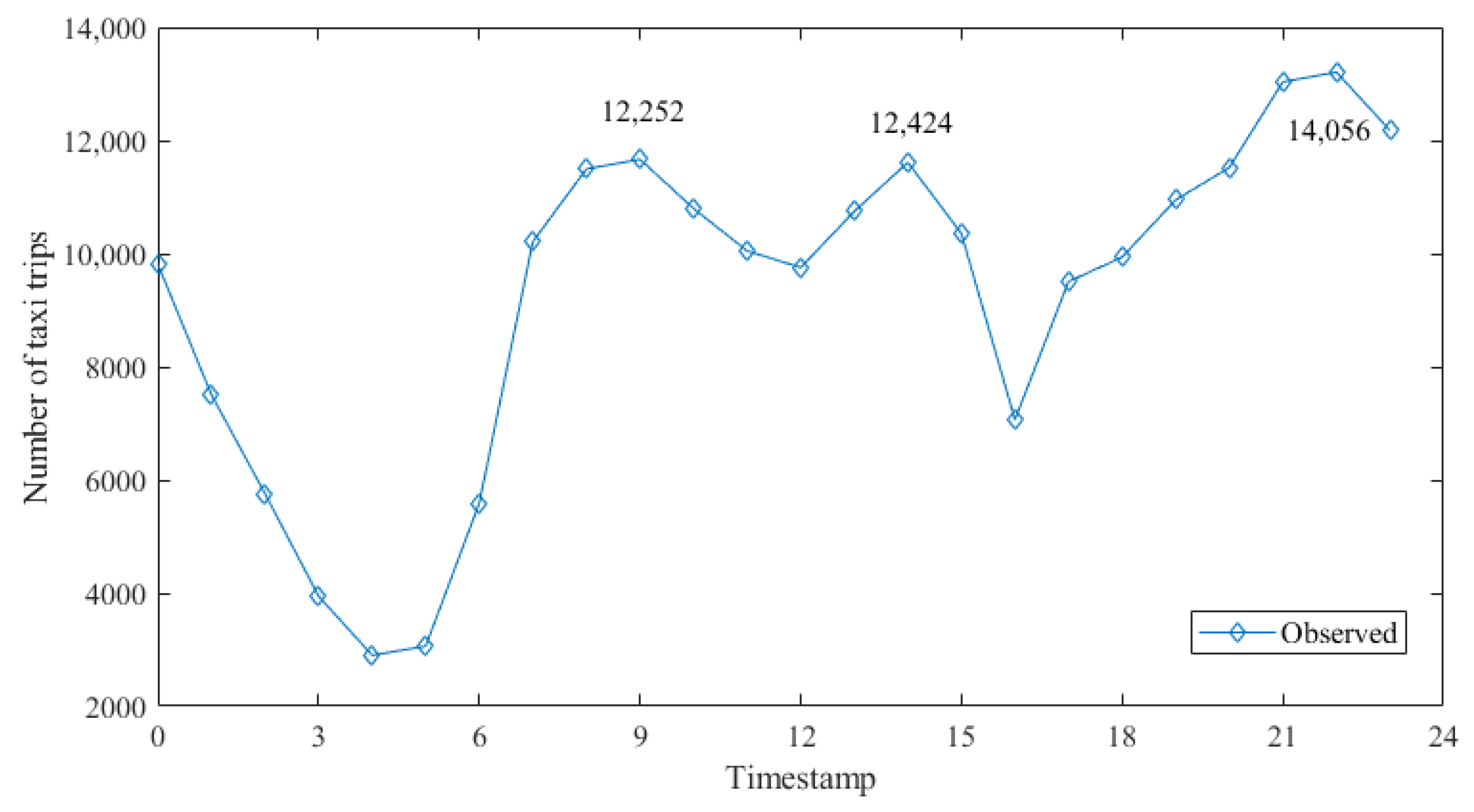
3.1. Taxi Ridership Data

Currently, nearly 6000 taxis operate in the city, generating more than 230,000 daily trips based on observations from November 2015. Due to privacy protection issues, instead of the complete trajectory, only projected coordinates for the pickup and drop-off points were provided. In addition, the data also contained the starting/ending GPS time, driving distance, and total cost. Since trip numbers were stable on a weekly basis, except for special events, and exhibited repetitive patterns within each week, we extracted data for the workdays using one weekday (2nd to 6th November 2015) for further analysis of taxi ridership. We excluded taxi ridership during the weekend due to the variable patterns of travel. After importing trip records into a spatial database, the following recodes were removed:

• Missing coordinates for OD location or location outside the study area.
• Missing trip distance d or d <300 m or d >40 km.
• Missing trip time t or t <1 min or t >4 h.

After applying a process to clean the data, there were 1,113,276 trips in the selected weekdays, and no special events for holidays were reported. Three peak periods were evident (Figure 3), including a morning peak (8:00–10:00), afternoon peak (13:00–15:00), and evening peak (21:00–23:00). The mean number of taxi journeys during peak hours was generally higher than during off-peak hours. As expected, due to the public transport system being unavailable, the evening peak hours contained the highest number of taxi trips. It should be noted that the histogram of the taxi ridership was too skewed to satisfy the normality assumption of the regression model. Thus, a log transformation was usually applied to the ridership data to satisfy the normality of the distribution of the sample mean [11].

Using the pickup time provided in the records, we calculated the mean hourly taxi ridership for all grid cells for the equivalent time period from Monday to Friday. Figure 4 shows the spatial distribution result of pickup points in the study area. Figure 4a represents the aggregation cells of average taxi ridership during the all weekdays. It is obvious that the high density of taxi ridership was concentrated on the main roads in Xiamen Island. There were no taxi data for the southern part of the island occupied by a large mountainous area. With regard to the temporal dimension, Figure 4b–d represents the variability of taxi distribution for three different peak times. Influenced by urban form and functionality, 34 cells were associated with a total ridership of over 60, while the above 200 cells possessed a total ridership of less than 10. The incoherence between cells demonstrates unbalanced taxi ridership in Xiamen Island. The elucidation of the fundamental mechanisms of the urban environment is thus pivotal.

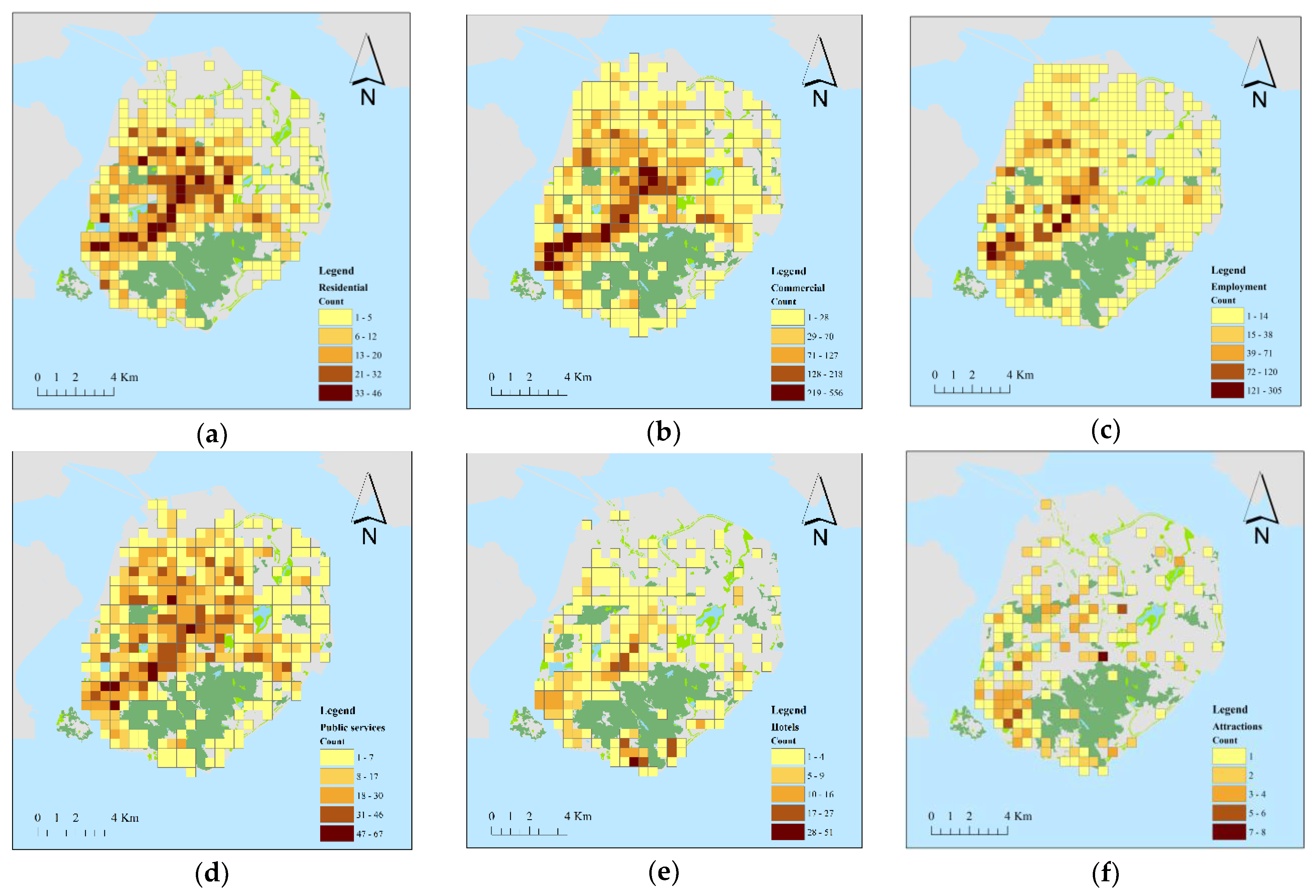
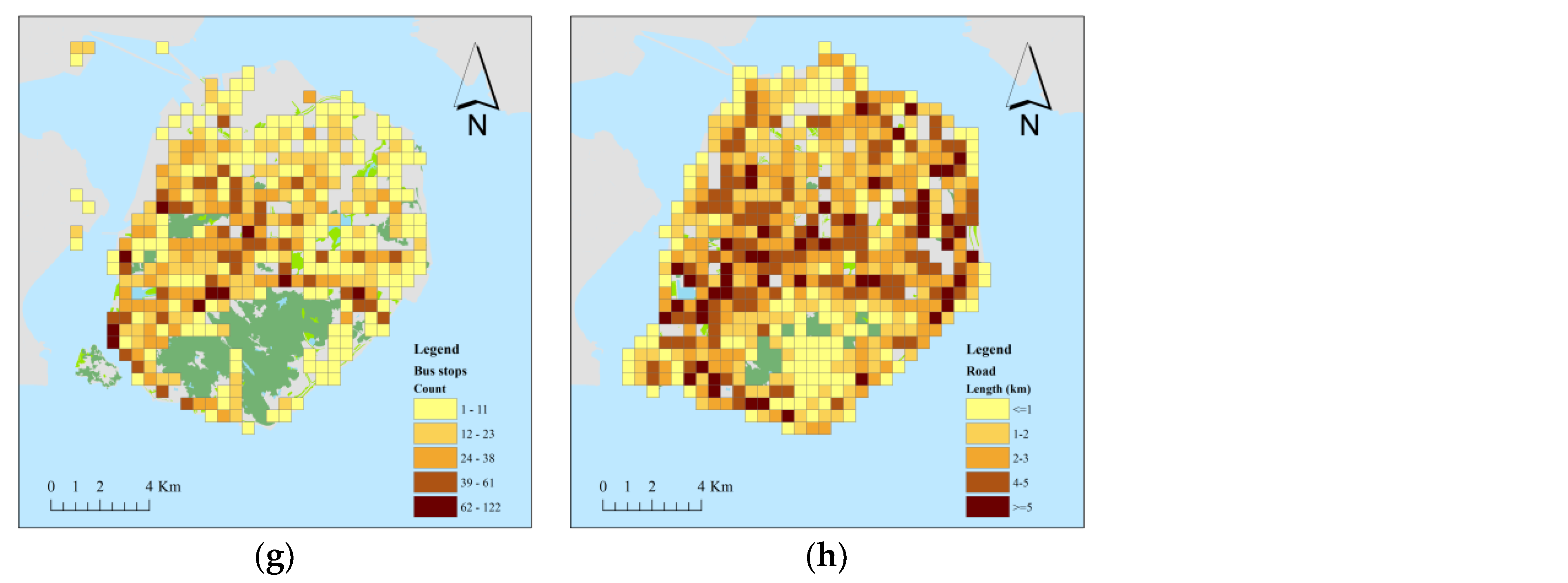
3.2. Urban Environment Assessment

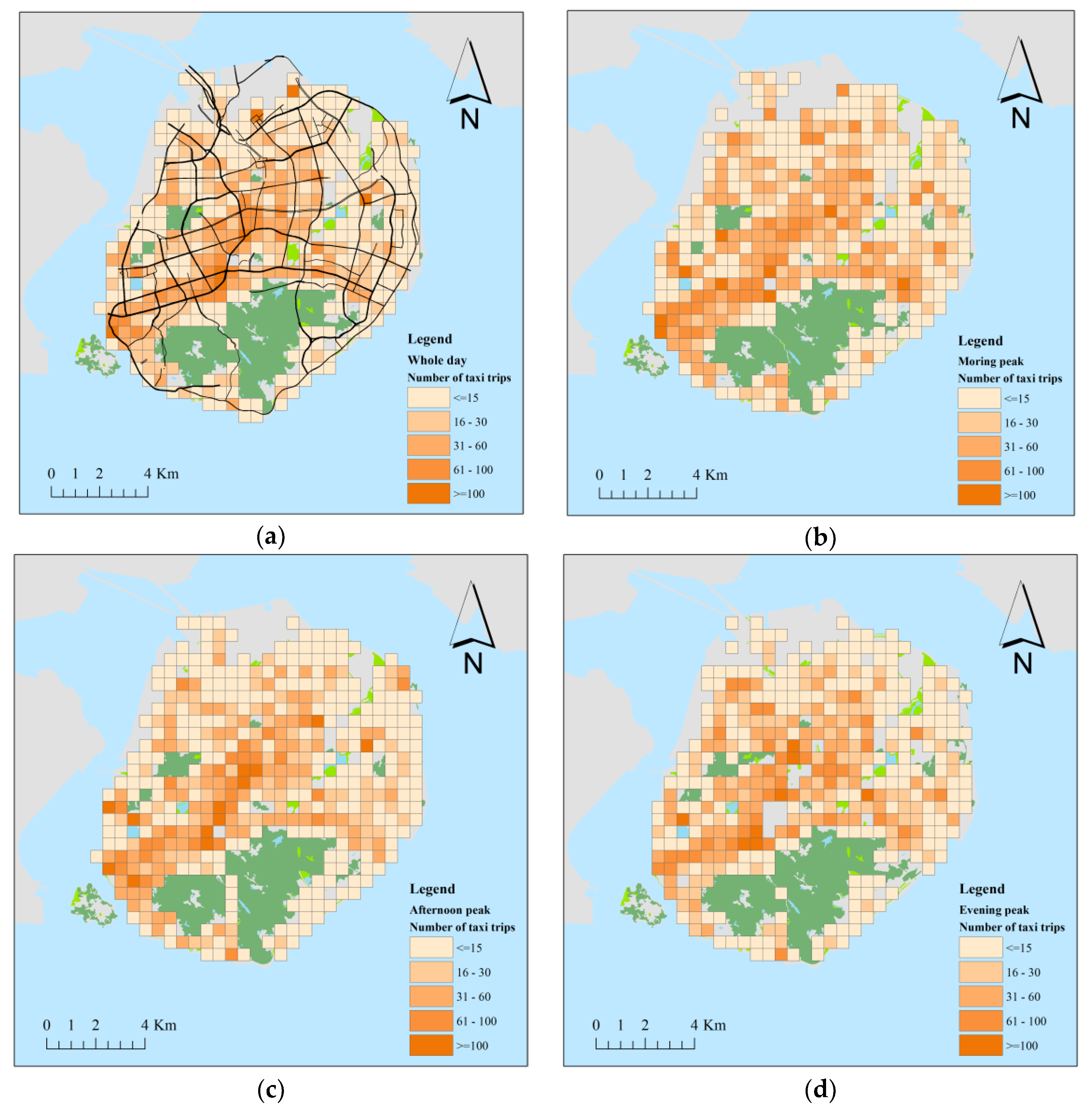
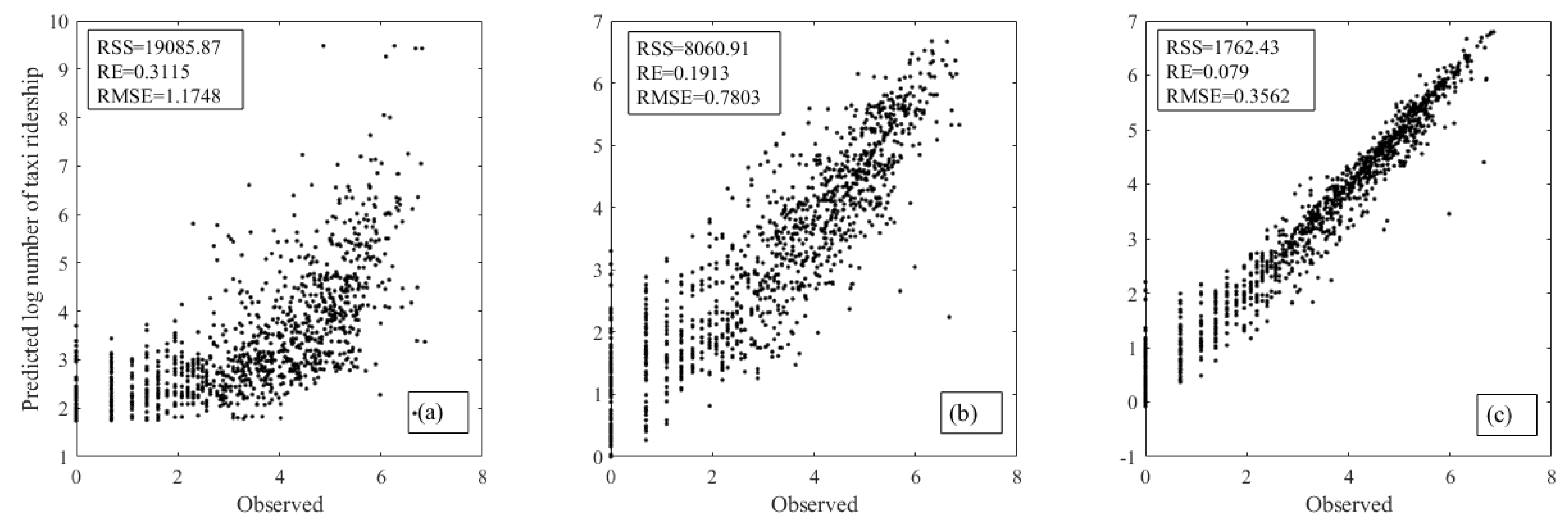
POI data were obtained from Gaode.com; one of the largest Chinese web mapping service applications. Using the zonal statistics tool using ArcGIS toolbox, seven urban environmental factors were produced. The road network was acquired from Open Street Map (OSM, http://www.openstreetmap.org/) to identify the road length of each TAZ. These factors for each grid cell were respectively computed, including residential building number, commercial establishments, and public services facilities, places of employment, attractions, and bus stops. Due to restraints on data acquisition, the area of each POI was not evaluated in this paper. Detailed definitions of the built environment variables are provided in

Table 1. List of explanatory variables.

Type	Variable	Description
Urban environment	Residential	Number of residential records in each cell
	Commercial	Number of retail stores, shopping malls, restaurants and entertainment centres in each cell
	Employment	Number of companies, education and government offices in each cell
	Public service	Number of financial, telecommunication, automobile and medical services in each cell
	Hotel	Number of hotels in each cell
	Attraction	Number of tourist attractions in each cell
Transport	Bus stop	Number of bus stops in each cell
	Road	Length of road in each cell

.

Figure 5a,b respectively illustrate the spatial division of residential and commercial building densities in Xiamen Island. It shows that a high density of buildings was concentrated in the central area of the island and extended south-westward along the main traffic road. Figure 5c,d indicates the spatial distribution density of places of employment and public services. These spatial distributions corroborate those of residential and commercial densities. Bus stops are situated in the central district, while high density areas and roads are distributed across the island.

A multicollinearity issue in the models will cause highly unreliable results, and thus multicollinearity among the variables requires assessment prior to the implementation of the three models. To address this issue, we applied Pearson correlations to calculate the variables in this study.

Table 2. Pearson correlation coefficient for explanatory variables.

	Res.	Com.	Emp.	Public Services	Hotel	Att.	Bus	Road
Residential	1
Commercial	0.752	1
Employment	0.528	0.627	1
Public services	0.757	0.779	0.503	1
Hotel	0.272	0.415	0.372	0.335	1
Attraction	0.194	0.159	0.113	0.209	0.202	1
Bus stop	0.475	0.474	0.373	0.504	0.322	0.188	1
Road	0.150	0.191	0.173	0.154	0.084	0.121	0.274	1

presents the test results for the pairwise correlations between the independent variables. Most of the correlation coefficients were below 0.7. However, the pairwise correlation between the variables for residential and commercial buildings (0.752), residential buildings and public services (0.757), and commercial and public services (0.779) implied the existence of collinearity. As a result, public services and commercial variables can be removed from the model. The remaining six variables were significant at a 0.01 level, indicating that the null hypothesis should be rejected.

4. Model Results

As pointed out earlier in Section 2.2, the measurement units for space and time were usually different. In our case, space distance was measured in meters and time in hours. Both units required harmonization prior to calculating the space–time weighting matrices. We introduce a parameter τ (Equation (6)) to balance the impacts caused by the different spatial and temporal units. This parameter was obtained using a cross-validation procedure in terms of goodness-of-fit. Figure 6 provides the details of parameter selection using 10% random samples. It shows that the optimal parameter of τ was 75.

A 10-fold CV process was carried out in this study to examine models. In particular, we randomly extracted one-fold samples first and implemented all three model fittings with the other nine-fold samples, and then evaluated models’ performance using the isolated one-fold samples. This process was repeated for each of the 10-fold samples. The OLS models were first applied to investigate significant factors that influence urban taxi ridership, and the results are presented in

Table 3. Estimation result for the OLS model.

Variable	Coefficient	t-statistic	t-probability	VIF
Intercept	1.834	20.100	0.000	--
Residential	0.053	10.075	0.000	1.651
Employment	−0.001	−0.317	0.751	1.556
Hotel	0.062	6.122	0.000	1.258
Attraction	−0.032	−0.764	0.444	1.084
Bus stop	0.036	12.943	0.000	1.517
Road	0.216	7.933	0.000	1.125
Diagnostic Information
R2	0.4691
Adjusted R2	0.4662
AIC	110,806.15
RSS	19,085.87

. Taking each sample values separately, this table contains the estimated coefficients for independent variables, and metrics for the goodness of model fit. According to the t-probability abilities, all explanatory variables except employment were statistically significant at the 95% confidence level. According to the adjusted R², with six explanatory variables, only 46.91% of the variance can be explained for the variation of taxi ridership. Based on the coefficient values, many variables showed an intuitive relationship with taxi ridership. In particular, residential area, hotels, bus stops, and road length positively correlated with taxi ridership, whereas attraction density and places of employment negatively correlated with taxi ridership. The negative sign with respect to attraction density implied that under certain circumstances more tourist attractions decreased the number of taxi trips. This counterintuitive result points to a general weakness of the OLS model, that is, its difficulty in explaining independent variables that are homogenous over space and time. Consequently, we suspected that the results from the OLS model were erroneous and we conducted further investigations using the GWR and GTWR models. In addition, the variance inflation factor (VIF) values for the six independent variables ranged from 1.084 to 1.651. All the VIF values were close to one, indicating that the variables have been carefully selected to avoid the multicollinearity issue [11].

The estimated coefficient results from the GWR and GTWR models were incredibly large due to the variation in the urban environment on transit ridership along spatial and temporal scales. To utilize appropriate comparisons, earlier studies recommended the use of several typical values of the estimated coefficients to determine the magnitude of impact of each variable [18]. In the present study, six statistics, including the average value (AVG), minimum value (MIN), maximum value (MAX), lower quartile (LQ), median (MED), and upper quartile (UQ), were selected (

Table 4. Estimation of the GWR model.

Variable	AVG	MIN	MAX	LQ	MED	UQ
Intercept	1.877	0.0100	5.5974	1.1780	1.6947	2.4620
Residential	0.069	−0.4256	1.1324	0.0243	0.0531	0.0905
Employment	0.020	−0.1162	0.5169	−0.0048	0.0020	0.0302
Hotel	0.213	−0.8061	1.8083	0.0970	0.1790	0.2806
Attraction	−0.100	−1.3732	1.5520	−0.3395	0.0958	0.0806
Bus stop	0.044	−0.0537	0.3449	0.0149	0.0343	0.0730
Road	0.177	−0.4226	1.3716	0.0215	0.1560	0.2915
Diagnostic Information
R2	0.7805
Adjusted R2	0.7793
AIC	101,115.35
RSS	8060.91

). The signs of the average coefficients of the variables matched those of the OLS model except employment that converts to positive. The adjusted R² was 0.7805 for the GWR model, which corresponds to a 0.3114 improvement in the goodness-of-fit significance in comparison to the OLS model. Moreover, given the same dataset, the reductions in the AIC and RSS values also prove the superiority of the GWR model over the OLS model.

As discussed earlier, the GWR model can address the existence of spatially non-stationary data, and as such, the calibrated coefficients of independent variables vary in the study area. According to the estimated coefficients of variables, all six variables show a moderate inconsistency, indicating that the effects of these variables might change in space. Taking attraction as an example, the lower quartile value was −0.3395 and the upper quartile value was 0.0806. Compared with the constant negative value (−0.032) in OLS model, this range indicated that the number of attractions might behave as a positive effect for increasing the number of taxi trips at some certain places. We apply the LQ and UQ values to evaluate the variation of variables because they are not affected by distributions of MAX and MIN values. Thus to some extent, they improved the representation of coefficients.

Results of the GTWR models were obtained using the same set of independent variables.

Table 5. Estimation of the GTWR model.

Variable	AVG	MIN	MAX	LQ	MED	UQ
Intercept	1.8463	−3.2832	7.4410	0.8118	1.7029	2.6531
Residential	0.0760	−1.6402	2.4488	0.0102	0.0505	0.1134
Employment	0.0216	−0.4920	1.0506	−0.0087	0.0027	0.0323
Hotel	0.2414	−12.1476	3.7126	0.0695	0.1974	0.3782
Attraction	−0.1390	−4.8221	3.4925	−0.4156	−0.1002	0.1653
Bus stop	0.0460	−0.1327	0.7814	0.0107	0.0385	0.0723
Road	0.1746	−1.8823	3.1798	−0.0358	0.1711	0.3821
Diagnostic Information
R2	0.9527
Adjusted R2	0.9524
AIC	84,026.81
RSS	1762.43

presents the model estimation for the weekday GTWR model. It should be noted that the percentage of explanation of the variance (Adjusted R²) increased from 0.7793 in the GWR model to 0.9524 in GTWR. It revealed that, even if reductions in AIC (from 101,115.35 for GWR to 84,026.81 for GTWR) and RSS were taken into account, the GTWR achieved better performance. The reduction of these values further indicated that GTWR gives a better fit of data than the GWR and OLS models. It should be noted that the coefficients of GTWR model have a wider floating range between the MIN and MAX values than that of the GWR model. We speculate that this is because the GTWR model can deal with both temporal and spatial heterogeneity. More discussion about this issue can be found in Section 5.2.

The results of Table 3, Table 4 and Table 5 on the study area can be visualized in Figure 7. In this figure, we randomly selected 10% of samples for scatter plot and list three accuracy evaluation indicators, including the RSS, RE, and RMSE of OLS, GWR, and GTWR models. It is clear that the GTWR model shows the best performance of model fitting and validation. The value of RSS reach minimum in GTWR for 1762.43, followed by GWR and OLS with a respective value of 8060.91 and 19,085.87. Correspondingly, lower values of RE and RMSE were observed in the GTWR model (RE and RMSE were respectively 0.079 and 0.3562), indicating that with simultaneous temporal weighting, the GTWR model incorporating urban environmental factors can capture the spatiotemporal variability of taxi ridership to a great degree.

The overfitting problem is common in regression models. In order to verify this issue, we randomly selected different proportions of the entire samples for model validation in

Table 6. GTWR model performance in comparison with different sample proportions.

Proportion	100%	70%	50%	30%	10%
R2 (GTWR)	0.9783	0.9803	0.9837	0.9873	0.9389
R2 (GWR)	0.8091	0.8360	0.8379	0.7824	0.7806
R2 (OLS)	0.4699	0.4707	0.4890	0.4523	0.4478

. In the table, it was evident that a good transferability of the GTWR model because of the model’s performance did not significantly deteriorate.

5. Discussion

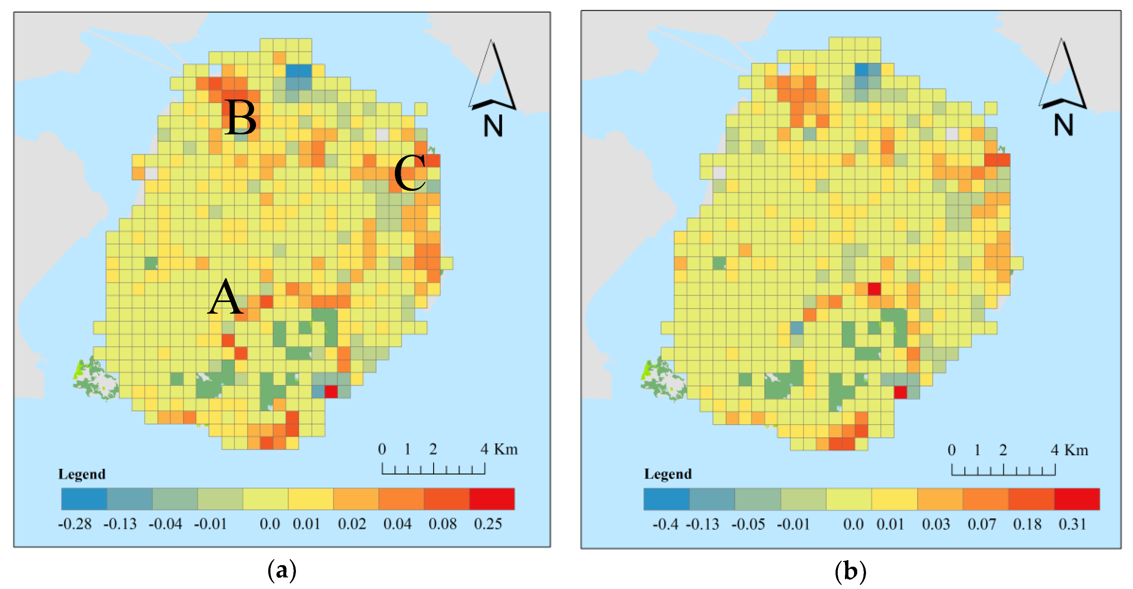
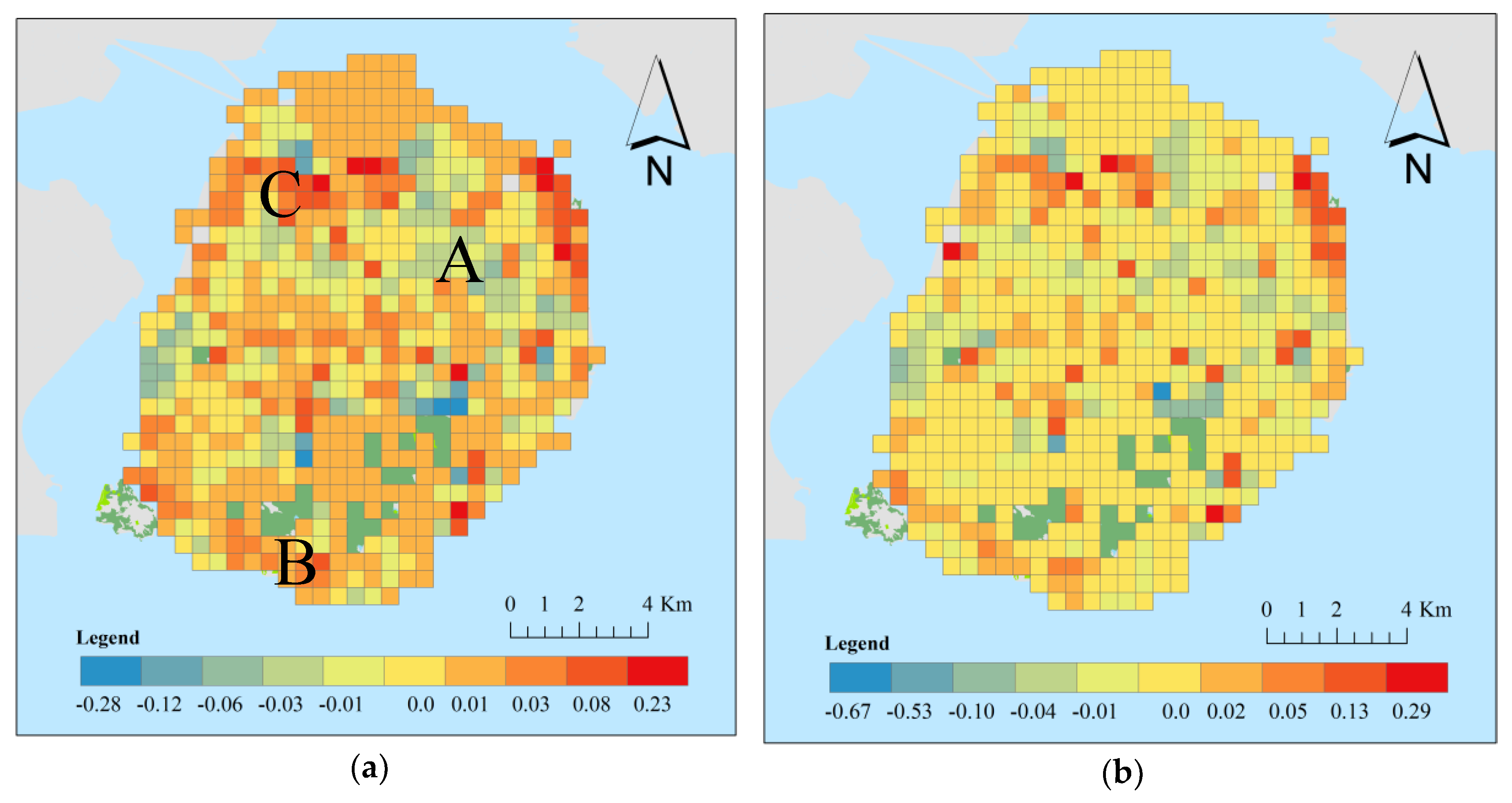
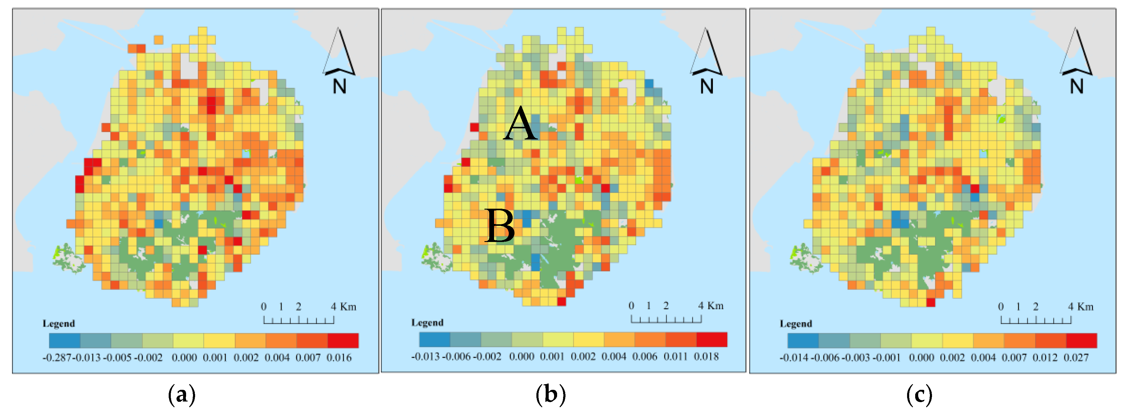
5.1. Spatial Variations of the Coefficients

In contrast to global models, a significant benefit of GWR-based models is that local coefficients, which indicate spatial relationships, can deliver a detailed account of how the explanatory variables differ locally. With the help of GIS technology, coefficients can be grouped into several intervals, and different colors can be used to render the spatial effects of the urban environment variable on taxi ridership [26]. Taking residential variables for example, the coefficient of residential density (0.053) in the OLS model is observed to positively correlate with taxi ridership. However, results from the GWR and GTWR models reveal that the actual influence of residential density may be either negative or positive, depending mainly on the underlying geographical location and temporal period.

Based on the GWR and GTWR model results, cells with different timestamps but the same coordinates were aggregated into one individual cell by calculating mean values. After this processing step, Figure 8 visualizes the spatial distribution of the average coefficients for residential density during entire weekdays. The spatial distribution of GTR and GTWR models are similar. It can be seen that instead of region A, which has the highest density of residential buildings, the higher values of the coefficients were located in region B (0.33) and C (0.16). Since both regions are newly developed zones with less public transit system coverage, the discrepancy reflects the imbalance between urban functionality and traffic resources. According to the spatial distribution of taxi ridership from Figure 4, another possible explanation is that, based on their past habits and experiences, taxi drivers prefer to carry out their business in core areas. In their opinion, it is costly to pick up passengers in places distant from core areas.

Similar spatial pattern analysis can also be adopted for the density of attractions. In the OLS model, this variable’s specification is observed to be negatively correlated with ridership (−0.032). Figure 9 visualizes the spatial distribution of the coefficients for attraction density during weekdays. It can be seen that coefficients of attraction density in most of regions are positive, such as regions B and C. It means that the number of tourists requesting taxi rides is reinforced by the number of attractions in these areas. This is contradicted by the fact that there is a negative linear correlation in the OLS model. In fact, positive coefficients of the GTWR model indicate that many tourists are concentrated in these areas, thereby increasing the chance of hailing a taxicab. The negative coefficients in region A imply a non-linear relationship, i.e., that taxi ridership does not scale proportionally to the square of attractions.

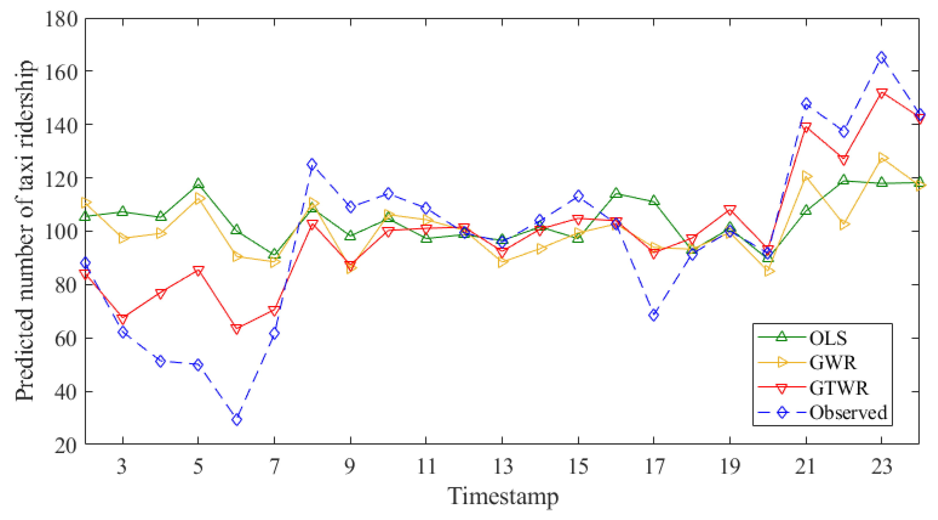
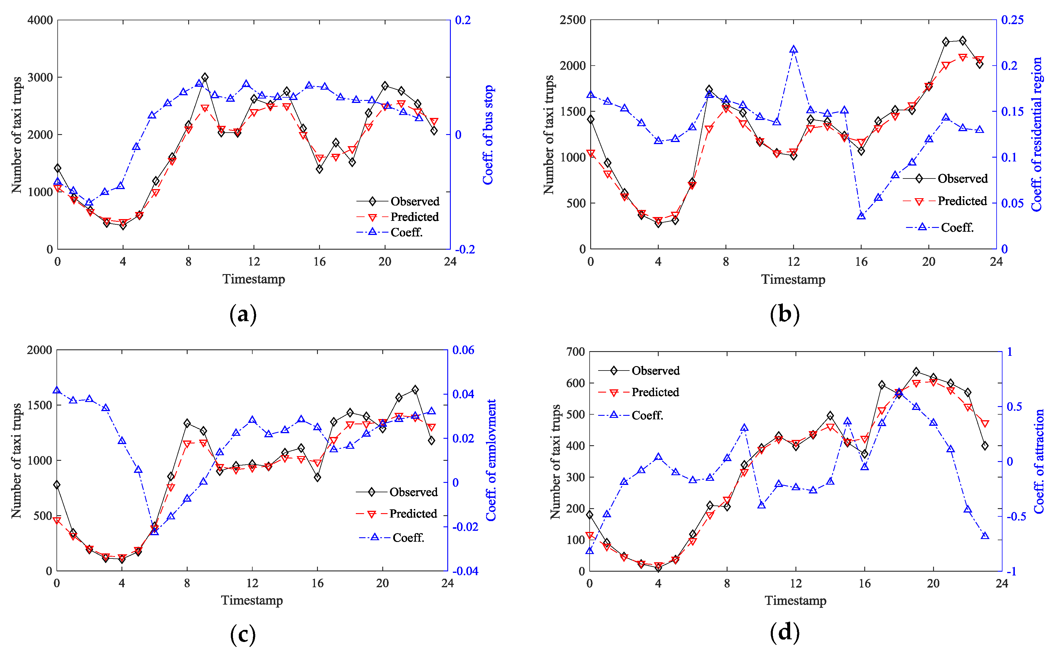
5.2. Temporal Variations of the Coefficients

The enhancement of GTWR can be attributed to integrating the temporal dimension into the conventional GWR model. Thus, from the GTWR model results, we can consequently attain the time series of the hourly predictions and coefficients. Figure 10 presents the predicted number of taxi trips on Xiamen Island during weekdays. It shows that either the OLS model or GWR model lacks the ability to reflect temporal variations in the number of taxi trips. On the contrary, results of GTWR can accurately reflect the dynamic trend of the variation in taxi trips, which initially decrease towards midnight, exhibit a rapid increase from 6:00 to 9:00, and then fluctuate until the end of the day. The GTWR model can explain 97.83% of the actual change in taxi trips, indicating that certain details related to the dramatic fluctuations in taxi ridership are fully captured in different periods. The time with the biggest difference between the predicted and observed value is between 4:00–6:00 a.m. One possible reason is that there are insufficient taxi records in this period, which cause model underfitting.

Taxi passenger journeys, the attributes of which can be explained in a spatial and temporal framework, are a significant component of city transit during weekdays. To evaluate the extent to which the impact of urban environmental variables on taxi ridership is time-dependent, the mean coefficient values for three peak periods were provided (

Table 7. Average coefficients across the different peak periods.

Variable	Period
	Morning Peak	Afternoon Peak	Evening Peak
Residential	0.048	0.102	0.121
Employment	0.136	0.050	0.046
Hotel	0.093	0.013	0.057
Attraction	−0.294	−0.155	−0.215
Bus stop	0.054	0.053	0.045
Road	0.008	0.173	0.230

). In general, during the three peak periods, except for the density of attractions, the average coefficients of the environmental variables were positive with respect to the increment of taxi ridership. As a result of attractions closing times, the density of attractions coefficients during evening peak hours had a greater negative influence on taxi ridership than at daytime hours. The residential building factor positively influenced transit ridership at all peaks, but increased progressively over time. In contrast, the average effect of places of employment density on ridership became more negative over time. This finding indicates that the daily travel cycle of people leads to the inverse correlation between residential places and places of work.

As expected, the average coefficient of bus stop and road density were positive during all three periods. This result may be attributed to passenger’s habits of taking taxis in places with a high density of roads or bus stops, where it is easier to hail a taxi. However, there is competition among travel modes, and highly dense roads are often accompanied by frequent congestion. To be specific, Figure 11 further elaborates the spatial distribution of the coefficients of road density at three different peaks. In general, it can be seen that road density in the eastern part of the island has more positive effects for the number of taxi trips than the western part. The imbalance might be contributed to the fact that several bridges and tunnels, leading to the outside of the island, are located in the western part. As a result, traffic jams are frequent, thereby reducing the positive effects of road density for the number of taxi trips. For example, the coefficients of road density in region A declined over time, reflecting that taxi drivers were unwilling to serve areas where the high density of roads might cause traffic congestion issues. Furthermore, the coefficients of region B presented the same decline as region A. The increasing negative effects of road density may be due to Xiamen’s railway station being located here. Most passengers were willing to take bus instead of taxi based on cost.

To further assess the explanatory capacity of the GTWR model at both spatial and temporal scales, four typical regions were carefully selected, including the railway station, high-density employment areas, residential areas, and scenic areas. The locations of these areas and their corresponding grid cells are shown in Figure 12. The coefficients of explanatory variables had been calculated using the GTWR model for each cell, therefore their median and average values were aggregated to describe coefficients of the whole region.

Figure 11a presents the predicted results of taxi ridership, consisting of four grid cells covering the railway station. The flux in taxi ridership at the Xiamen railway station showed a double-peak distribution. Moreover, since the railway station connects the internal and external traffic of city, it is important to analyze which means of transportation people are likely to take. In this context, it is either bus or taxi. Figure 13a thus indicates that, during bus operating hours (7:00–22:00), the temporal variability in the coefficients of bus stops demonstrated a positive pattern to that of taxi ridership. This suggests that a larger number of bus stops actually increased taxi ridership. On the contrary, during the night, the coefficient was negative, indicating that the presence of bus stops decreased taxi demand. This result suggests the existence of a competitive relationship between buses and taxis in the railway station area. Especially after 16:00, when taxi drivers are changing shifts and traffic become more jammed, passengers prefer to take the bus. This makes the coefficients of bus stop density more negative.

Figure 13b presents the GTWR modelling results for an area called Lian-Qian, which has a high density of residential buildings. Both the variability in taxi ridership and the associated coefficients in this residential area indicate a three-peak distribution. At 7:00, the first peak of the coefficients of residential areas occurs, as taxis were frequently used by people to get to their workplaces faster and more conveniently. The second one had the highest coefficient value during midday, proving that passengers were likely to take a taxi away from home for lunch or work. The last peak happened after 20:00, indicating people might leave home to other places for activities, such as shopping and socializing.

The area called Software-Park-Phase-II represents the core business district in Xiamen and contains an abundance of information technology companies. The comparison between the predicted value obtained from the GTWR model and the observed value in this area is indicated in Figure 13c, as well as the temporal fluctuation of the coefficients for employment places. It was evident that the positive coefficient for places of employment started increasing at 8:00. In an area hosting an abundance of places of employment, the corroboration between taxi ridership and the coefficient, established temporally-dependent influences of places of employment on taxi ridership.

The Zeng-Cuo-An area, which constitutes a classic tourist district in Xiamen City, was denoted as an example of an attraction-oriented area. Tourists are greatly attracted to this area due to its different styles of regional architecture. The time series of the predicted value based on the GTWR model and the observed value is described in Figure 13d. It demonstrates that taxi ridership escalates sharply at the beginning of the service time (8:00). Ridership starts to increase at 14:00, then peaks at 19:00, where it remains for the remainder of the service period. The coefficients of attraction present a similar trend as ridership at the beginning, especially with a sharp decline after 21:00. This result shows the typical fluctuation of ridership for an area with tourist attractions.

6. Conclusions

It is important that taxi ridership is affected by both time and space. This study aimed to evaluate the association between taxi ridership and urban environment, using the spatiotemporal regression model, GTWR. To establish the spatiotemporal impact of the built environment on taxi ridership in Xiamen City, the efficacy of the GTWR model was assessed based on a week of taxi OD data, and an assortment of POI data. As such, this study examines the influence of urban environmental factors on hourly taxi ridership over both space and time. The significant advantage of the GTWR model is that it can consider temporal variations. In comparison with conventional OLS and GWR models, the experimental findings demonstrate that the GTWR model exhibits increased adaptability. As it is a local spatiotemporal model, the temporal variations of the coefficients derived from it can be further visualized and assessed for determining temporally-dependent vacillations in the coefficients.

Particularly, at the grid unit scale, the temporal heterogeneity of the coefficients is highlighted as a major factor determining taxi ridership. The GTWR model can concurrently combine spatial and temporal non-stationarities into ridership assessment. Elucidating the causes of transit ridership allows for a more precise estimation than conventional models in terms of goodness-of-fit. By investigating the coefficients’ spatial and temporal distributions, the time-dependent effects of four different representative regions on taxi ridership were further confirmed. Using the results of the GTWR model, the urban planning and transit management departments can improve targeted policies to increase the value of transit services.

However, there is still room for improving this study. For instance, model development can consider road capacity and traffic congestion related data. In addition, in the present version of GTWR, Euclidean distance is used to combine temporal and spatial distances. Advanced and nonlinear weighting algorithms, such as geographical distance and seasonal variations [27], might be more appropriate for reality, and should be developed for further study. To evaluate the model’s functionality, a sensitivity analysis of varying time units can also be incorporated.

References

1. King, D.A.; Peters, J.R.; Daus, M.W. Taxicabs for Improved Urban Mobility: Are We Missing an Opportunity? Presented at the Transportation Research Board 91st Annual Meeting, Washington, DC, USA, 22–26 January 2012. [Google Scholar]
2. Nie, Y.M. How can the taxi industry survive the tide of ridesourcing? Evidence from Shenzhen, China. Transp. Res. Part C Emerg. Technol. 2017, 79, 242–256. [Google Scholar] [CrossRef]
3. Chakraborty, A.; Mishra, S. Land use and transit ridership connections: Implications for state-level planning agencies. Land Use Policy 2013, 30, 458–469. [Google Scholar] [CrossRef]
4. Taylor, B.D.; Miller, D.; Iseki, H.; Fink, C. Nature and/or nurture? Analyzing the determinants of transit ridership across us urbanized areas. Transp. Res. Part A Policy Pract. 2009, 43, 60–77. [Google Scholar] [CrossRef]
5. Ma, X.; Zhang, J.; Ding, C.; Wang, Y. A geographically and temporally weighted regression model to explore the spatiotemporal influence of built environment on transit ridership. Comput. Environ. Urban Syst. 2018, 70, 113–124. [Google Scholar] [CrossRef]
6. Pinelli, F.; Nair, R.; Calabrese, F.; Berlingerio, M.; Di Lorenzo, G.; Sbodio, M.L. Data-driven transit network design from mobile phone trajectories. IEEE Trans. Intell. Transp. Syst. 2016, 17, 1724–1733. [Google Scholar] [CrossRef]
7. Yang, Z.; Franz, M.L.; Zhu, S.; Mahmoudi, J.; Nasri, A.; Zhang, L. Analysis of Washington, DC taxi demand using GPS and land-use data. J. Transp. Geogr. 2018, 66, 35–44. [Google Scholar] [CrossRef]
8. Liu, Y.; Wang, F.; Xiao, Y.; Gao, S. Urban land uses and traffic ‘source-sink areas’: Evidence from gps-enabled taxi data in Shanghai. Landsc. Urban Plan. 2012, 106, 73–87. [Google Scholar] [CrossRef]
9. Zhao, J.; Qu, Q.; Zhang, F.; Xu, C.; Liu, S. Spatio-temporal analysis of passenger travel patterns in massive smart card data. IEEE Trans. Intell. Transp. Syst. 2017, 18, 3135–3146. [Google Scholar] [CrossRef]
10. Davis, L.W. The effect of driving restrictions on air quality in Mexico city. J. Political Econ. 2008, 116, 38–81. [Google Scholar] [CrossRef]
11. Qian, X.; Ukkusuri, S.V. Exploring Spatial Variation of Urban Taxi Ridership Using Geographically Weighted Regression. Presented at the 94th Annual Meeting of the Transportation Research Board, Washington, DC, USA, 11–15 January 2015. [Google Scholar]
12. O’Sullivan, D. Geographically Weighted Regression: The Analysis of Spatially Varying Relationships; Fotheringham, A.S., Brunsdon, C., Charlton, M., Eds.; The Ohio State University: Columbus, OH, USA, 2003; Volume 35, pp. 272–275. [Google Scholar]
13. Cardozo, O.D.; García-Palomares, J.C.; Gutiérrez, J. Application of geographically weighted regression to the direct forecasting of transit ridership at station-level. Appl. Geogr. 2012, 34, 548–558. [Google Scholar] [CrossRef]
14. Chow, L.F.; Zhao, F.; Liu, X.; Li, M.T.; Ubaka, I. Transit ridership model based on geographically weighted regression. Transp. Res. Rec. J. Transp. Res. Board 2006, 1972, 105–114. [Google Scholar] [CrossRef]
15. Chiou, Y.-C.; Jou, R.-C.; Yang, C.-H. Factors affecting public transportation usage rate: Geographically weighted regression. Transp. Res. Part A Policy Pract. 2015, 78, 161–177. [Google Scholar] [CrossRef]
16. Chen, C.; Varley, D.; Chen, J. What affects transit ridership? A dynamic analysis involving multiple factors, lags and asymmetric behaviour. Urban Stud. 2011, 48, 1893–1908. [Google Scholar] [CrossRef]
17. Ma, T.; Motta, G.; Liu, K. Delivering real-time information services on public transit: A framework. IEEE Trans. Intell. Transp. Syst. 2017, 18, 2642–2656. [Google Scholar] [CrossRef]
18. Huang, B.; Wu, B.; Barry, M. Geographically and temporally weighted regression for modeling spatio-temporal variation in house prices. Int. J. Geogr. Inf. Sci. 2010, 24, 383–401. [Google Scholar] [CrossRef]
19. Wu, B.; Li, R.; Huang, B. A geographically and temporally weighted autoregressive model with application to housing prices. Int. J. Geogr. Inf. Sci. 2014, 28, 1186–1204. [Google Scholar] [CrossRef]
20. Fotheringham, A.S.; Crespo, R.; Yao, J. Geographical and temporal weighted regression (GTWR). Geogr. Anal. 2015, 47, 431–452. [Google Scholar] [CrossRef]
21. Bai, Y.; Wu, L.; Qin, K.; Zhang, Y.; Shen, Y.; Zhou, Y. A geographically and temporally weighted regression model for ground-level PM2. 5 estimation from satellite-derived 500 m resolution AOD. Remote Sens. 2016, 8, 262. [Google Scholar] [CrossRef]
22. Guo, Y.; Tang, Q.; Gong, D.-Y.; Zhang, Z. Estimating ground-level pm2. 5 concentrations in beijing using a satellite-based geographically and temporally weighted regression model. Remote Sens. Environ. 2017, 198, 140–149. [Google Scholar] [CrossRef]
23. Chu, H.-J.; Kong, S.-J.; Chang, C.-H. Spatio-temporal water quality mapping from satellite images using geographically and temporally weighted regression. Int. J. Appl. Earth Obs. Geoinf. 2018, 65, 1–11. [Google Scholar] [CrossRef]
24. Liu, Y.; Lam, K.-F.; Wu, J.T.; Lam, T.T.-Y. Geographically weighted temporally correlated logistic regression model. Sci. Rep. 2018, 8, 1417. [Google Scholar] [CrossRef] [PubMed] [Green Version]
25. Peruggia, M. Model selection and multimodel inference: A practical information-theoretic approach (2nd ed.).(telegraphic reviews)(book review). J. Wildl. Manag. 2002, 67, 175–196. [Google Scholar]
26. Zhan, X.; Qian, X.; Ukkusuri, S.V. A graph-based approach to measuring the efficiency of an urban taxi service system. IEEE Trans. Intell. Transp. Syst. 2016, 17, 2479–2489. [Google Scholar] [CrossRef]
27. Du, Z.; Wu, S.; Zhang, F.; Liu, R.; Zhou, Y. Extending geographically and temporally weighted regression to account for both spatiotemporal heterogeneity and seasonal variations in coastal seas. Ecol. Inform. 2018, 43, 185–199. [Google Scholar] [CrossRef]
Figure 1. Flowchart of the proposed method for estimating hourly taxi trips on a 500 × 500 m2 grid unit.
Ijgi 08 00023 g001
Figure 2. Location and grid-based segmentation of Xiamen Island.
Ijgi 08 00023 g002
Figure 3. Hourly average taxi ridership of Xiamen Island.
Ijgi 08 00023 g003
Figure 4. Spatial distribution of taxi ridership at different periods. (a) Whole day; (b) morning peak; (c) afternoon peak; and (d) evening peak.
Ijgi 08 00023 g004
Figure 5. Spatial distribution of different explanatory variables. (a) Residential; (b) commercial; (c) employment; (d) public services; (e) hotels; (f) attractions; (g) bus stops; and (h) road density.
Ijgi 08 00023 g005aIjgi 08 00023 g005b
Figure 6. The parameter selection for the GTWR model.
Ijgi 08 00023 g006
Figure 7. Scatter plots for model fitting and cross validation. (a) OLS; (b) GWR; and (c) GTWR.
Ijgi 08 00023 g007
Figure 8. Spatial distribution of the coefficients of ‘residential density’. (a) GWR; and (b) GTWR. Region A has the highest density of residential buildings. Regions B and C are two newly developed zones.
Ijgi 08 00023 g008
Figure 9. Spatial distribution of the coefficients of ‘attraction density’ (quantified by natural breaks style). (a) GWR; and (b) GTWR. Region A has negative coefficients of ‘attraction density’; Regions B and C have positive coefficients of ‘attraction density’.
Ijgi 08 00023 g009
Figure 10. Temporal variations in the predicted and observed values.
Ijgi 08 00023 g010
Figure 11. Spatial and temporal distribution of the average coefficient for the “road length” variable at three peaks. (a) Moring peak; (b) afternoon peak; and (c) evening peak. Region A represents high density of road; Region B represents railway station.
Ijgi 08 00023 g011
Figure 12. Location of four representative regions.
Ijgi 08 00023 g012
Figure 13. Temporal variation in taxi ridership and coefficients of explanatory variables at four selected regions based on the GTWR model. (a) Railway station; (b) high density of the residential buildings region; (c) high density of the region comprising places of employment; and (d) high density at attractions region.
Ijgi 08 00023 g013