Shoreline Detection using Optical Remote Sensing: A Review


1
Laboratoire d’Electronique Informatique Télécommunication et Energies Renouvelables, Université Gaston Berger, 32000 Saint-Louis, Sénégal
2
INSA Rennes, CNRS, IETR (Institut d’Electronique et de Télécommunication de Rennes), Univ Rennes, UMR 6164, F-35000 Rennes, France
*
Author to whom correspondence should be addressed.
ISPRS Int. J. Geo-Inf. 2019, 8(2), 75; https://0-doi-org.brum.beds.ac.uk/10.3390/ijgi8020075
Submission received: 30 October 2018
/
Revised: 20 December 2018
/
Accepted: 20 January 2019
/
Published: 5 February 2019
(This article belongs to the Special Issue Natural Hazards and Geospatial Information)
Abstract
:With coastal erosion and the increased interest in beach monitoring, there is a greater need for evaluation of the shoreline detection methods. Some studies have been conducted to produce state of the art reviews on shoreline definition and detection. It should be noted that with the development of remote sensing, shoreline detection is mainly achieved by image processing. Thus, it is important to evaluate the different image processing approaches used for shoreline detection. This paper presents a state of the art review on image processing methods used for shoreline detection in remote sensing. It starts with a review of different key concepts that can be used for shoreline detection. Then, the applied fundamental image processing methods are shown before a comparative analysis of these methods. A significant outcome of this study will provide practical insights into shoreline detection.
1. Introduction
It is estimated that there are about 504,000 km of shoreline worldwide, and more than 50% of the world’s population lives within 100 km of the sea [1]. Detecting and monitoring shorelines are consequently of significant economic and social importance, especially if we know that climate change has devastating effects on coastal areas. The shoreline marks the transition between land and sea. Ideally, it is defined as the physical interface of land and water [2]. In some references, the shoreline is expressed as an intersection of coastal land and water surface showing water edge movements as the tides rise and fall [3,4]. In fact, the shoreline is flexible depending on sea level, swell, tides and near-shore currents.
For having a good shoreline detection method, it is necessary to evaluate the existing ones, to know their drawbacks so that we will be able to propose better approaches. Shoreline detection can be achieved using different processes.
Mapping the seabed using acoustic waves such as sonar is currently the only technique that can be used without depth limitation. However, swell conditions and tidal currents can make embedded operations difficult to realize.
Terrestrial surveys can be achieved using landmarks, Global Positioning System (GPS), terrestrial Light Detection And Ranging (LiDAR) or tridimensional (3D) scanners [5]. In general, in situ measurements are difficult to achieve. In this case, other survey methods such as remote sensing are recommended [6].
Remote sensing is the technique of obtaining information about objects or areas from a distance, typically from aircraft or satellites [7]. It is increasingly used in coastal monitoring insofar as it contributes to the fullness of the radiometric information and allows automated or semi-automated extraction of the shoreline by image processing.
To analyse coastal change, a shoreline indicator is required. Because of the dynamic nature of this borderline, the chosen indicator needs to take into account the shoreline in a spatiotemporal sense and must consider the dependency of this variability on the time scale [8].
The rest of this paper shows a state of the art review on shoreline detection methods used in remote sensing.
A compilation of the different shoreline indicators that have been reported in the literature is provided. Then, a summary of shoreline detection approaches in remote sensing is proposed, extending from image pre-processing to segmentation and edge detection.
2. Coastline Indicators
For coastal management purposes, it is necessary to know the evolution of the shoreline according to the associated time scale. In order to analyse these changes, a definition of the shoreline must be given. The definition of the shoreline that theoretically is supposed to represent the linear boundary between the maritime and land domains is very challenging because of the wide variety of indicators (key) that can be based on geomorphologic aspect, tidal level, or the configuration of the vegetation, among others [9].
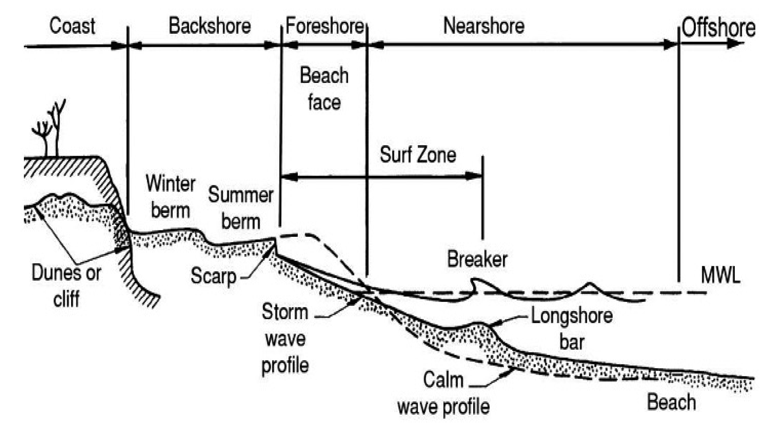
To understand coastline detection methods, it is first necessary to know the organization of the coastal environment. A typical beach profile is represented in Figure 1.
Coastal environments are similar in composition and shape. As shown in Figure 1, four general areas can be defined in a typical beach profile; they extend from the cliff or dunes to the end of the nearshore. Readers are referred to [10,11] for more details of beach profile organization.
This profile can change from one coast to another. For this reason, there is no indicator that can be used for all types of coast; functional indicators depend on the coast profile and the monitoring objectives.
Coastline indicators must have the ability to represent schematically but correctly the overall coastal state from the point of view of its sedimentary evolution [12].
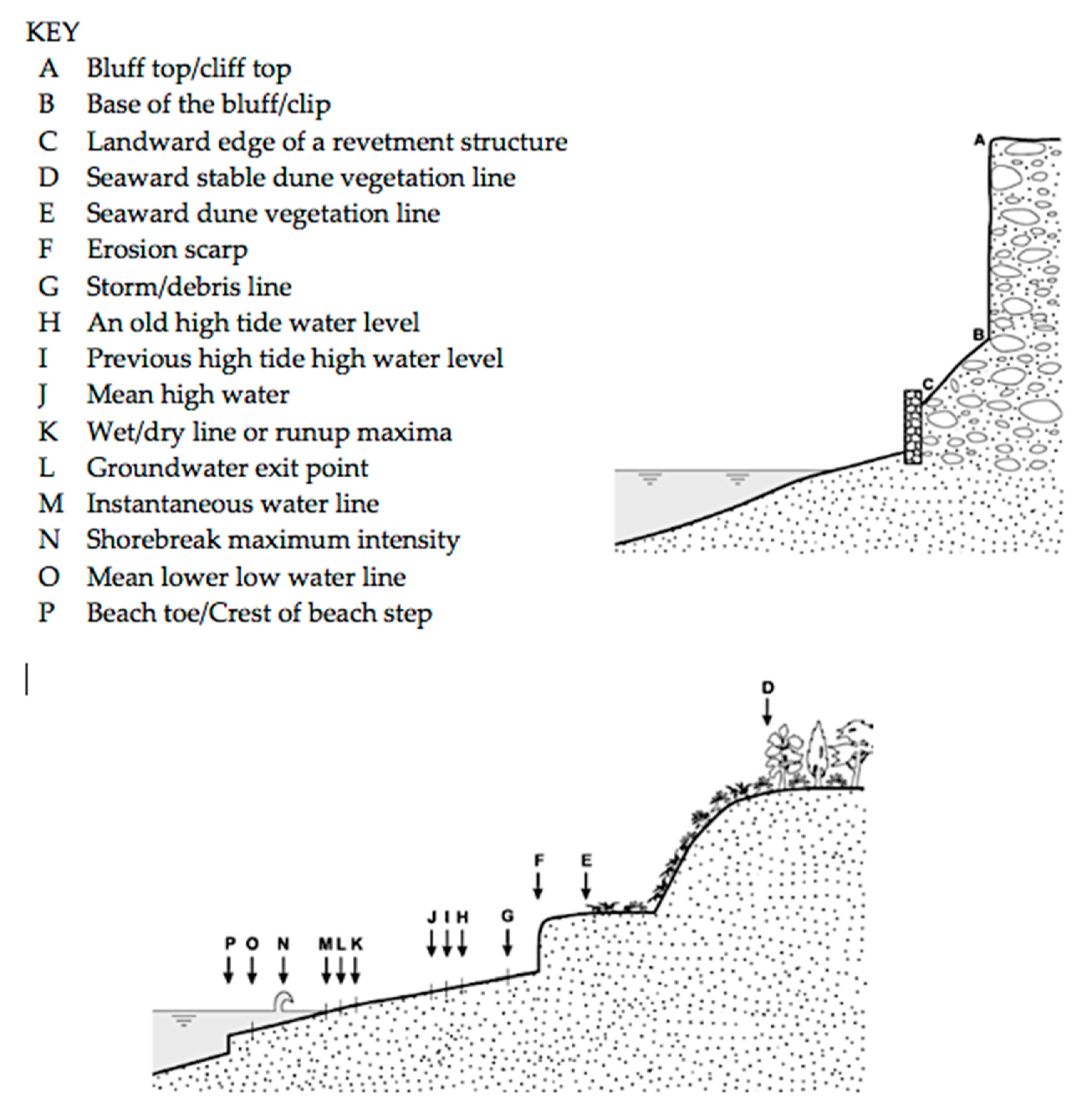
Boak and Turner [8] listed 45 coastline indicators used around the world for coastal monitoring studies. A sketch of the spatial relationship between the most commonly used shoreline indicators is shown in Figure 2. A compilation of these indicators, their description and some references where they are used are given in Table 1, Table 2, Table 3, Table 4 and Table 5. The different kind of indicators represented in this table are organized into seven types: geomorphological reference lines, vegetation limits, instant tidal levels and wetting limits, tidal data, beach contours and storm lines. Each of these types of indicators relates to different indicators that have been used for coastal detection and monitoring.
Detecting the different indicators, shown in the table above, allows coastal monitoring. These indicators should be able to show the environmental modification in the beach area, but they should not be so sensitive to fluctuations in local conditions.
The precision of these indicators depends on the quality of the material, the working conditions and the experience of the operator. Therefore, this precision can vary from one operator to another, but also for the same operator, several results are possible depending on the working conditions. A good way of monitoring these indicators is the use of satellite remote sensing. There is a wide range of satellites whose products can be successfully used for coastal science, and particularly for shoreline detection using automated or semi-automated image processing techniques.
Due to the large range of shoreline indicators, an assortment of image processing tools has been used for shoreline detection. Satellite images are pre-processed in order to produce images which can be integrated into an image processing software for segmentation purposes to detect the shoreline. The following section focuses on the pre-processing techniques.
3. Pre-Processing
Pre-processing methods can be grouped into two kinds, which are noise reduction and image correction. Irrespective of the processes used in a shoreline detection method, it naturally begins with preliminary steps that aim to reduce noise and improve image quality. The quality of a detected shoreline partially depends on the quality of the pre-processing methods applied. By using a pre-processing method that is better adapted to the data set, it is possible to improve the detection result. For a better recognition of the shoreline, it is crucial to reduce noise while preserving edge information. For this reason, adaptive filters, such as the median filter [97], are widely used. They are particularly suitable when the noise is composed of thin lines or isolated points, which are scattered in the image.
The median filter replaces each pixel in the image with the median of those values within the moving kernel. It is always applicable to optical images, as well as LiDAR data [98].
There are multiple types of median filters: Progressive Switching Median Filter, Fuzzy Switching Median Filter, Adaptive Median Filter, Simple Adaptive Median filter [99].
The use of a median filter window smoothens the image while enhancing the edges because some pixels have high grey-level values compared to their neighbours. It is effective in removing white noise, while preserving sharp shoreline edges.
The Lee sigma filter replaces each pixel with the mean of all diagonal values in the moving kernel that fall within the designated standard deviation range, in which the pixels beyond the standard deviation range are regarded as speckle-contaminated and hence are not used to calculate the mean. It takes into account, for estimation of local statistics, only the pixels within a certain range of radiometric values [100].
The Frost filter has the advantage of smoothing homogeneous areas, and preserving edge and transition lines. However, the micro strokes are also smoothed [101].
Noise reduction is an important task in shoreline detection; it allows improving image quality, which contributes to a better detection of the shoreline. However, it is not the on-off pre-processing step applied to satellite images. In the case of a multispectral analysis, it is necessary to perform radiometric and geometric corrections. To minimize the effects of weathering on the radiometric values generated by interpolation during the geometric correction, radiometric corrections must precede geometric corrections [102]. Geometric corrections can be of two kinds; rectification and georeferencing [103]. The rectification is an oblique image correction in order to obtain a vertical image corrected for all or most strains inherent in the shot and distortion produced by the environment [104]. Georeferencing is the application of a coordinate system to an image to put it to the real spatial scale [104].
After pre-processing, segmentation methods can be used in order to discriminate the land from the sea: this is the subject of the following section.
4. Land-Sea Segmentation
Automated methods of shoreline extraction from remote sensing imagery can be grouped into three categories [105]:
- the edge detection approaches, which treat the extraction of shoreline as an edge detection problem;
- the band thresholding methods, in which a thresholding value is selected either by man-machine interaction or by a local adaptive strategy;
- the classification approaches, which aim to separate the image into land and water components, and then take the boundary line between them as the shoreline.
Moreover, shoreline detection is not a simple task that can be executed using a single image processing technique, but rather it is a complex mechanism that requires the use of several techniques.
4.1. Thesholding
Thresholding is the simplest segmentation technique. It aims to segment images into several classes using a histogram. Since segmentation by thresholding is conceptually simple, some authors have improved segmentation by designing optimal threshold determination techniques. Otsu [106] proposed a method considered as the gold standard in the field of thresholding.
If the lighting is not uniform or the different objects in the image have different luminance values, global thresholding is no longer appropriate. For these images, local or adaptive thresholding is better suited. Unlike the global methods that consider the value of the pixel, the local methods take into account the value of neighbouring pixels for the calculation of thresholds.
Many authors have subsequently used this thresholding technique to implement shoreline detection methods.
Jishuang [107] proposes a multi-threshold based morphological approach, which divides the isolated regions by thresholding them into intra-continent, exterior-sea, and along-coastal isolated regions at first, and then uses morphological operators to process along-coastal regions further so as to improve the detection accuracy and decrease false detection.
Aedla et al. [108] proposed a method using adaptive thresholding. Other authors, like Kuleli, [109], used Otsu’s method but in association with classification techniques.
Liu et al. [110] used the Levenberg-Marquardt algorithm [111], and [112] the Canny edge detector to accelerate the iterative fitting process convergence of the Gaussian curve and improve the accuracy of the bimodal Gaussian parameters of their thresholding.
The thresholding methods are simple and fast, but they have often been developed to treat the particular case of segmentation of panchromatic (Pan) images into two classes and are not sufficient for multispectral (MS) and hyperspectral (HS) images where the complexity of the information cannot be summarized by a grey-level histogram without information loss. For this reason, many algorithms using other segmentation techniques such as classification can be found in the coastline detection process.
4.2. Classification
The aim of classification is to obtain a simplified data representation of a set of homogeneous and natural regions called classes.
Two classification types can be distinguished, the pixel-oriented classification and the object-oriented classification. Each of these two types of classification has been successfully used in the context of shoreline detection.
4.2.1. Pixel-Based Classification
Traditional classification methods are based only on the pixel value. For this reason, they use only the spectral information provided by the pixel and do not take into account the spatial organization of these pixels. A classification can be supervised or unsupervised.
In recent years, image classification has become an active research topic in the field of pattern recognition and computer vision [113], and several pixel-based classification methods have been used for shoreline extraction.
Among the unsupervised methods or clustering, there is the Iterative Self-Organizing Data Analysis (ISODATA) model introduced by Ball and Hall in 1965 and used by [98].
To perform land/sea segmentation, different techniques were reviewed by [114], as well as the parameters to use in the classification technique. Following the assessment of a number of options, the chosen technique was an unsupervised classification (ISODATA).
ISODATA classification is an improved version of K-means. Due to its simplicity of implementation, K-means is the most used classification algorithm. To modify the number of classes during the iterations, the ISODATA model introduces new parameters, allowing it to divide a class into two, when the sum of the variances of the grey-level pixels belonging to a class becomes greater than a fixed threshold, or to merge classes, when the distance between the centroids of two classes becomes less than another threshold.
Like the clustering methods, various methods for establishing water spectral index have been used for shoreline detection. In [115], the Normalized Difference Water Index (NDWI) and the Normalized Difference Snow Index (NDSI) were successfully applied. The NDWI [116] is a satellite-derived index from the Near-Infrared (NIR) and Short Wave Infrared (SWIR) channels. The SWIR reflectance reflects changes in both the vegetation water content and the spongy mesophyll structure in vegetation canopies, while the NIR reflectance is affected by leaf internal structure and leaf dry matter content but not by water content.
Although the NDWI index was created for Landsat Multispectral Scanner (MSS) images, it has been successfully used with other sensor systems in applications where the measurement of the extent of open water is needed [117]. Images obtained by calculating NDWI were successfully used in shoreline detection in [12,118].
Discriminating water from dense vegetation can be difficult with the NDWI. For this reason, a spectral index called the Superfine Water Index (SWI) was developed by [119].
Like water indexes, vegetation indexes such as the Normalized Difference Vegetation Index NDVI were also used for coastline detection [120].
Using water membership and band ratios can be an alternative way to derive the shoreline.
In [121], methods based on the spectral band characteristics for extracting the waterline from various Landsat images over years are presented. A classification using ratios between different spectral bands was processed. For Landsat ETM + and TM images, the ratio B5 / B2 was used, whereas for Landsat MSS images, (B3 + B4) / B1 was used.
Dewi et al [122] used six spectral bands of Landsat TM and ETM and seven spectral bands of Landsat OLI/TIRS and presented two fuzzy C-means classification to determine partial membership of water and non-water.
In [123], a histogram threshold of Landsat Band 5 and a combination of the histogram threshold of Band 5 and two band ratios were used for shoreline detection and land cover changes around Rosetta Promontory, Egypt.
In the case of unsupervised classification, one can use a Principal Component Analysis (PCA) to determine the class number. For coastline detection, PCA can be a powerful tool that allows researchers to obtain uncorrelated pixels with high variance for a better classification [124].
Regarding supervised methods, due to their strong capability to handle complex phenomena, neural networks were used to improve coastline detection accuracy [125,126].
The feed forward network, consisting of multi-layer perceptron (MLP), probabilistic neural network (PNN), radial basis function (RBF), and generalized regression neural networks (GRNN) is the commonly used ANN model in remote sensing application [127]. The neural networks can be expended using multiple different training algorithms, but they need larger computational resources.
The performance of artificial neural networks is well established. However, they require the extraction of a feature vector. The convolutional neural networks (CNN) make it possible to abstract this step of feature extraction, by taking images as input. Currently, CNNs are widely used for deep learning algorithms.
Deep learning can achieve state of the-art accuracy for many applications by taking the advantages of the larger data set (Big Data) that we are now able to analyse. It is the object of intense research in image processing applications. However, according to our knowledge, a shoreline detection method using deep learning has not yet been proposed.
When applied to images in which the different regions are clearly recognizable, the classification techniques mentioned above give good results. When neighbouring regions overlap, fuzzy classification methods should be used. They allow processing inaccurate, uncertain or redundant data. A non-fuzzy classification can be obtained by assigning each pixel to the class for which its degree of belonging is higher.
The use of methods based on texture features is a common task in classification for shoreline detection. With the arrival of very high-resolution imagery, the details that were unremarkable in the decametric resolution images are clearly perceived. Therefore, these images require more complex processing; hence the development of a new approach that focuses on the objects of the image and not on the pixels. In this way, object based-classification is introduced.
4.2.2. Object-Based Classification
An object-oriented classification allows the integration into the analysis process of pixel spectral values, spatial, textural and contextual parameters.
In [128], an object-oriented approach has been proposed to detect shoreline and its changes by using 1:5000 scaled orthophoto maps of Riga-Latvia (3bands, R, G, and NIR) in the years of 2007 and 2013.
Ghoneim et al. [120] proposed an object feature named OMI (object merging index) to separate land and sea. The OBRGIE method was applied to Landsat Thematic Mapper (TM) (pixel size 30 m) and Satellite Pour l’Observation de la Terre (SPOT-5) (pixel size 10 m) images of two coastal segments with lengths of 272.7 km and 35.5 km, respectively, and the accuracy of the extracted coastlines was compared with the manually detected coastline.
An object-based classification can be implemented with other segmentation approaches like region growing.
The growing region method is part of so-called object-oriented segmentation, which has started to gain momentum in recent years and is being successfully used for coastline detection.
4.3. Morphological Segmentation
The ability of very high resolution optical satellite images to discern geometric objects in the landscape has led many studies to consider the use of morphological segmentation for shoreline detection.
In [129], two techniques of segmentation by mathematical morphology are used. They are the region growing with germ algorithm (SGR introduced in 1994 by Rolf Adams and Bischof [130] and improved in 1997 by Mehnert and Jackway who proposed the ISRG algorithm [131] and the watershed transformation (WS) using a marker-controlled segmentation procedure. These algorithms are based on a similarity criterion. The watershed transform allows the definition of the regions from the gradients of the image. The region growing approach is also used in [124].
The region growing methods are fast and conceptually simple, but they are very sensitive to the disposition of the objects in the image. The Table 6 summarizes the most commonly used segmentation methods in shoreline detection.
Shoreline detection process involves image segmentation into regions but also requires edge detection, since the shoreline is naturally an edge.
5. Edge Detection
Edges are significant local changes of intensity in an image. They typically occur on the boundary between two different regions. An edge is defined by a “fast” variation of the grey-level, the color or the texture function of an image.
Many edge detection methods have been successfully used for shoreline detection. Heene [136] showed results obtained using the Canny edge detector together with two masking steps, an additional edge focusing and closing step as an input for an object-oriented matching process.
Kass [137] proposed a different approach of edges detection, the active contours or snake. A snake is an energy-minimizing spline guided by external constraint forces and influenced by image forces that pull it toward features such as lines and edges. Snakes have been used in shoreline extraction the recent years. This is due to their ability to take into consideration in the same formalism the constraints of smoothing and elasticity of the edges. Snakes lead to interesting results but unfortunately the adjustment of the many associated parameters is very difficult and the result obtained strongly depends on the initialization.
In [138], an approach based on snakes was applied to Landsat images from Antarctica. Three different transition models that match a large part of the Antarctic shoreline were formulated. For each of the three models, the energy terms were optimized based on the radiometric properties of the adjacent regions as well as the curvature and the potential change-rate of the shoreline itself.
Chong et al. [139] presented two methods of detection of the littoral based on the method of the level set. In this method, the contour detection speed accelerated when the contour moved away from the actual edge of the images, which greatly reduced the detection time. The detection time also reduced thanks to the reduced image resolution.
The level set method is an efficient way for edge detection, but it can develop some irregularity during its evolution. This led to the development of a type of level set evolution method called distance regularized level set evolution (DRLSE) [140]. This formulation of the level set function was used by Toure et al. [141] to avoid numerical errors and reduce computational time for shoreline detection, while ensuring sufficient numerical accuracy.
The Table 7 summarizes the advantages and disadvantages of the most commonly used edge detection approaches.
6. Discussion
Shoreline detection approaches can be classified according to the resolution of the images that are used.
It is obvious to remark that a high number of methods have been developed using Landsat data. This is due to the accessibility of these data, which are available from the USCG web site. In addition, Landsat images cover all the areas of the earth and allow diachronic studies over a long period.
Another satellite whose data are also commonly used is SPOT, since it is one of the oldest satellites with a wide coverage. As for high-resolution satellites data, they are used in a fewer number of publications due to the high cost of these products.
The state of the art also shows that almost all shoreline detection methods use commercial tools and do not rely on the development of automated process.
Moreover, all these methods try to combine existing process and adapt them to a specific problem. Their fundamental difference lies in the point of view of the target application. Some methods are limited to show an application on a specific satellite; more general ones propose solutions to a specific kind of image.
It is also noted that some articles focus on the algorithmic approaches used while others merely present results without providing sufficient details on how they were obtained.
Moreover, although very high resolution has been the subject of some works, the number of publications in this field still remains limited.
7. Conclusions
In this paper we show a compilation of shoreline detection methods based on optical remote sensing images. First, we list the indicators presented in the literature and then the different methodological approaches used are presented before conducting a comparative analysis of these different approaches.
We can note that the shoreline detection problem has still not been adequately solved since there are no algorithms that can be used regardless of the application or type of image. Moreover, for a particular application, the choice of an algorithm is problematic because there is neither a theory established for this purpose nor an index of comparison between the different methods. An existing method is often adapted to a particular application. These are then “ad hoc” methods whose performance is difficult to evaluate outside their specific application.
Future work should be directed to very high resolution and complete automation of methods to reduce errors and computational time.
Funding
This research was funded by CEA-MITIC, the African excellence centre in mathematics, computer science and information technologies.
Conflicts of Interest
The authors declare no conflict of interest.
References
- De Ruiter, A.; Bertacchini, Y. l’intelligence territoriale: l’eau, un enjeu fédérateur dans l’émergence du pole «mer» en région Paca? 4e Tic & Territoire: Quels développements? Journée sur les systèmes d’information élaborée, ile Rouss. 2005. Available online: http://isdm.univ-tln.fr/PDF/isdm22/isdm22_ruiter.pdf (accessed on 20 October 2017).
- Dolan, R.; Hayden, B.P.; May, P.; May, S.K. The reliability of shoreline change measurements from aerial photo-graphs. Shore Beach 1980, 48, 22–29. [Google Scholar]
- Bird, E.C.F. Coastline Changes: A Global Review; John Wiley and Sons: Hoboken, NJ, USA, 1985; p. 219. [Google Scholar]
- Davidson-Arnott, R. An Introduction to Coastal Processes and Geomorphology; Cambridge University Press: Cambridge, UK, 2010; p. 442. [Google Scholar]
- CMRC. Methodology for Coastal Monitoring Programme at Portrane; Technical Report for Fingal County Council; Rush Beaches, Co.: Dublin, Ireland, 2009. [Google Scholar]
- Mallet, C.; Michot, A.; de De La Torre, Y.; Lafon, V.; Robin, M.; Prevoteaux, B. Synthèse de référence des techniques de suivi du trait de côte. 2012. Available online: http://infoterre.brgm.fr/rapports/RP-60616-FR.pdf (accessed on 15 September 2017).
- NOAA. What Is Remote Sensing? National Ocean Service Website. Available online: https://oceanservice.noaa.gov/facts/remotesensing.html (accessed on 7 June 2017).
- Boak, E.H.; Turner, I.L. Shoreline Definition and Detection: A Review. J. Coast. Res. 2005, 21, 688–703. [Google Scholar] [CrossRef]
- Faye, B.N. Dynamique du trait de côte sur les littoraux sableux de la Mauritanie à la Guinée-Bissau (Afrique de l’Ouest): Approches régionale et locale par photo-interprétation, traitement d’images et analyse de cartes anciennes, These de l’universite de Bretagne occidentale. soutenue le 15 février 2010. Available online: https://tel.archives-ouvertes.fr/tel-00472200/PDF/DYNAMIQUE-DU-TRAIT-DE-COTE-EN-AFRIQUE-DE-L_OUEST-MAURITANIE-GUINEE-BISSAU-VOLUME1.pdf (accessed on 5 January 2015).
- Sorensen, R.M. Basic Coastal Engineering, 3rd ed.; Springer Science + Business Media: New York, NY, USA, 2006. [Google Scholar]
- Firoozfar, A.; Neshaei, M.A.L.; Dykes, A. Beach Profiles and Sediments, a Case of Caspian Sea. Int. J. Mar. Sci. 2014, 4, 1–9. [Google Scholar]
- Baiocchi, V.; Brigante, R.; Radicioni, F.; Dominicin, D. Détermination de la ligne de côte par des images multi-spectrales haute résolution. Géomatique Expert—N° 86—Mai-Juin 2012. Available online: http://www.geomag.fr/sites/default/files/pdf/geo86_pp28-35_topo-traitsdecote.pdf (accessed on 7 April 2017).
- Lentz, E.E.; Hapke, C.J. Geologic Framework Influences on the geomorphology of an anthropogenically modified barrier island: Assessment of dune/beach changes at Fire Island, New York. Geomorphology 2011, 126, 82–96. [Google Scholar] [CrossRef]
- Young, A.P.; Guza, R.T.; Dickson, M.E.; O’Reilly, W.C.; Flick, R.E. Ground motions on rocky, cliffed, and sandy shorelines generated by ocean waves. J. Geophys. Res. Oceans 2013, 18, 2169–9275. [Google Scholar] [CrossRef]
- Barone, D.A.; Mckenna, K.K.; Farrell, S.C.; Sandy, H. Beach-dune performance at New Jersey Beach Profile Network sites. Shore Beach 2014, 82, 13–23. [Google Scholar]
- Dissanayake, P.; Brown, J.; Wisse, P.; Karunarathna, H. Comparison of storm cluster vs isolated event impacts on beach/dune morphodynamics. Estuar. Coast. Shelf Sci. 2015, 164, 301–312. [Google Scholar] [CrossRef] [Green Version]
- Keijsers, J.G.; Giardino, A.; Poortinga, A.; Mulder, J.P.; Riksen, M.J.; Santinelli, G. Adaptation strategies to maintain dunes as flexible coastal flood defense in The Netherlands. Mitig. Adapt. Strateg. Glob. Chang. 2010, 20, 913–928. [Google Scholar] [CrossRef]
- Wernette, P.; Houser, C.; Bishop, M.P. An automated approach for extracting Barrier Island morphology from digital elevation models. Geomorphology 2016, 262, 1–7. [Google Scholar] [CrossRef]
- Pye, K.; Blot, S.J. Assessment of beach and dune erosion and accretion using lidar: Impact of the stormy 2013–14 winter and longer term trends on the Sefton Coast, UK. Geomorphology 2016, 266, 146–167. [Google Scholar] [CrossRef]
- Thornton, E.B.; Sallenger, A.; Sesto, J.C.; Egley, L.; Mcgee, T.; Parsons, R. Sand mining impacts on long-term dune erosion in southern Monterey Bay. Mar. Geol. 2006, 229, 45–58. [Google Scholar] [CrossRef] [Green Version]
- Palmsten, M.L.; Holman, R.A. Laboratory investigation of dune erosion using stereo video. Coast. Eng. 2006, 60, 123–135. [Google Scholar] [CrossRef]
- Pajak, M.J.; Leatherman, S. The high water line as shoreline indicator. J. Coast. Res. 2002, 18, 329–337. [Google Scholar]
- Zuzek, P.J.; Nairn, R.B.; Thieme, S. Spatial and temporal considerations for calculating shoreline change rates in the Great Lakes basin. J. Coast. Res. 2003, 38, 125–146. [Google Scholar]
- Stockdon, H.F.; Doran, K.S.; Sallenger, A.H. Extraction of lidar based dune crest elevations for use in examining the vulnerability of beaches to inundation during hurricanes. Coast. Res. 2009, 25, 59–65. [Google Scholar] [CrossRef]
- Hapke, C.J.; Reid, D. National Assessment of Shoreline Change, Part 4: Historical Coastal Cliff Retreat along the California Coast; Open-file Report; U.S. Geological Survey: Washington, DC, USA, 2007; 51p.
- Isla, F.I.; Cortizoc, L.C. Sediment input from fluvial sources and cliff erosion to the continental shelf of Argentina. J. Integr. Coast. Zone Manag. 2014, 14, 541–552. [Google Scholar] [CrossRef] [Green Version]
- Kuhn, D.; Prüfer, S. Coastal cliff monitoring and analysis of mass wasting processes with the application of terrestrial laser scanning: A case study of Rügen, Germany. Geomorphology 2014, 213, 153–165. [Google Scholar] [CrossRef]
- Erikson, L.; O’Neill, A. Patrick Barnard, Sean Vitousek, Patrick Limber, Climate Change-Driven Cliff and Beach Evolution at Decadal to Centennial Time Scales; Paper No. 210; Coastal Dynamics 2017: Helsingør, Danmark.
- Young, A.P. Decadal-scale coastal cliff retreat in southern and central California. Geomorphology 2018, 300, 164–175. [Google Scholar] [CrossRef]
- Le Berre, I.; Henaff, A.; Devogele, T.; Mascret, A.; Wenzel, F. Spot 5: Un outil pertinent pour le suivi du trait de côte? Norois 2005, 196, 23–35. [Google Scholar] [CrossRef]
- Tsuguo, S. Rocky coast processes: With special reference to the recession of soft rock cliffs. Proc. Jpn. Acad. Ser. B 2015, 91, 481–500. [Google Scholar]
- Davidson-.Arnott, R. Erosion of Cohesive Bluff Shorelines A discussion paper on processes controlling erosion and recession of cohesive shorelines with particular reference to the Ausable Bayfield Conservation Authority (ABCA) shoreline north of Grand Bend. 2016. Available online: https://www.abca.on.ca/downloads/Discussion-Paper-on-Erosion-of-Cohesive-Bluff-Shorelines-FINAL.pdf (accessed on 3 August 2018).
- Young, A.P.; Guza, R.T.; Dickson, M.E.; O’Reilly, W.C.; Flick, R.E. Observations of coastal cliff base waves, sand levels, and cliff top shaking. Earth Surf. Process. Landf. 2016, 41, 1564–1573. [Google Scholar] [CrossRef]
- Priest, G.R. Coastal shoreline change study northern and central Lincoln county, Oregon. J. Coast. Res. 1999, 28, 140–157. [Google Scholar]
- Bonnot-Courtois, C.; Levasseur, J.E. Reconnaissance de la Limite Terrestre du Domaine Maritime. Intérêt et Potentialités de Critàres Morpho-Sédimentaires et Botaniques; Rapport Ministàre de l’équipement CETMEF/Rivages: France, 2002; 160p. [Google Scholar]
- Bonnot-Courtois, C.; Levasseur, J.E. Recherche d’indicateurs “naturalistes” de la limite supérieure du domaine maritime. Cah. Nantais 2003, 59, 47–56. [Google Scholar]
- Robin, M. Télédétection et modélisation du trait de côte et de sa cinématique. In Le Littoral, Regards, Pratiques et Savoirs; Baron-Yelles, N., Goeldner-Gionella, L., Velut, S., Eds.; Etudes Offertes à Fernand Verger Edition Rue d’Ulm; Presses Universitaires de l’Ecole Normale Supérieure: Paris, France, 2002; pp. 95–115. [Google Scholar]
- Morton, R.A.; Speed, M.F. Evaluation of shorelines and legal boundaries controlled by water levels on sandy beaches. J. Coast. Res. 1998, 14, 1373–1384. [Google Scholar]
- Coyne, M.A.; Fletcher, C.H.; Richmond, B.M. Mapping coastal erosion hazard areas in Hawaii: Observations and errors. J. Coast. Res. 1999, 28, 171–184. [Google Scholar]
- Moore, L.J.; Benumof, B.J.; Griggs, G.B. Coastal erosion hazards in Santa Cruz and San Diego. J. Coast. Res. 1999, 28, 121–130. [Google Scholar]
- Guy, D.E. Erosion hazard area mapping, Lake County, Ohio. J. Coast. Res. 1999, 28, 185–196. [Google Scholar]
- Natesan, U.; Subramanian, S.P. Identification of Erosion-Accretion regimes along the Tamilnadu coast, India. J. Coast. Res. 1994, 10, 203–205. [Google Scholar]
- Kraus, N.C.; Rosati, J.D. Interpretation of shoreline–Position data for coastal engineering analysis. Coastal Engineering Technical Note, CETN II-39 (12/97). 1997. Available online: https://apps.dtic.mil/dtic/tr/fulltext/u2/a591274.pdf (accessed on 8 August 2018).
- Morton, R.A.; Mckenna, K.K. Analysis and projection of erosion hazard areas in Brazoria and Galveston counties, Texas. J. Coast. Res. 1999, 28, 106–120. [Google Scholar]
- Pandian, P.K.; Ramesh, S.; Murthy, M.V.R.; Ramachandran, S.; Thayumanavan, S. Shoreline changes and near shore processes along Ennore Coast, East Coast of South India. J. Coast. Res. 2004, 20, 828–845. [Google Scholar] [CrossRef]
- Norcross, Z.M.; Fletcher, C.H.; Merrifield, M. Annual and interannual changes on a reef-fringed pocket beach: Kailua Bay, Hawaii. Mar. Geol. 2002, 190, 553–580. [Google Scholar] [CrossRef]
- Fletcher, C.H.; Rooney, J.J.; Barbee, M.; Lim, S.C.; Richmond, B. Mapping shoreline change using digital orthophotogrammetry on Maui, Hawaii. J. Coast. Res. 2003, 38, 106–124. [Google Scholar]
- Genz, A.S.; Fletcher, C.H.; Dunn, R.A.; Frazer, L.N.; Rooney, J.J. The predictive accuracy of shoreline rate methods and alongshore beach variation on Maui, Hawaii. J. Coast. Res. 2007, 23, 87–105. [Google Scholar] [CrossRef]
- Leatherman, S. Shoreline change mapping and management along the US East Coast. J. Coast. Res. 2003, 38, 5–13. [Google Scholar]
- O’connel, J.F. The art and science of mapping and interpreting shoreline change data: The Massachusetts experience. In Proceedings of the 13th Biennial Coastal Zone Conference, Baltimore, MD, USA, 13–17 July 2003. [Google Scholar]
- Dehouck, A. Morphodynamique des Plages Sableuses de la mer d’Iroise (Finistàre). Ph.D. Thesis, Université de Bretagne Occidentale, Brest, France, 2006; 262p. [Google Scholar]
- Ferreira, O.; Garcia, T.; Matias, A.; Tabordac, R.; Dias, J.A. An Integrated Method For The Determination Of Set-Back Lines For Coastal Erosion Hazards On Sandy Shores. Cont. Shelf Res. 2006, 26, 1030–1044. [Google Scholar] [CrossRef]
- Morton, R.A.; Paine, J.G. Beach and Vegetation-Line Changes at Galveston Island, Texas: Erosion, Deposition, And Recovery from Hurricane Alicia. Geol. Circ. 1985, 85, 39. [Google Scholar]
- Paine, J.G.; Morton, R.A. Shoreline and Vegetation-Line Movement, Texas Gulf Coast, 1974 To 1982. Geol. Circ. 1989, 89, 50. [Google Scholar]
- Trepanier, I.; Dubois, J.M.M.; Bonn, F. Suivi de l’évolution du trait de côte à partir d’images HRV (XS) de SPOT: Application au delta du fleuve rouge, Viêtnam. Int. J. Remote Sens. 2002, 23, 917–937. [Google Scholar] [CrossRef]
- Thieler, E.R.; O’connel, J.F.; Schupp, C.A. The Massachusetts Shoreline Change Project: 1800s To 1994; Technical Report; USGS: Woods Hole, MA, USA, 2001; 39p.
- Foody, G.M.; Muslim, A.M.; Atkinson, P.M. Super-Resolution Mapping of The Waterline From Remotely Sensed Data. Int. J. Remote Sens. 2005, 26, 5381–5392. [Google Scholar] [CrossRef]
- Gopinath, G.; Seralathan, P. Rapid Erosion of The Coast of Sagar Island, West Bengal-India. Environ. Geol. 2005, 48, 1058–1067. [Google Scholar] [CrossRef]
- Guariglia, A.; Buonamassa, A.; Losurdo, A.; Saladino, R.; Trivigno, M.L.; Zaccagnino, A.; Colangelo, A. A Multisource Approach for Coastline Mapping and Identification of Shoreline Changes. Ann. Geophys. 2006, 41, 295–304. [Google Scholar]
- Muslim, A.M.; Foody, G.M.; Atkinson, P.M. Localized Soft Classification for Super Resolution Mapping of The Shoreline. Int. J. Remote Sens. 2006, 27, 2271–2285. [Google Scholar] [CrossRef]
- Muslim, A.M.; Foody, G.M.; Atkinson, P.M. Shoreline Mapping from Coarse-Spatial Resolution Remote Sensing Imagery of Seberang Takir, Malaysia. J. Coast. Res. 2007, 23, 1399–1408. [Google Scholar] [CrossRef]
- Ruiz, L.A.; Pardo, J.E.; Almonacid, J.; RodríGuez, B. Coastline Automated Detection and Multiresolution Evaluation Using Satellite Images. In Proceedings of the Coastal Zone 07, Portland, OR, USA, 22–26 July 2007. [Google Scholar]
- Ekercin, S. Coastline Change Assessment at The Aegean Sea Coasts in Turkey Using Multitemporal Landsat Imagery. J. Coast. Res. 2007, 23, 691–698. [Google Scholar] [CrossRef]
- Hoeke, R.K.; Zarillo, G.A.; Synder, M. A Gis Based Tool for Extracting Shoreline Positions From Aerial Imagery (Beachtools); Coastal and Hydraulics Engineering Technical Note Chetn-Iv-37; U.S. Army Engineer Research and Development Center: Vicksburg, MS, USA, 2001; 12p. [Google Scholar]
- Robertson, W.; Whitman, D.; Zhang, Z.; Leatherman, S.P. Mapping Shoreline Position Using Airborne Laser Altimetry. J. Coast. Res. 2004, 20, 884–892. [Google Scholar] [CrossRef]
- Zhang, K.; Huang, W.; Douglas, B.C.; Leatherman, S.P. Shoreline Position Variability and Long Term Trend Analysis. Shore Beach 2002, 70, 31–35. [Google Scholar]
- Makota, V.; Sallema, R.; Mahika, C. Monitoring Shoreline Change Using Remote Sensing And Gis: A Case Study Of Kunduchi Area, Tanzania. West. Indian Ocean J. Mar. Sci. 2004, 3, 1–10. [Google Scholar]
- Zhang, K.; Douglas, B.C.; Leatherman, S.P. Global Warming and Coastal Erosion. Clim. Chang. 2004, 64, 41–58. [Google Scholar] [CrossRef]
- Moore, L.J.; Ruggiero, P.; List, J.H. Comparing Mean High Water and High Water Line Shorelines: Should Proxy-Datum Offsets Be Incorporated Into Shoreline Change Analysis? J. Coast. Res. 2006, 22, 894–905. [Google Scholar] [CrossRef]
- Romagnoli, C.; Mancini, C.; Brunelli, R. Historical Shoreline Changes At An Active Island Volcano: Stromboli, Italy. J. Coast. Res. 2006, 22, 739–749. [Google Scholar] [CrossRef]
- Ruggiero, P.; Kaminsky, G.M.; Gelfenbaum, G. Linking Proxy-Based and Datum-Based Shorelines on A High-Energy Coastline: Implications for Shoreline Change Analyses. J. Coast. Res. 2006, 38, 57–82. [Google Scholar]
- Langley, S.K.; Alexander, C.R.; Bush, D.M.; Jackson, C.W. Modernizing Shoreline Change Analysis in Georgia Using Topographic Survey Sheets in A Gis Environment. J. Coast. Res. 2003, 38, 168–177. [Google Scholar]
- Chang, J.; Liu, G.; Huang, C.; Xu, L. Remote Sensing Monitoring On Coastline Evolution In The Yellow River Delta Since 1976. In Proceedings of the IEEE International Geoscience and Remote Sensing Symposium (IGARSS), Seoul, Korea, 29 July 2005; Volume 3, pp. 2161–2164. [Google Scholar]
- Horikawa, K. (Ed.) Nearshore Dynamics and Coastal Processes. Theory, Measurement and Predictive Model; University of Tokyo Press: Tokyo, Japan, 1988; 522p. [Google Scholar]
- Aagaard, T.; Davidson-Arnott, R.; Greenwood, B.; Nielsen, J. Sediment Supply from Shoreface To Dunes: Linking Sediment Transport Measurements and Long-Term Morphological Evolution. Geomorphology 2004, 60, 205–224. [Google Scholar] [CrossRef]
- Morton, R.A.; Miller, T.L. National Assessment of Shoreline Change: Part 2. Historical Shoreline Changes and Associated Coastal Land Loss along The, U.S. Southeast Atlantic Coast; Open-File Report 2005-1401; U.S. Geological Survey: Washington, DC, USA, 2005; 35p.
- Hapke, C.J.; Reid, D.; Richmond, B.M.; Ruggiero, P.; List, J. National Assessment of Shoreline Change Part 3: Historical Shoreline Change and Associated Coastal Land Loss along Sandy Shorelines of the California Coast; U.S. Geological Survey: Washington, DC, USA, 2006; 72p.
- Liu, H.; Sherman, D.; Gu, G. Automated extraction of shorelines from airborne light detection and ranging data and accuracy assessment based on Monte Carlo simulation. J. Coast. Res. 2007, 23, 1359–1369. [Google Scholar] [CrossRef]
- Farris, A.S.; List, J.H. Shoreline change as a Proxy for subaerial beach volume change. J. Coast. Res. 2007, 23, 740–748. [Google Scholar] [CrossRef]
- Miller, J.K.; Dean, R.G. Shoreline variability via empirical orthogonal function analysis: Part I temporal and spatial characteristics. Coast. Eng. 2007, 54, 111–131. [Google Scholar] [CrossRef]
- Stive, M.J.F.; Aarninkhof, S.G.J.; Hamm, L.; Hanson, H.; Larson, M.; Wijnberg, K.M.; Nicholls, R.J.; Capobianco, M. Variability of shore and shoreline evolution. Coast. Eng. 2002, 47, 211–255. [Google Scholar] [CrossRef]
- Reeve, D.E.; Spivack, M. Evolution of shoreline position moments. Coast. Eng. 2004, 51, 661–673. [Google Scholar] [CrossRef]
- Allan, J.C.; Komar, P.D.; Priest, G.R. Shoreline variability on the high-energy Oregon coast and its usefulness in erosion-hazard assessments. J. Coast. Res. 2003, 38, 83–105. [Google Scholar]
- Reeve, D.E.; Fleming, C.A. A statistical-dynamical method for predicting long term coastal evolution. Coast. Eng. 1997, 30, 259–280. [Google Scholar] [CrossRef]
- Aurrocoechea, I.; Pethick, J.S. The coastline, its physical and legal definition. Int. J. Coast. Estuar. Law 1986, 1, 29–42. [Google Scholar] [CrossRef]
- Lafon, V.; Froidefond, J.-M.; Castaing, P. Méthode d’analyse de l’évolution morphodynamique d’une embouchure tidale par imagerie satellite. Exemple du bassin d’Arcachon (France). Comptes Rendus Académie des Sciences Paris. Series IIA- Earth and Planetary Science 2000, 331, 373–378. [Google Scholar]
- Lafon, V.; Dupuis, H.; Howa, H.; Froidefond, J.-M. Mesure du déplacement des barres et baïnes parallèlement au trait de côte à l’aide de l’imagerie spatiale Spot. Oceanol. Acta 2002, 25, 149–158. [Google Scholar] [CrossRef]
- Plant, N.G.; Holman, R.A. Intertidal beach profile estimation using video images. Mar. Geol. 1997, 140, 1–24. [Google Scholar] [CrossRef]
- Plant, N.G.; Aarninkhof, S.G.J.; Turner, I.L.; Kingston, K.S. The performance of shoreline detection models applied to video imagery. J. Coast. Res. 2007, 23, 658–670. [Google Scholar] [CrossRef]
- Aarninkhof, S.G.J. Nearshore Bathymetry Derived from Video Imagery. Ph.D. Thesis, Delft University of Technology, Delft, The Netherlands, 2003; 175p. [Google Scholar]
- Robin, M. Cinématique d’un littoral par squelettisation de formes. Photo-Interprétation 1990, 29, 65–67. [Google Scholar]
- Anfuso, G.; Martinez Del Pozo, J.A. Towards management of coastal erosion problems and human structure impacts using GIS tools: Case study in Ragusa Province, Southern Sicily, Italy. Environ. Geol. 2005, 48, 646–659. [Google Scholar] [CrossRef]
- Kochel, R.C.; Kahn, J.H.; Dolan, R.; Hayden, B.P.; May, P.F.U.S. Mid-Atlantic Barrier Island Geomorphology. J. Coast. Res. 1985, 1, 1–9. [Google Scholar]
- Dolan, R.; Hayden, B. Patterns and Prediction of Shoreline Change. In CRC Handbook of Coastal Processes and Erosion; Komar, P.D., Ed.; CRC Series in Marine Science; CRC Press: Boca Raton, FL, USA, 1983; pp. 123–149. [Google Scholar]
- Pinot, P. Vocabulaire de Géomorphologie; Document, Électronique; Institut Océanographique: Paris, France, 2001; Available online: www.oceano.org/io/voca (accessed on 2 March 2016).
- Parker, B. The difficulties in measuring a consistently defined shoreline–The problem of vertical referencing. J. Coast. Res. 2003, 38, 44–56. [Google Scholar]
- Rees, W.G.; Satchell, M.J.F. The effect of median filtering on synthetic aperture radar images. Int. J. Remote Sens. 1997, 18, 2887–2893. [Google Scholar] [CrossRef]
- Liu, H.; Wang, L.; Sherman, D.J.; Wu, Q.; Su, H. Algorithmic Foundation and Software Tools for Extracting Shoreline Features from Remote Sensing Imagery and lidar Data. J. Geogr. Inf. Syst. 2011, 3, 99–119. [Google Scholar] [CrossRef]
- Tewari, K.; Tiwari, M.V. Efficient Removal of Impulse Noise in Digital Images. Int. J. Sci. Res. Publ. 2010, 2, 1–7. [Google Scholar]
- Lee, J.S. Speckle Suppression and Analysis for Synthetic Aperture Radar Images. Opt. Eng. 1986, 25, 255636. [Google Scholar] [CrossRef]
- Frost, V.S.; Stiles, J.A.; Shanmugan, K.S.; Holtzman, J.C. model for radar images and its application to adaptive digital filtering of multiplicative noise. IEEE Trans. Pattern Anal. Mach. Intell. 1986, 4, 157–165. [Google Scholar] [CrossRef]
- Louati, M.; Zargouni, F. Évolution Du Trait De Côte Du Littoral Du Delta De Medjerda Par Imagerie Landsat Et Sig. 2012. Available online: http://www.geosp.net/wp-content/uploads/2013/07/Mourad-Louati-Fouad-Zargouni.pdf (accessed on 10 October 2017).
- Pardo-Pascual, J.E.; Almonacid-Caballer, J.; Ruiz, L.A.; Palomar-Vázquez, J. Automatic extraction of shorelines from Landsat TM and ETM+ multi-temporal images with subpixel precision. Remote Sens. Environ. 2012, 123, 1–11. [Google Scholar] [CrossRef]
- Chaaban, F. Apport potentiel des Systèmes d’Informations Géographiques (SIG) pour une meilleure gestion d’un littoral dans une optique de développement durable, approches conceptuelles et méthodologiques appliquées dans le Nord de la France. Ph.D. Thesis, Présentée Pour l’obtention du titre de Docteur de l’Université Lille Sciences et Technologies, Villeneuve-d’Ascq, France, 21 October 2011. [Google Scholar]
- Zhang, T.; Yang, X.; Xu, S.; Su, F. Extraction of Coastline in Aquaculture Coast from Multispectral Remote Sensing Images: Object-Based Region Growing Integrating Edge Detection. Remote Sens. 2013, 5, 4470–4487. [Google Scholar] [CrossRef] [Green Version]
- Otsu, N. A threshold selection method from grey scale histogram. IEEE Trans. Syst. Man Cyber. 1979, 1, 62–66. [Google Scholar] [CrossRef]
- Jishuang, Q.; Chao, W.C. A multi-threshold based morphological approach for extracting coastal line feature in remote sensed images, Pecora 15/Land Satellite Information IV/ISPRS Commission I/FIEOS 2002 Conference Proceedings. Available online: https://pdfs.semanticscholar.org/52f2/4efb7af14ac3ccfb00e1c130cd55ef70b983.pdf (accessed on 12 January 2017).
- Aedla, R.; Dwarakish, G.S.; Reddy, V.D. Automatic Shoreline Detection and Change Detection Analysis of Netravati-gurpurrivermouth Using Histogram Equalization and Adaptive Thresholding Techniques. Aquat. Procedia 2015, 4, 563–570. [Google Scholar] [CrossRef]
- Kuleli, T.; Guneroglu, A.; Karsli, F.; Dihkan, M. Automatic detection of shoreline change on coastal Ramsar wetlands of Turkey. Ocean Eng. 2011, 38, 1141–1149. [Google Scholar] [CrossRef]
- Liu, H.; Jezek, K.C. Automated extraction of coastline from satellite imagery by integrating Canny edge detection and locally adaptive thresholding methods. Int. J. Remote Sens. 2004, 25, 937–958. [Google Scholar] [CrossRef]
- Levenberg, K. A Method for the Solution of Certain Non-linear Problems in Least Squares. Q. Appl. Math. 1944, 2, 164–168. [Google Scholar] [CrossRef]
- Marquardt, D.W. An Algorithm for the Least-Squares Estimation of Nonlinear Parameters. SIAM J. Appl. Math. 1963, 11, 431–441. [Google Scholar] [CrossRef]
- Zeng, R.; Wu, J.; Shao, Z.; Chen, Y.; Chen, B.; Senhadji, L.; Shu, H. Color image classification via quaternion principal component analysis network. Neurocomputing 2016, 216, 416–428. [Google Scholar] [CrossRef] [Green Version]
- García-Rubio, G.; Huntley, D.; Russell, P. Evaluating shoreline identification using optical satellite images. Mar. Geol. 2015, 359, 96–105. [Google Scholar] [CrossRef] [Green Version]
- Rasuly, A.; Naghdifarb, R.; Rasoli, M. Monitoring of Caspian Sea Coastline Changes Using Object-Oriented Techniques. International Society for Environmental Information Sciences 2010 Annual Conference. Procedia Environ. Sci. 2010, 2, 416–426. [Google Scholar] [CrossRef]
- Gao, B.-C. NDWI—A normalized difference water index for remote sensing of vegetation liquid water from space. Remote Sens. Environ. 1996, 58, 257–266. [Google Scholar] [CrossRef]
- Mcfeeters, S.K. Using the Normalized Difference Water Index (NDWI) within a Geographic Information System to Detect Swimming Pools for Mosquito Abatement: A Practical Approach. Remote Sens. 2013, 5, 3544–3561. [Google Scholar] [CrossRef] [Green Version]
- Ozturk, D.; Sesli, F.A. Shoreline change analysis of the Kizilirmak Lagoon Series. Ocean Coast. Manag. 2015, 118, 90–308. [Google Scholar] [CrossRef]
- Sharma, R.C.; Tateishi, R.; Hara, K.; Nguyen, L.V. Developing Superfine Water Index (SWI) for Global Water Cover Mapping Using MODIS Data. Remote Sens. 2015, 7, 13807–13841. [Google Scholar] [CrossRef] [Green Version]
- Ghoneim, E.; Mashaly, J.; Gamble, D.; Halls, J.; Abubakr, M. Nile Delta exhibited a spatial reversal in the rates of shoreline retreat on the Rosetta promontory comparing pre- and post-beach protection. Geomorphology 2015, 228, 1–14. [Google Scholar] [CrossRef]
- Thao, P.T.P.; Duan, H.D.; To, D.V. Integrated Remote Sensing and Gis For Calculating Shoreline Change in Phan-Thiet Coastal Area. In Proceedings of the International Symposium on Geoinformatics for Spatial Infrastructure Development in Earth and Allied Sciences, Hanoi, Vietnam, 4–6 December 2008. [Google Scholar]
- Dewi, R.S.; Bijker, W.; Stein, A.; Marfai, M.A. Fuzzy Classification for Shoreline Change Monitoring in a Part of the Northern Coastal Area of Java, Indonesia. Remote Sens. 2016, 8, 190. [Google Scholar] [CrossRef]
- Masria, A.; Nadaoka, K.; Negm, A.; Iskander, M. Detection of Shoreline and Land Cover Changes around Rosetta Promontory, Egypt, Based on Remote Sensing Analysis. Land 2015, 4, 216–230. [Google Scholar] [CrossRef]
- Zhang, H.; Jiang, Q.; Xu, J. Coastline Extraction Using Support Vector Machine from Remote Sensing Image. J. Multimedia 2013, 8. [Google Scholar] [CrossRef]
- Tsekouras, G.E.; Trygonis, V.; Maniatopoulos, A.; Rigos, A.; Chatzipavlis, A.; Tsimikas, J.; Mitianoudi, N.; Velegrakis, A.F. A Hermite Neural Network Incorporating Artificial Bee Colony Optimization to Model Shoreline Realignment at a Reef-Fronted Beach. Neurocomputing 2018, 280, 32–45. [Google Scholar] [CrossRef]
- Kerh, T.; Lu, H.; Saunders, R. Shoreline Change Estimation from Survey Image Coordinates and Neural Network Approximation. Int. J. Civil Environ. Eng. 2014, 8, 381–386. [Google Scholar]
- Foody, G.M. Pattern Recognition and Classification of Remotely Sensed Images by Artificial Neural Networks. In Ecological Informatics; Springer: Berlin, Germany, 2006; pp. 459–477. [Google Scholar]
- Bayram, B.; Janpaule, I.; Avşar, Ö.; Oğurlu, M.; Bozkurt, S.; Reis, H.C.; Seker, D.Z. Shoreline Extraction and Change Detection using 1:5000 Scale Orthophoto Maps: A Case Study of Latvia-Riga. Int. J. Environ. Geoinform. 2015, 2, 1–6. [Google Scholar] [CrossRef] [Green Version]
- Bagli, S.; Soille, P. Automatic delineation of shoreline and lake boundaries from Landsat satellite images. In Proceedings of the initial ECO-IMAGINE GI and GIS for Integrated Coastal Management, Seville, Spain, 13–15 May 2004. [Google Scholar]
- Adams, R.; Bischof, L. Seeded region growing. IEEE Trans. Pattern Anal. Mach. Intell. 1994, 16, 641–647. [Google Scholar] [CrossRef]
- Mehnert, A.; Jackway, P. An improved seeded region growing algorithm. Pattern Recognit. Lett. 1997, 18, 1065–1071. [Google Scholar] [CrossRef]
- Yu, S.; Mou, Y.; Xu, D.; You, X.; Zhou, L.; Zeng, W. A New Algorithm for Shoreline Extraction from Satellite Imagery with Non-Separable Wavelet and Level Set Method. Int. J. Mach. Learn. Comput. 2013, 3, 158–163. [Google Scholar] [CrossRef]
- Taha, L.G.; Elbeih, S.F. Investigation of fusion of SAR and Landsat data for shoreline super resolution mapping: The northeastern Mediterranean Sea coast in Egypt. Appl. Geomat. 2010, 2, 177–186. [Google Scholar] [CrossRef]
- Giannini, M.B.; Parente, C. An object based approach for coastline extraction from Quickbird multispectral images. Int. J. Eng. Technol. (IJET) 2015, 6, 2698–2704. [Google Scholar]
- Tonyé, E.; Akono, A.; Nyoungui, A.N.; Nlend, C.; Rudant, J.P. Cartographie des traits de côte par analyse texturale d’images radar à synthèse d’ouverture ERS-1 et E-SA. 2000. Available online: https://www.researchgate.net/publication/272510492_Cartographie_des_traits_de_cote_par_analyse_texturale_d’images_radar_a_synthese_d’ouverture_ERS-1_et_E-SAR (accessed on 2 February 2015).
- Heene, G.; Gautama, S. Optimisation of a coastline extraction algorithm for object-oriented matching of multisensor satellite imagery. In Proceedings of the IEEE 2000 International Geoscience and Remote Sensing Symposium, Honolulu, HI, USA, 24–28 July 2000. [Google Scholar]
- Kass, M.; Witkin, A.; Terzopoulos, D. Snakes: Active Contour Models. Int. J. Comput. Vis. 1988, 1, 321–331. [Google Scholar] [CrossRef]
- Klinger, T.; Ziems, M.; Heipke, C.; Hannover Schenke, H.W.; Ott, H.; Bremerhaven. Antarctic Coastline Detection using Snakes Extended version of a paper published in The International Archives of the Photogrammetry. Remote Sens. Spat. Inf. Sci. 2010, 6, 421–434. [Google Scholar]
- Chong, J.; Ouyang, Y.; Zhu, M. Two Coastline Detection Methods Based on Improved Level Set Algorithm in Synthetic Aperture Radar Images. Proc. Dragon 1 Program Final Results 2004–2007, Beijing, P.R. China 21–25 April 2008 (ESA SP-655, April 2008). Available online: https://www.researchgate.net/profile/Jinsong_Chong/publication/233165295_Two_coastline_detection_methods_in_Synthetic_Aperture_Radar_imagery_based_on_Level_Set_Algorithm/links/55bd5a2d08aec0e5f44459f5.pdf (accessed on 25 May 2015).
- Li, C.; Xu, C. Distance regularized level set evolution and its application to image segmentation. IEEE Trans. Image Process. 2010, 19, 3243–3254. [Google Scholar] [PubMed]
- Toure, S.; Diop, O.; Kpalma, K.; Maiga, A.S. Coastline detection using fusion of over segmentation and distance regularization level set evolution. Int. Arch. Photogramm. Remote Sens. Spat. Inf. Sci. 2018, XLII-3/W4, 513–518. [Google Scholar]
Figure 1.
Schematic typical beach profile, terminology and zonation [10].
Figure 1.
Schematic typical beach profile, terminology and zonation [10].

Figure 2.
Sketch of the spatial relationship between many of the commonly used shoreline indicator [8].
Figure 2.
Sketch of the spatial relationship between many of the commonly used shoreline indicator [8].


| Kinds of Indicator | Indicators | Description | References | |
|---|---|---|---|---|
| Morphological reference lines | Coastal dunes | Dune foot (dune toe, dune line) | The dune foot or dune toe is the outline from elevation and slope changes observed landward of the berm [13]. | [13,14,15,16,17,18,19] |
| Dune top edge | The sliding of material on the dune front can create a scree deck at its base and thus hide the foot of dune. In this case, it is possible to use the top edge of the dune which may also correspond to a vegetation limit | [14,20,21] | ||
| Kinds of Indicator | Indicators | Description | References | |
|---|---|---|---|---|
| Morphological reference lines | Coastal dunes | Dune crest line | The dune crest is the highest elevation peak, where the slope changes sign from positive (landward facing) to negative (seaward facing) [23]. | [18,22,23,24] |
| Cliffs and backed beach | Bluff top, cliff top, top of the cliff | The bluff top (cliff top) refers to the top edge of the cliff | [14,25,26,27,28,29] | |
| Base of the bluff, cliff toe, bluff toe | In areas with sharp cliffs, with no notches, regularly beaten by the waves and cleared of fallen materials, the base of the cliff is an optimal alternative to the cliff top. | [14,30,31,32,33] | ||
| In case of scree at the cliff’s toe | Top of the landslide headwall | This indicator is only used in [34], on bluffed shores in areas with mass movement, for example, earth flows, landslides, among others [8] | [34] | |
| Base of the scree | The base of the scree is an indicator that may be chosen when the cliff is affected by mass movements. | [35,36] | ||
| Contour of the tear scar | Like the base of the scree, the contour of the tear scar may be used in case of cliff mass movements | [37] | ||
| In case of a protected seafront | Seaward-most edge of hardening structures | On beaches with hardening structures, a tree kind of indictor may be used: the seaward most edge of hardening structures, the landward edge of shoreline protection structures and crest of the shore-protection structure. These reference lines are not able to show shoreline evolution in this type of beach since they are intended to freeze the shoreline and can be modified at any time [8] | [38,39] | |
| Landward edge of shoreline protection structures | [40] | |||
| Crest of the shore- protection structure | [41] | |||
| Berm crest | The berm crest is the morphological feature that separates the steeper forebeach from the gentler sloping backbeach. It is a depositional feature constructed by runup of normal waves (generally summer conditions) and a destruction feature when eroded by waves at abnormally high water levels (generally winter conditions) [38] | [22,38,41,42,43,44,45] | ||
| Kinds of Indicator | Indicators | Description | References |
|---|---|---|---|
| Berm toe | It is the base of the foreshore extending from the dune crest to the low tide terrace | [39,45,47,48] | |
| Vegetation limits | Vegetation line, seaward edge of dune vegetation | The vegetation line is a biological indicator of the limits of regular flooding by high water and therefore it represents a nearly ideal indicator of shoreline movement [35]. | [22,30,49,50,51,52] |
| Line of permanent (stable, long-term) vegetation | The vegetation line is a natural line formed by the plants in the beach. It is easily identifiable, even on older photographs that cannot be used for beach toe identification. | [34,39,41,53,54,55] | |
| Bound between Ammophila arenaria and Agropyrum junceum in tempered coastal dunes | Ammophila arenaria and Agropyrum junceum are plants used to stop coastal dunes movements in tempered zones. | [35,36] | |
| Upper limit of algae or marine lichen on the walls of rocky cliffs | The upper limit of algae or lichen may be used in a case of rocky cliff | [30,35,36,56] | |
| Instant tidal levels and wetting limits | Water line (swash line, swash terminus) | The water line is the interface between the body of water and the slope of the beach. It refers to the limit of the foam of the swash (the rush of seawater up the beach after the breaking of a wave). | [57,58,59,60,61,62,63] |
| Wet/dry line (wet/dry boundary, wetted bound, wet/sand line) | It is the end of the swash at high tide and during the ebb tide; it migrates to the sea and marks the land side limit of the sands darkened by the breaking of a wave. | [50,56,64,65] | |
| High water line | It is defined as the level of the last high tide and therefore corresponds to the upper wetting limit of the foreshore by the previous open sea. The instantaneous high water line is commonly mapped on aerial photographs as the shoreline proxy because it is easily identified. | [22,49,66,67,68,69,70] | |
| High tide wrack line | The high tide wrack line is the line of debris left on the beach by high tide. It is usually made up of eelgrass, or others kinds of litter. | [56,50] |
| Kinds of Indicator | Indicators | Description | References |
|---|---|---|---|
| Instant tidal levels and wetting limits | Usual or mean high water line (average high water line) | It is supposed to represent the average position of the full seas. There is a correlation between the instantaneous high water line and the mean high water line, but the mean high water line it is not quite a tide datum because its definition takes into account other criteria that include, among others, the vegetation limit. | [71,72,73] |
| Tidal datums | Mean sea level | The rise and fall of the tides along the coast is a complex process that influences the establishment of a shoreline indicator. The tidal datums refer essentially to high tide or low tide. Different tidal data are used successfully as shoreline indicators. We can cite the mean sea level, the mean high water line, and the mean spring high water line, among others. | [74,75] |
| Mean high water line | [76,77,78,79,80] | ||
| Mean spring high water line, mean high water spring tide | [81,82] | ||
| Mean higher high water line | [83] | ||
| Mean low water line | [81,84] | ||
| Mean low water spring tide mark | [85] | ||
| Lowest astronomical sea level | [86,87] | ||
| Virtual reference lines | Shoreline maximum intensity | It is the line of maximum light intensity. Like all virtual reference lines, this line is a digital reference line resulting from image processing | [88,89] |
| Shoreline extracted from colour and luminance distinction on colour averaged video images | These features represent an average position of the instantaneous shoreline for about ten minutes. | [89,90] | |
| Skeleton of beach | It corresponds to the median line of the form described by the contours of the beach circumscribed by the vegetative limit or the foot of the dune and the wetting line of foreshore or “visible high seas” [91]. | [91] |
| Kinds of Indicator | Indicators | Description | References |
|---|---|---|---|
| Beach contours | Beach width | It defines the variations of the width of the range between an upstream limit and a downstream limit. The upstream limit is set at the foot of the dune or the lower limit of vegetation whereas the position of the downstream limit varies according to the authors. | [64,46,92] |
| Storm lines | Storm-surge penetration line (overwash penetration boundary) | In [93] the overwash penetration distance is defined as the width of the “active” sand zone; that is, the distance between the ocean shoreline and the zone of dense vegetation that typically extends to the seaward face of barrier foredunes. | [94,95] |
| Crest of washover terrace | Washover terraces are deposited where beaches are highly erosional and adjacent ground elevations are lower than the highest storm surges. The crest of the washover terrace forms the highest beach elevation and is the best indicator of shoreline movement for these types of beaches [38]. | [38,44,53,54,96] |
Table 6.
Summary of segmentation approaches.
| Approaches | Advantages/Disadvantages | References |
|---|---|---|
| Thresholding | It is the simplest segmentation method with a rapid implementation. Since thresholding uses only the image histogram, the image should be of good quality. | [107,109,108,110]; |
| K-means/ISODATA | K-means and ISODATA are the most popular classification methods. They are easy to implement and they give good results when they are applied to images in which the different regions are easily separable | [114,115] |
| Neural network | The Artificial Neural Network (ANN) is easy to use and can perform complex segmentation and object recognition problems | [130,131] |
| Region growing | The region growing methods are fast and conceptually simple, but they are very sensitive to the distribution of the objects in the image. | [124,129] |
| Watershed transform | Watershed transform is fast in computation time but often provides a very large number of regions that will be merged to obtain a correct segmentation of the objects in the image. | [125,129] |
| Wavelet transform | The wavelet transform is computationally fast and offers a simultaneous localization in time and frequency domain. | [132] |
| Super resolution mapping | The advantages of this technique are simplicity of integrating two images and good for highlighting urban features. Its drawback is that it does not retain the radiometry of the input multispectral image [133]. | [133] |
| Principal Component Analysis | The PCA allows the use of smaller databases and reduction of noise | [124,120] |
| Object-oriented classification | It reduces salt-and-pepper effects commonly noted in pixel-based remote sensing image classification. | [120,128,134] |
| Texture analysis-based methods | Texture analysis groups together a set of techniques allowing quantifying the different grey-levels present in an image in terms of intensity and distribution in order to calculate a number of parameters characteristic of the texture to be studied. It is a very important task, which is useful for image segmentation and object detection. | [135] |
Table 7.
Summary of edge detection approaches.
| Approaches | Advantages | Disadvantages | References |
|---|---|---|---|
| Canny Edges detection | Good results can be obtained for images in some spectral bands | Due to the Gaussian smoothing: the location of the edges might be off, depending on the size of the Gaussian kernel. | [110,135] |
| Snakes | Snakes can adapt to differences and noise in stereo matching and motion tracking. Additionally, the method can find illusory contours in the image by ignoring missing boundary information | Snakes are sensitive to local minima states, which can be counteracted by simulated annealing techniques. Minute features are often ignored during energy minimization over the entire contour. Their accuracy depends on the convergence policy | [138] |
| Level Set Algorithm | Compared to the Snake method, the Level Set Algorithm also to improve the edge detection speed. | The procedure using LSA requires a lot of time when applied to high-resolution images | [132,139,141] |
© 2019 by the authors. Licensee MDPI, Basel, Switzerland. This article is an open access article distributed under the terms and conditions of the Creative Commons Attribution (CC BY) license (http://creativecommons.org/licenses/by/4.0/).
Share and Cite
MDPI and ACS Style
Toure, S.; Diop, O.; Kpalma, K.; Maiga, A.S. Shoreline Detection using Optical Remote Sensing: A Review. ISPRS Int. J. Geo-Inf. 2019, 8, 75. https://0-doi-org.brum.beds.ac.uk/10.3390/ijgi8020075
AMA Style
Toure S, Diop O, Kpalma K, Maiga AS. Shoreline Detection using Optical Remote Sensing: A Review. ISPRS International Journal of Geo-Information. 2019; 8(2):75. https://0-doi-org.brum.beds.ac.uk/10.3390/ijgi8020075
Chicago/Turabian StyleToure, Seynabou, Oumar Diop, Kidiyo Kpalma, and Amadou Seidou Maiga. 2019. "Shoreline Detection using Optical Remote Sensing: A Review" ISPRS International Journal of Geo-Information 8, no. 2: 75. https://0-doi-org.brum.beds.ac.uk/10.3390/ijgi8020075
Note that from the first issue of 2016, this journal uses article numbers instead of page numbers. See further details here.