Shallow Landslide Susceptibility Mapping in Sochi Ski-Jump Area Using GIS and Numerical Modelling

Abstract

The mountainous region of Greater Sochi, including the Olympic ski-jump complex area, located in the northern Caucasus, is always subjected to landslides. The weathered mudstone of low strength and potential high-intensity earthquakes are considered as the crucial factors causing slope instability in the ski-jump complex area. This study aims to conduct a seismic slope instability map of the area. A slope map was derived from a digital elevation model (DEM) and calculated using ArcGIS. The numerical modelling of slope stability with various slope angles was conducted using Geostudio. The Spencer method was applied to calculate the slope safety factors (Fs). The pseudostatic analysis was used to compute Fs considering seismic effect. A good correlation between Fs and slope angle was found. Combining these data, sets slope instability maps were achieved. Newmark displacement maps were also drawn according to empirical regression equations. The result shows that the static safety factor map corresponds to the existing slope instability locations in a shallow landslide inventory map. The seismic safety factor maps and Newmark displacement maps may be applied to predict potential landslides of the study area in the case of earthquake occurrence.

1. Introduction

The Caucasus region is among the landslide research hotspots with medium to high landslide susceptibility classification [1]. The mountainous area of Greater Sochi, where the Olympic ski-jump facilities have been built, is located in the northern Caucasus. Although the Olympic Winter Games were over, the construction of the ski-jump area related to tourism is still being carried out. During the initial construction of the area, the main loss Quaternary deposits like sand and clay have been cleared out. However, the weathered surface of the Jurassic mudstone, almost underlying the whole area, is widely distributed [2,3]. Compared with other sorts of bedrock, the mudstone always features low strength [4,5]. The low strength weathered mudstone can easily cause shallow landslides. Another important natural factor contributing to the formation of landslides is the high seismic activity of the region [6]. Therefore, the analysis of the slope stability of the study area in either static or seismic states is of significance.

Quantitative methods based on GIS for evaluating landslide susceptibility include statistically-based models and physically-based models [7,8]. In previous work, there have been several statistically-based models for landslide susceptibility evaluation, such as the certainty factor (CF) model, artificial neural network (ANN) model, and logistic regression (LR) model, which may be used to assess landslide susceptibility over large areas [9,10,11,12]. Physically-based models based on the limit equilibrium method are often used for small area landslide susceptibility, such as the 3D model and infinite slope stability model [7,13]. Compared with statistically-based models, physically-based models can obtain the slope safety factors, which can better reflect the mechanism of slope instability. As for the Sochi region, Zakharov et al. [14] and Kuzin et al. [15] have used a geographic information system (GIS) for landslide susceptibility mapping. However, their mapping processes did not concern the local slope stability setting. In numerical calculation of the slope stability, the safety factor is a very crucial index for showing whether a slope is stable or unstable. In a previous study by other scholars, concerning the slope stability analysis in GIS, the safety factor (Fs) values were usually achieved based on empirical equations [16,17,18]. In this work, the safety factor (Fs) values for several representative slope angles were calculated by numerical modelling, and a good correlation (R² > 0.9) between Fs and slope angle was found. The safety factor (Fs) values for all slope angles were estimated by regression equations for the study area. Regarding slope stability analysis, numerical methods include the limit equilibrium method [19], finite element method [20,21], finite difference method [22], discrete element method [23,24] and so on. Some scholars have used numerical modelling to analyze the stability of some slopes in this region using different methods [2,25,26,27]. In this study, the Spencer method [28], which is a limit equilibrium method, was applied to calculate the slope safety factors (Fs) with the help of commercial program GeoStudio. The region includes several active faults, with the predicted maximum magnitude of earthquakes M_max = 7.3 [29,30]. Due to high intensity of the territory seismicity, the seismic effect on slope stability should be taken into account. Pseudostatic analysis was used to compute safety factors (Fs) considering seismic effect. The regression curves of Fs and slope angles were built for this specific area. Intersecting these data sets in ArcGIS landslide safety-factor maps were presented. The Newmark method is also widely used to evaluate the seismic landslide susceptibility [31,32,33,34]. At the end of the study landslide Newmark-displacement maps were drawn according to the empirical equations proposed by Jibson et al. [16]. The Jibson’s empirical equations include Arias intensity, which is different from MSK-64 intensity, adopted in Russia. The transformed equations for Newmark-displacement related to MSK-64 intensity were first introduced in this work. Due to lack of literature considering seismic effect on slope stability of the study area, it is necessary to conduct landslide susceptibility maps to guide the future road construction related to tourism.

2. Study Area

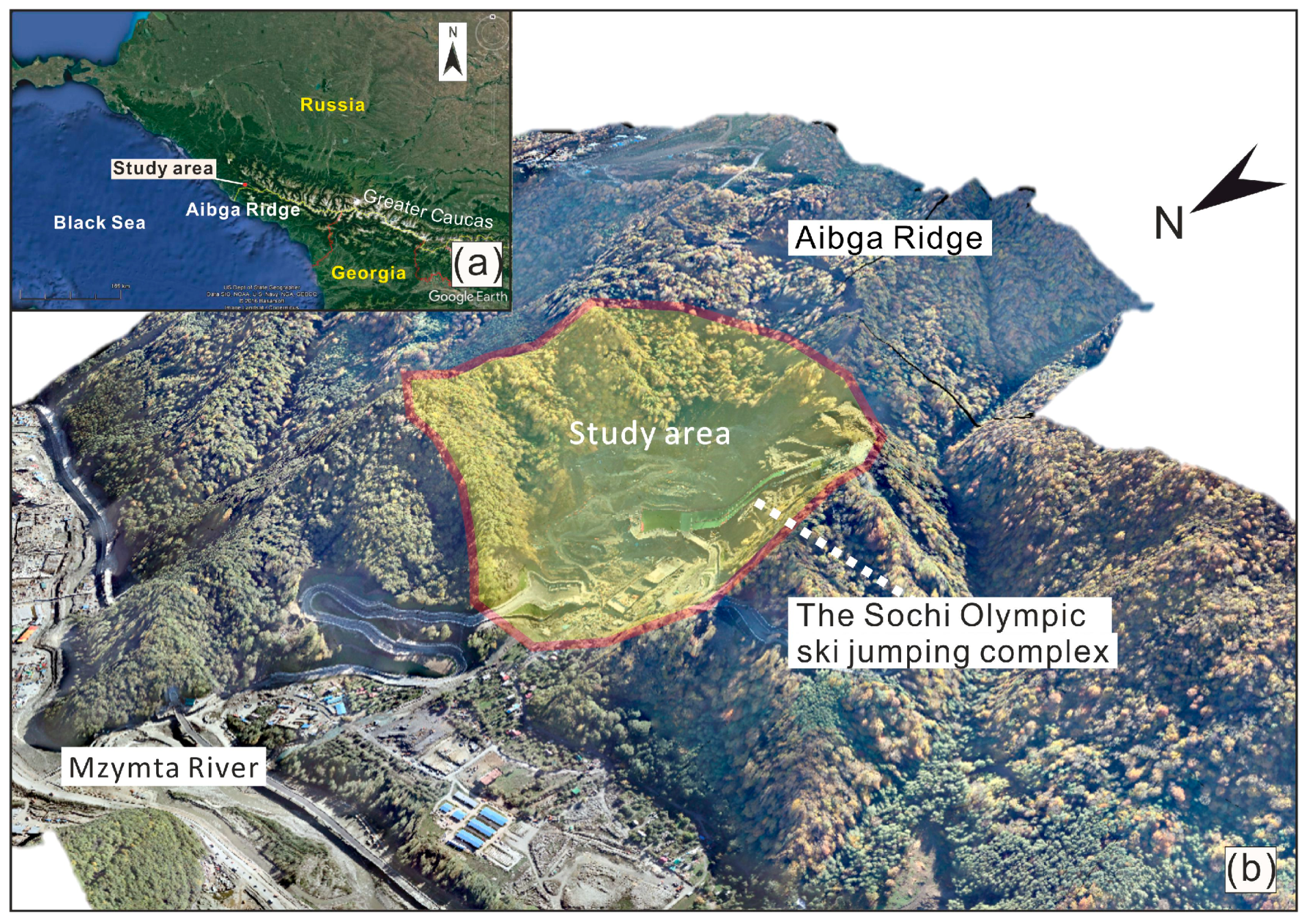
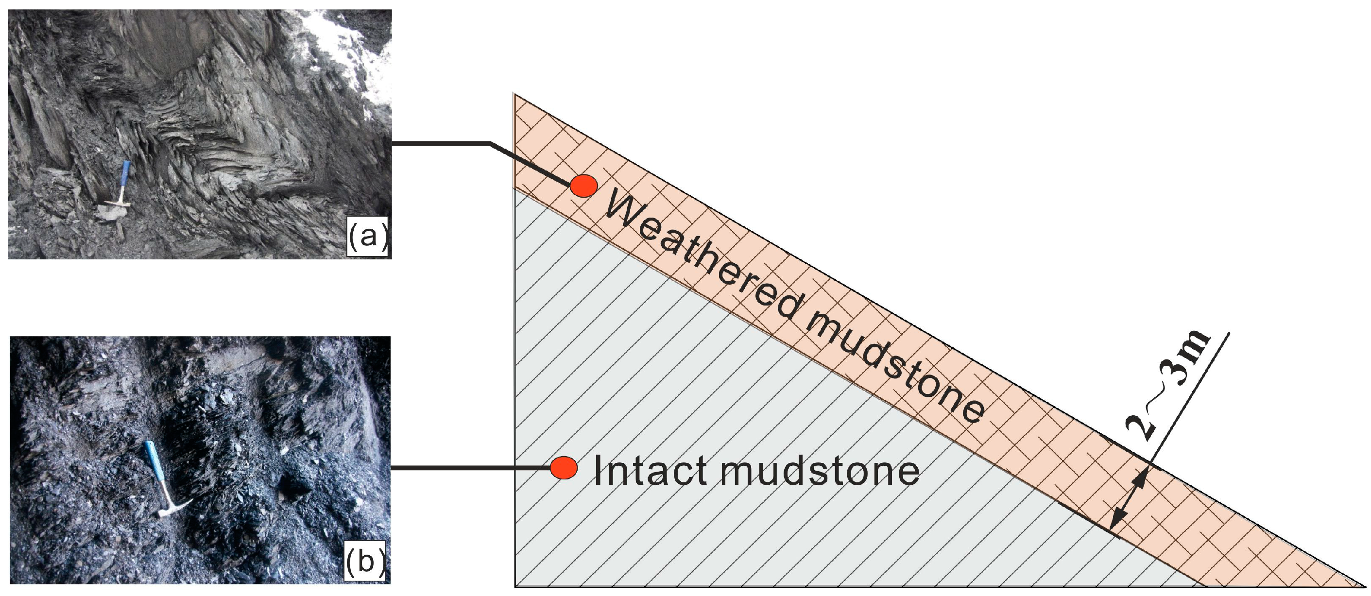
2.1. General Geographical and Geological Background

The Olympic ski-jump complex in Sochi, Russia was selected as the study area. The area is located in the northern Caucasus on the east Black Sea coast (Figure 1a). The area is on the left bank of the Mzymta River and it covers an area of 0.53 km² (Figure 1b).

In recent years, some construction related to tourism has been planned. Some work has been carried out, so that the topography relief and the geological deposits have been changed. Some loss Quaternary deposits like sand and clay have been cleared out. Regarding geological conditions (Figure 2), most of the area is covered by Jurassic mudstone as outcropping bedrock. The upper layer of mudstone bedrock is widespread weathered mudstone. The intact mudstone of bedrock is of low permeability (0.001 m/d), while the weathered layer is more permeable (1 m/d). The thickness of the weathered mudstone all over the area is about 2–3 m. Due to the low strength of weathered layer, the area is supposed to be prone to landslide. Through the field investigation, some shallow landslide warning signs, such as new cracks and unusual bulges, could be found as shown in Figure 3. In this study, an earthquake is believed to be the primary trigger factor of landslide in Sochi ski-jump area, rather than rainfall. Therefore, rainfall-induced landslide has not been considered yet.

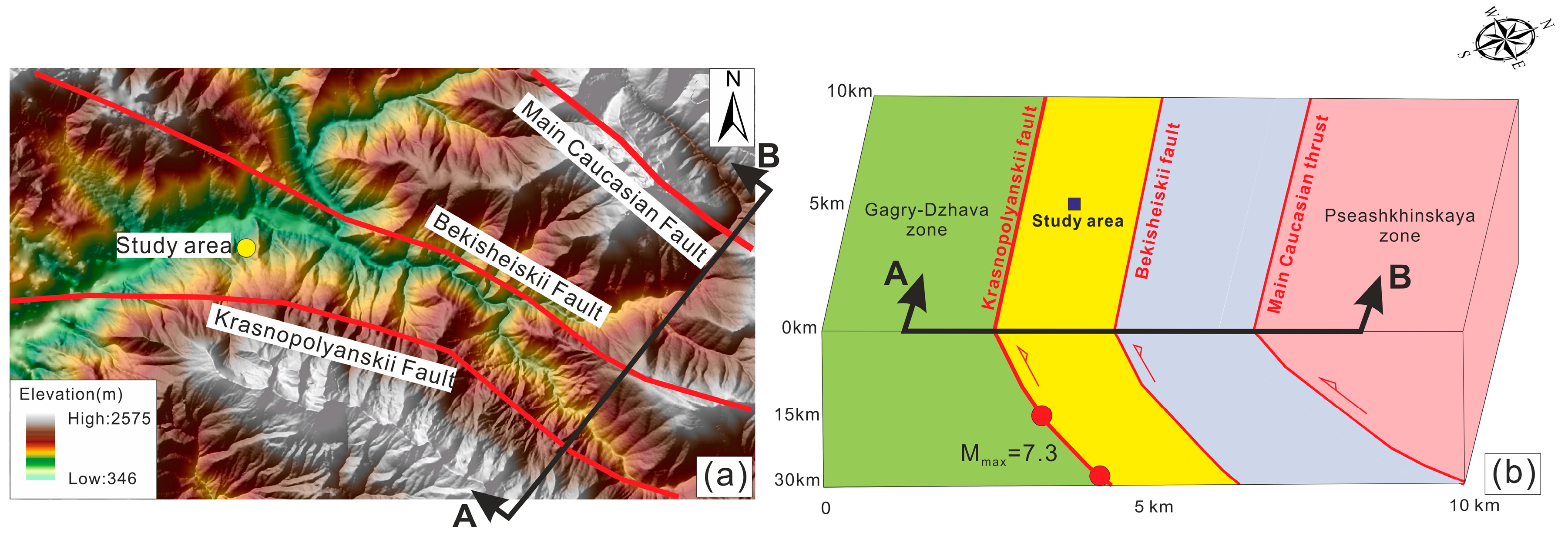
2.2. Geotectonic and Seismic Conditions of the Region

In terms of seismic hazard, the study area is of high seismic activity. According to the existing map of general seismic zoning (GSZ) of the Russian Federation (OSR-97), the territory of Sochi falls in the zone prone to seismic intensity of 8–9 [29]. The last strong earthquake, which triggered widespread distributed landslides, was thought to occur about 600 years ago [35]. The active faults of the Sochi region include Main Caucasian, Bekisheiskii, Krasnopolyanskii, Monastyrskii and Sochinskii faults [30]. All these active faults are reverse faults, except that the Main Caucasian is a thrust fault. According to the empirical relationship between the earthquake magnitude and the displacement on the fault, the fault displacement with an amplitude of 1.2 m corresponds to the magnitude Mw = 7.3, which is the maximum magnitude of the Sochi region [35].

As for the ski-jump area, the potential earthquake may be sourced from the Main Caucasian fault zone, Bekisheiskii fault zone, and Krasnopolyanskii fault zone (Figure 4a). These active faults in the study zone generally run from east-southwest to west-northeast and they run parallel to each other. As mentioned above, the Main Caucasian fault is a thrust fault; the Bekisheiskii and Krasnopolyanskii faults are reverse faults. In this paper, we consider the Krasnopolyanskii fault as the source of the potential earthquakes, which may represent the most negative seismic condition (Figure 4b).

As for the Caucasus region, the empirical relation of intensity (I_m) to magnitude (M) and hypocentral distance (D) and the empirical relation of peak ground acceleration (PGA) to intensity (I_m) are shown as follows [14]:

I_m = 1.5M − 4.7 lgD + 4.0,

(1)

lgPGA = 0.301 I_m − 3.1,

(2)

where I_m is the MSK-64 intensity, M is magnitude, D is distance between the hypocenter and the object location in kms, and PGA is the maximum horizontal acceleration in gs.

Note that D may respond to the hypocentral depth when the object is in the fault zone. In this study, the area was assumed located upon the earthquake source, as shown in Figure 4b. the distance D between the epicenter and the object location refers to the depth of the hypocenter. The depth of the hypocenter is assumed to range from 15 km to 30 km. According to the Equations (1) and (2), the assumed I_m and PGA of the study area were summarized, as shown in

Table 1. The seismic parameters related to maximum magnitude in study area.

Magnitude, M	Earthquake Hypocentral Depth, D (km)	MSK-64 Intensity, Im	Peak Ground Horizontal Acceleratio, PGA (g)	Horizontal Seismic Coefficient, Kh	Vertical Seismic Coefficient, Kv
7.3	15	9.4	0.44	0.22	0.07
7.3	20	8.8	0.30	0.15	0.05
7.3	25	8.4	0.20	0.1	0.033
7.3	30	8.0	0.16	0.08	0.026

.

The study aims to analyze shallow landslide susceptibility of the area under different seismic conditions. As the previous text shows, the conditions include earthquakes with hypocenters of different depth.

3. Data and Methods

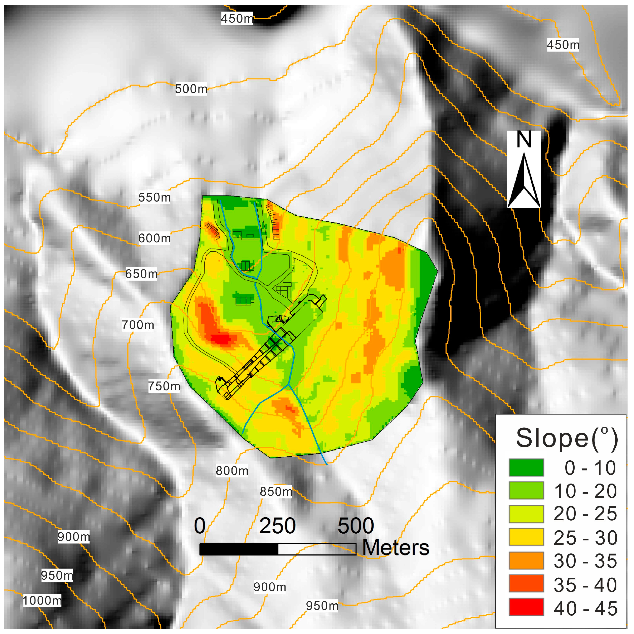
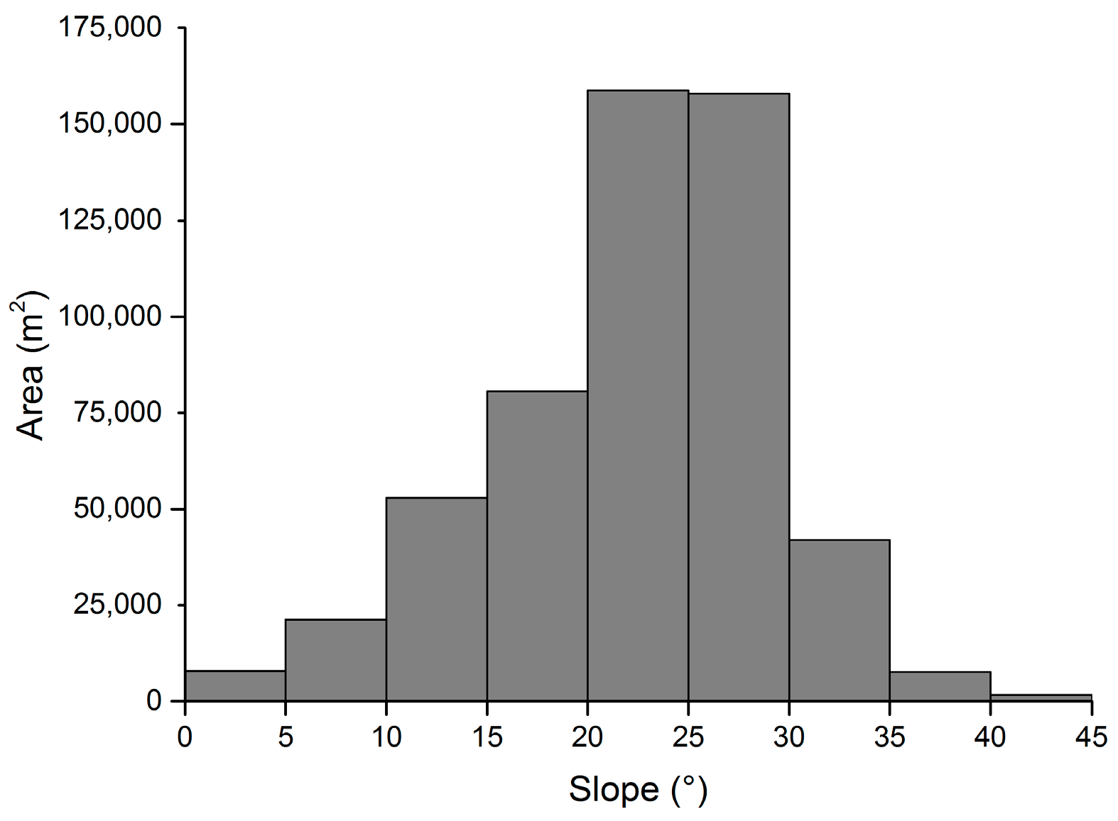
3.1. Topographic Data and Slope Map

A 5-m digital elevation model (DEM) with the 0.5-m error obtained from the aerial scanning data was used for topographic analysis. Topographic features were presented in ArcGIS (Figure 5). The slope map was created by using a simple algorithm from the DEM that compares the elevations of adjacent cells and calculates the maximum slope. Figure 5 showed the slopes with large slope angles (>40°), including two northern artificial scarps. The following analysis aims to assess natural slope susceptibility; therefore, the stability results of the northern artificial slopes will be excluded. According to the slope distribution map, the statistics of the study area with different slope angles were analyzed, as shown in Figure 6. The slope-angle analysis showed that the steepest slope is about 45° and the most distributed slope is between 20–30°. Therefore, the variation of the slope angles was achieved, which can be applied to classify the slope angle of slope models.

3.2. Slope Stability Numerical Modelling

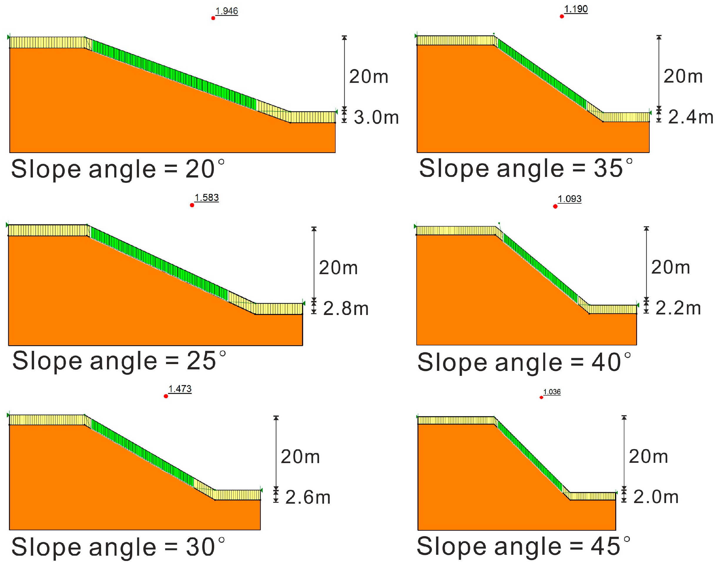
3.2.1. Slope Models

According to slope-angle distribution (Figure 6), six simplified mudstone slope models were set up in the GeoStudio software, as shown in Figure 7. The slope angles of models were set to be 20°, 25°, 30°, 35°, 40°, and 45°. The slope instability of the slope angle below 20° was not considered due to the results of initial calculation, in which the Fs of the slope of slope angle below 20° is hardly below 1.0 even in the most negative seismic condition. The slope model height was 20 m; the thickness of weathered mudstone was 2–3 m. Through the field investigation, the steepest slopes have the minimum thickness of weathered mudstone, while the thickness of weathered mudstone in the slope with a slope angle 20° is about 3 m. Therefore, the thickness of weathered mudstone in 45° slope was set to be 2 m, and the weathered layer thickness in 20° slope −3 m. The weathered mudstone thickness value in other slope models (with slope angle 25°, 30°, 35°, 40°) was assigned by linear interpolation. In addition, the tension cracks were set in the weathered mudstone. These models aim to analyze the shallow slope instability.

3.2.2. Physical–Mechanical Parameters of Mudstone

Based on the experimental result, the typical physical–mechanical parameters of weathered mudstone are taken as follows: the unit weight is 19 kN/m³, cohesion is 10 kPa and friction angle is 27°. As for intact mudstone, the unit weight is taken to be 22 kN/m³, cohesion-25 kPa and friction angle is 28°. Note that the intact mudstone refers to the lower layer close to the weathered mudstone. The above parameters were, then, used as input in numerical calculation of slope stability analysis.

3.2.3. Spencer Method of Slope Stability Analysis

The limit equilibrium method for analysis of slope stability has been applied in geotechnical engineering for many decades. According to the method, the landslide body is divided into many slices in order to analyze mechanical state. The main concept of limit equilibrium method is to get safety factor with respect to horizontal force equilibrium equation or moment equilibrium equation. The safety factor is calculated by comparing the resistance with the sliding strength of the slope. When the safety factor is above 1.0, the slope is supposed to be stable. When the safety factor is below 1.0, the slope is believed to be unstable. The slope is more stable as the safety factor is bigger.

The safety factor equation with respect to force equilibrium is:

$${\mathrm{F}}_{\mathrm{s}-\mathrm{f}}=\frac{{\displaystyle \sum (N_i\tan {\varphi }_i\cos \alpha +c_i{l}_i\cos \alpha })}{{\displaystyle \sum N_i\sin \alpha }},$$

(3)

where c_i is cohesion of i-th slice, φ_i is friction angle of i-th slice, α is inclination of slice base, N_i is slice base normal force and l_i is geometric parameter.

The safety factor equation with respect to moment equilibrium is:

$${\mathrm{F}}_{\mathrm{s}-\mathrm{m}}=\frac{({\displaystyle \sum N_i\tan {\varphi }_i+{\displaystyle \sum c_i{l}_i}})R}{{\displaystyle \sum G_{i}x-{\displaystyle \sum N_{i}f}}},$$

(4)

where G_i is i-th slice weight; R, x and f are geometric parameters; others are the same as Equation (3).

Spencer developed a method accessing safety factor satisfying both force and moment equilibrium [28]. In the Spencer method, interslice shear to normal ratio is a constant, which makes the two safety factors from Equations (3) and (4) equal. As a type of limit equilibrium method, the Spencer method has mathematically more rigorous formulations rather than traditional methods like the Janbu method [36] and Bishop [37] method. The detailed content can be referred to Spencer’s study [28]. In a word, the safety factor can be achieved through the Spencer method based on the material unit weight, cohesion, friction angle, and slope angle (the slope model geometry).

3.2.4. Pseudostatic Analysis

The pseudostatic analysis shows the seismic effects by an earthquake’s ground accelerations that leads to inertial forces. The direction of seismic forces can be horizontal and vertical at the centroid of each slice while using the Spencer method (Figure 8). The horizontal and vertical seismic forces are defined as:

$$F_h=\frac{a_h}{g}G=K_{h}G,$$

(5)

$$F_v=\frac{a_v}{g}G=K_{v}G,$$

(6)

where a_h and a_v are horizontal and vertical pseudostatic accelerations, g is the gravitational acceleration constant, G is slice weight, K_h and K_v are horizontal and vertical seismic coefficients.

In this study, the selection of seismic coefficients was based on Eurocode 8 [38]: a_h is considered as half of PGA, while, a_v is equal to 0.33 a_h. Therefore, K_h and K_v can be computed on the basis of PGA values responding to different earthquake conditions, as shown in Table 1.

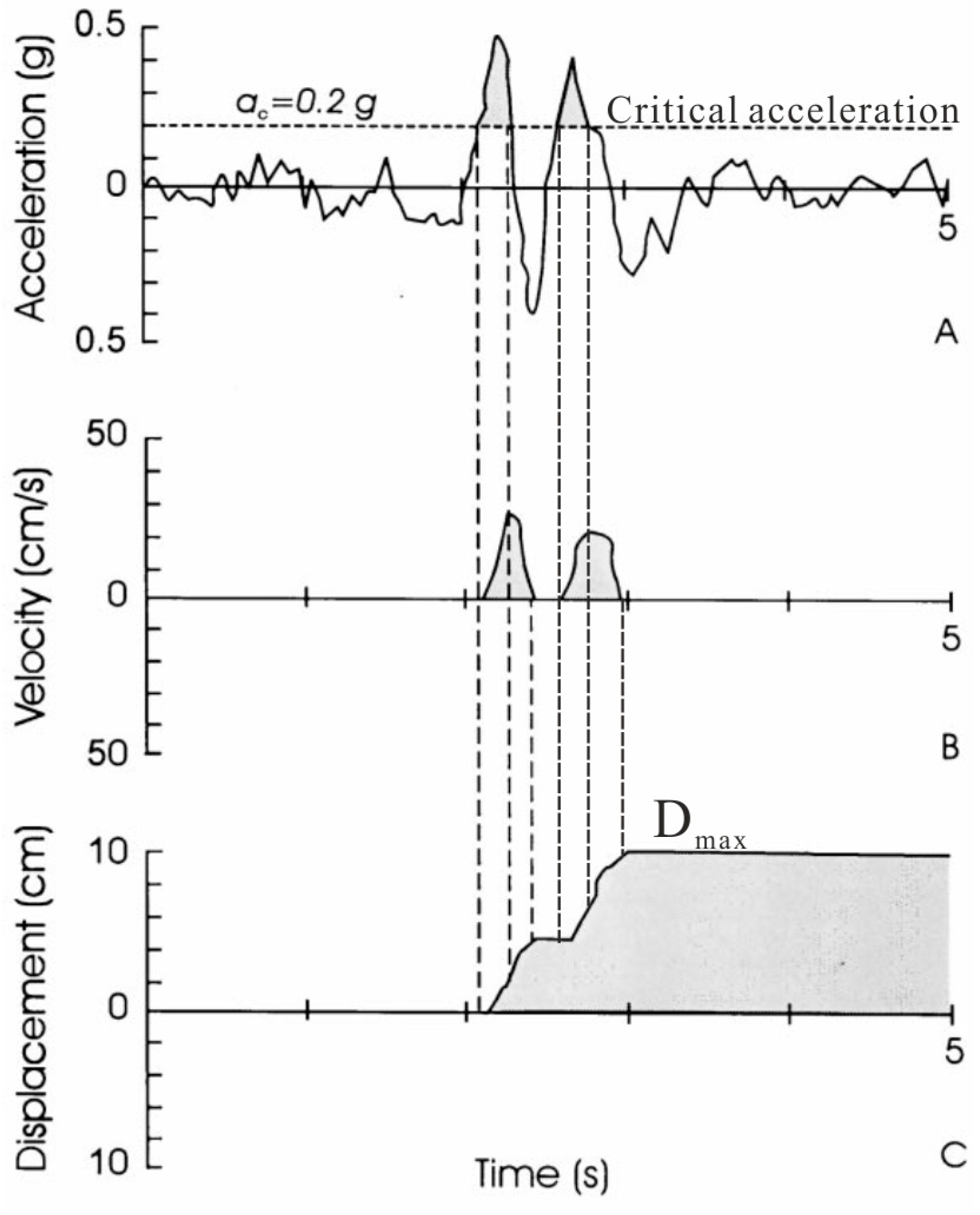
3.2.5. Newmark Deformation Method

In 1965, Newmark introduced a method of analysis for estimating deformations of an artificial embankment dam owing to strong shaking caused by an earthquake [31]. This method was called the Newmark method and then used in natural slope analysis. At present, the Newmark method is usually applied to evaluate the performance of landslides induced by an earthquake. The main concept is to estimate accumulated displacement of the slope through doubly integrating the acceleration over the critical acceleration in the sliding block, as shown in Figure 9.

The sliding block has a critical acceleration, a_c, which represents the threshold to overcome resistance to starting to slide. Newmark pointed out that the critical acceleration is a function of the static safety factor and slope angle, defined as:

a_c = (Fs − 1)·g sinα,

(7)

where a_c is the critical acceleration, g is gravity acceleration, Fs is the static safety factor, and α is slope angle.

To get Newmark displacement requires knowing the static safety factor, the slope angle and selecting an earthquake ground strong-motion record. After considering a large number of strong-motion records, Jibson and et al. developed an empirical regression equation to estimate Newmark displacement [16]. The regression equation of Newmark displacement is a function of critical acceleration and Arias intensity, expressed as:

lg D_n = 1.521 lg I_a − 1.993 lg a_c − 1.546,

(8)

where D_n is Newmark displacement in centimeters, I_a is the Arias intensity in meters per second, and a_c is the critical acceleration in gs.

Since Russia adopts MSK-64 intensity, the regression equation of Newmark displacement requires to be a function of critical acceleration and MSK-64 intensity. Based on the study of Margottini et al. [39], Arias intensity can be transformed into MSK-64 intensity through an equation as follows:

lg I_a = −1.079 + 0.31 I_m,

(9)

where I_a is the Arias intensity, I_m is the MSK-64 intensity.

Combining Equations (8) and (9), we can get the regression equation of Newmark displacement as a function of critical acceleration and MSK-64 intensity:

lg D_n = 0.162 I_m − 1.993 log a_c − 3.187,

(10)

As mentioned in the previous context, four different seismic conditions are considered with respect to magnitude 7.3 and earthquake hypocentral depth 15–30 km. The MSK-64 intensity can be calculated by Equation (1), as shown in Table 1. Once intensity is known, Newmark displacements D_n in these conditions can be expressed as follows,

As for earthquake hypocentral depth 15 km:

lg D_n = −1.993 log a_c − 1.67,

(11)

As for earthquake hypocentral depth 20 km:

lg D_n = −1.993 log a_c − 1.76,

(12)

As for earthquake hypocentral depth 25 km:

lg D_n = −1.993 log a_c − 1.83,

(13)

As for earthquake hypocentral depth 30 km:

lg D_n = −1.993 log a_c − 1.89,

(14)

4. Results

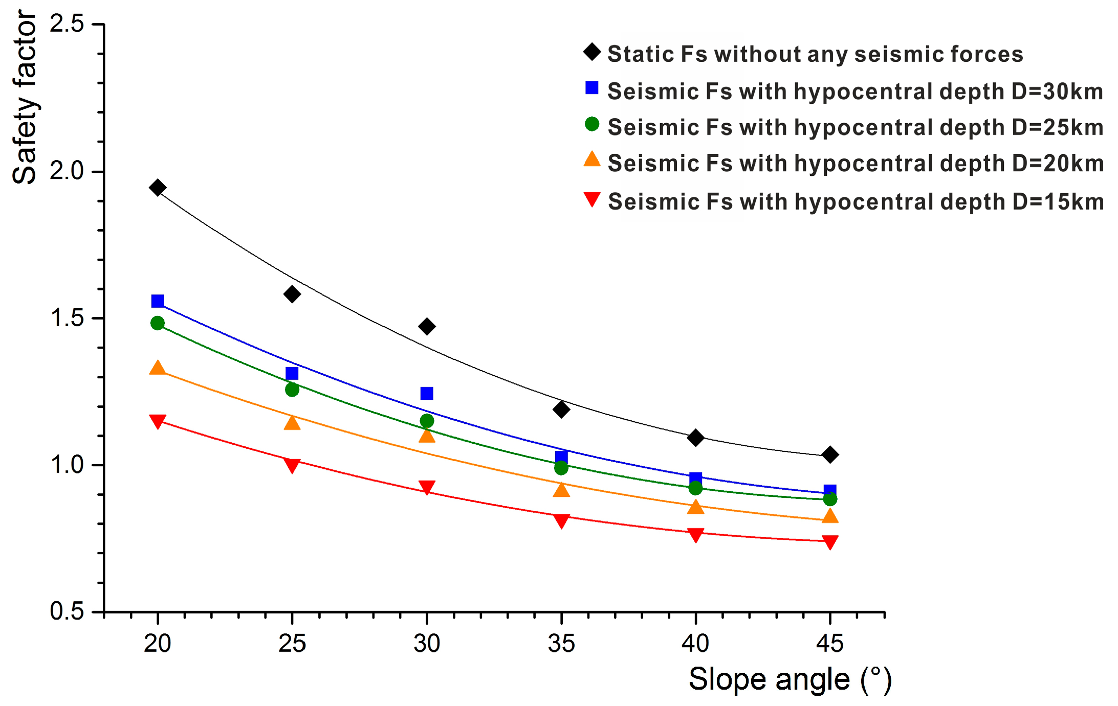
4.1. Relationships of Safety Factor to Slope Angle

The variation of physical–mechanical parameters may influence the results of Fs. However, the variation of parameters is limited for the study area. Therefore, the mean values were selected to use in numerical modelling. As the physical-mechanical parameters were fixed, the relationship of safety factor to slope angle was specifically analyzed.

Numerical modelling was conducted for slope models from 6 different slope angles (20°, 25°, 30°, 35°, 40°, and 45°), as shown in Figure 7. Static and seismic safety factors were computed using Spencer method. Applying pseudostatic analysis, seismic slope stability modelling included 4 conditions, in which seismic coefficients F_h and F_v were used, referring to Table 1.

The results of safety factor in either static or seismic states, plotted in Figure 10, turned out to fit polynomial curves. It could be found that the regression equations were well constrained (R² > 0.96). The resulting regression equations between the safety factor and slope angle are expressed as shown in

Table 2. The relationships of safety factor to slope angle in deferent conditions.

Condition of Numerical Modelling	Magnitude, M	Earthquake Hypocentral Depth, D (km)	Regression Equations between Safety Factor (Fs) and Slope Angle (α)
Static	None	-	Fs = 0.0011α2 − 0.110α + 3.6686; R2 = 0.984 *
Seismic	7.3	15	Fs = 0.0005α2 − 0.051α + 1.9516; R2 = 0.993
Seismic	7.3	20	Fs = 0.0005α2 − 0.054α + 2.1955; R2 = 0.975
Seismic	7.3	25	Fs = 0.0008α2 − 0.075α + 2.6613; R2 = 0.994
Seismic	7.3	30	Fs = 0.0007α2 − 0.073α + 2.7166; R2 = 0.980

* R² means a coefficient of determination of the regression equation.

.

Since the slope map was made, the relationship of the safety factor to slope angle helped to conduct safety factor maps. Then, the equations were implemented based on the ArcGIS program in order to produce safety factor maps.

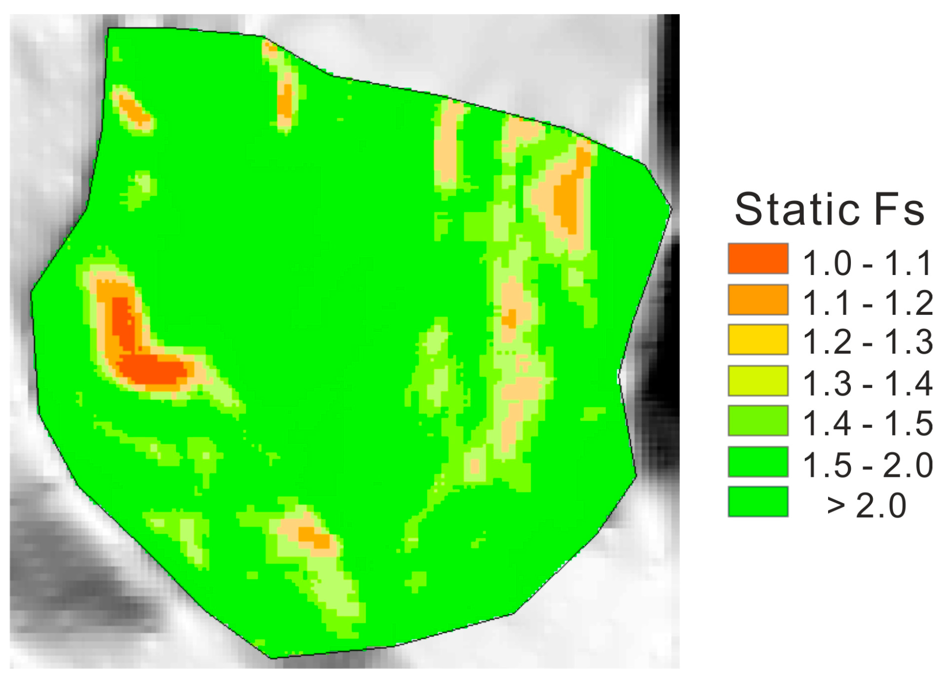
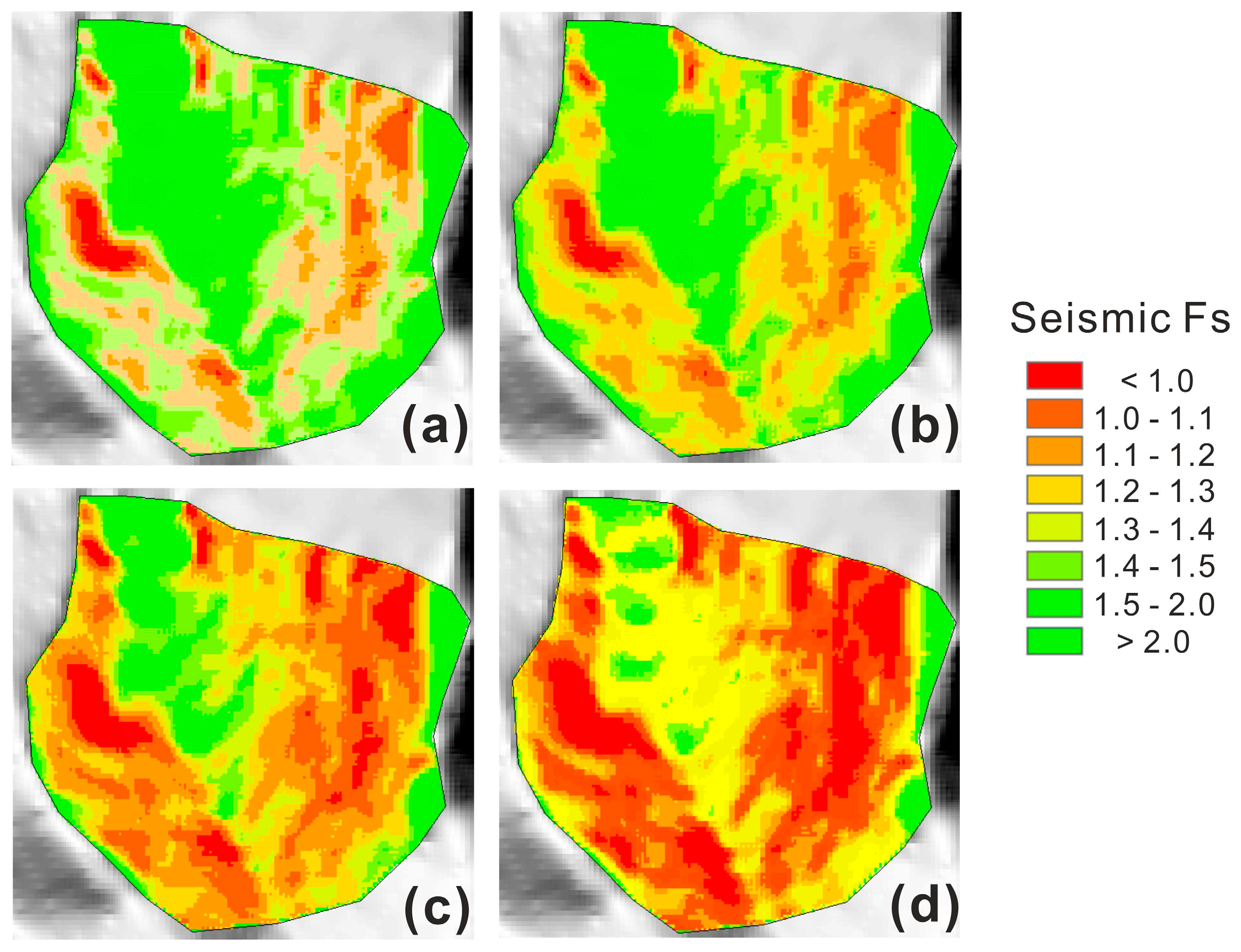
4.2. Static and Seismic Safety Factor Mapping

Since the slope map (Figure 5) derived from DEM has been achieved, the safety factor maps can be drawn based on the regression equations between the safety factor and slope angle. The mapping process was carried out using the raster calculation tool in ArcGIS program.

Figure 11 shows the static safety factor map. From the figure, we could see the western part of the area suffered the lowest safety factors, the value of which is near 1.0. As mentioned above, slope stability or instability is based on the interplay between driving forces and resisting forces: when driving forces overcome resisting forces (Fs < 1.0), the slope is unstable and it results in slope failure. According to the field investigation, the slopes possessing the lowest safety factors turned out to be the most vulnerable to slope failure, with landslide warning signs investigated. Because the safety factor is above 1.0, the entire slope failure has not occurred yet. Compared with the landslide warning sign locations in Figure 3, the static safety factor map of Figure 11 corresponds to the actual potential landslide map, which could verify the model validation.

The seismic safety factor maps were drawn with respect to hypocentral depth 30 km (Figure 12a), hypocentral depth 25 km (Figure 12b), hypocentral depth 20 km (Figure 12c), and hypocentral depth 15 km (Figure 12d). Results of seismic safety factor maps indicate that the area of Fs below 1.0 expands, as hypocentral depth decreases: when hypocentral depth is 30 km, the slope instability occurs only in small parts of western and eastern slopes; when hypocentral depth is 15 km, the slope failure appears all over the area except for northern and central area.

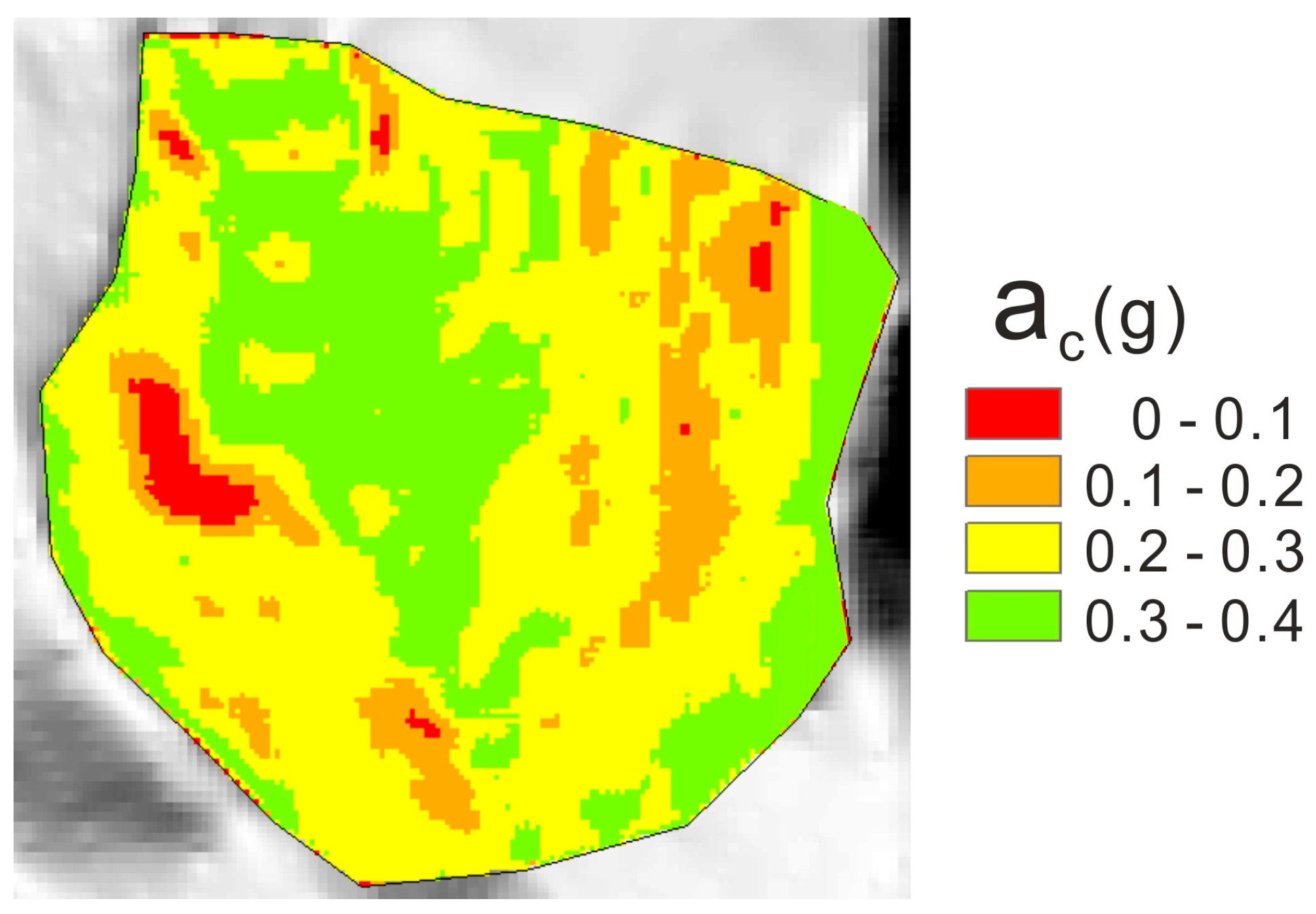
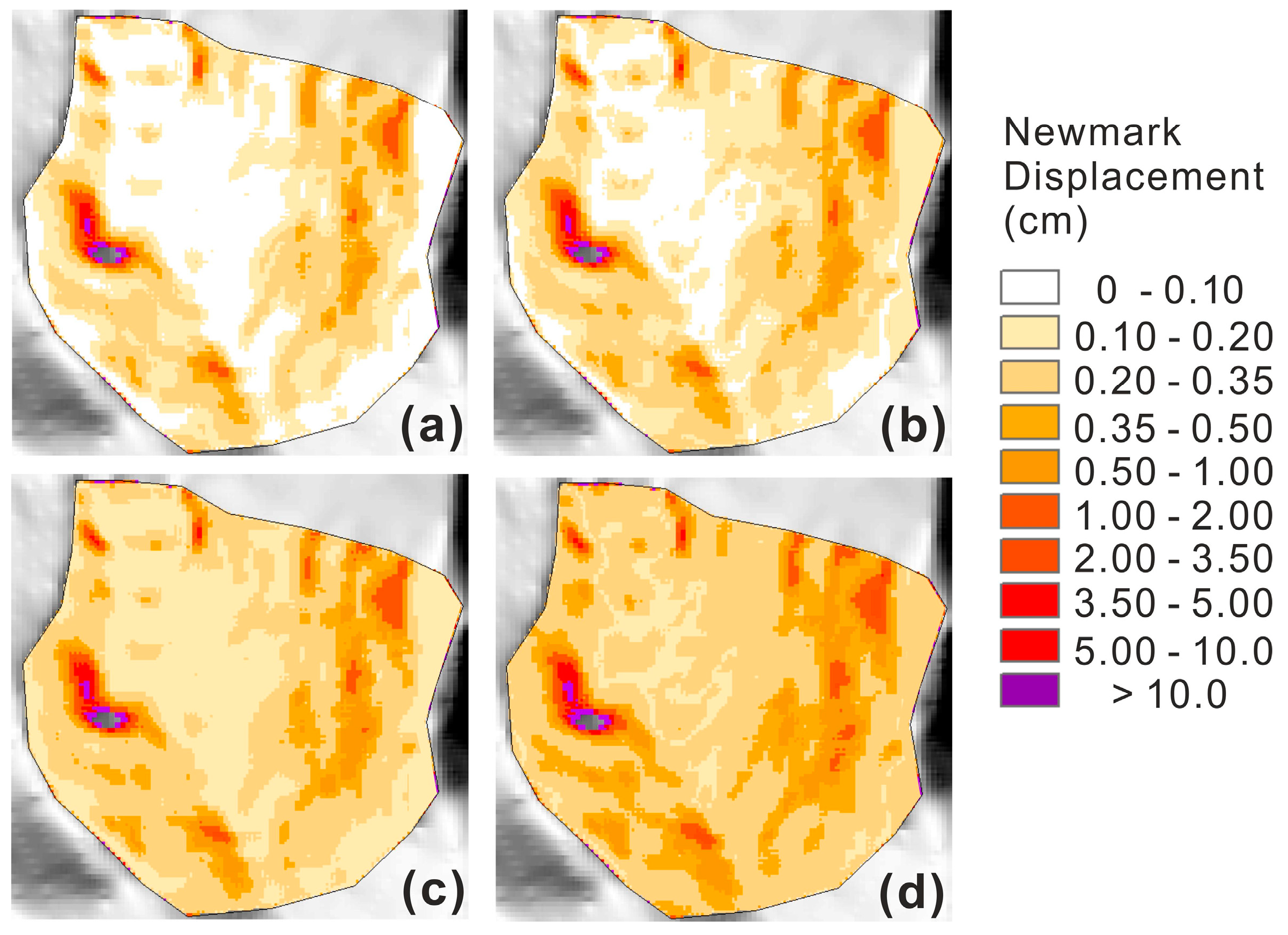
4.3. Newmark Deformation Mapping

As indicated above, conducting a Newmark displacement map requires the critical acceleration map according to Equations (1)–(4). First, the critical acceleration map was made, based on a function of the static safety factor and slope angle, the values of which had been known. The critical acceleration map is shown in Figure 13. Finally, the predicted Newmark displacements under potential earthquakes were estimated in each raster cell, which made up the Newmark displacement map (Figure 14). From the Newmark displacement maps, we can see that the largest displacement (>10 cm) occurs in the western slopes, correlated with the part of the lowest safety factors. The result also indicates that Newmark displacement increases, as the hypocentral depth decreases. Under condition of earthquake with hypocentral depth of 15 km, the entire area suffers the ground movement, however, most parts of the area will move less than 0.35 cm. The most dangerous slopes, which may undergo the largest displacement, are believed to be the western part of the area.

5. Discussion and Conclusions

The method combining GIS and numerical modelling were proposed. After numerical calculation of 6 slope models with different slope angles, the relationships between safety factor and slope angle were acquired. From the relationships of safety factor to slope angle, it can be concluded that safety factor decreases as slope angle increases. Also, safety factor is proved to decrease as seismic effect (K_c) increases. The results are easy to understand, however, we found that under either static or seismic conditions the relationships of safety factor to slope angle can be fitted by polynomial curves. Using the regression equations, it was easier to conduct safety factor maps in GIS.

According to the static safety factor map, the western slopes of the area were believed to be the most vulnerable to slope failure. The result of the lowest Fs in the static safety factor map is correlated with field performance, where the landslide warning signs occurred. As the hypocentral depth decreases, the seismic effect increases. The seismic safety factor maps give an approach to investigate the safety factor variation due to the change of seismic effect.

The transformed Newmark-displacement equations based on MSK-64 intensity were presented. The result shows that the Newmark displacement is supposed to increase, as the seismic effect increases. In addition, the slopes with the largest Newmark displacements correspond to the ones with the lowest safety factors. Newmark displacement maps provide an index to predict the landslide susceptibility.

The shortcomings of this study are lack of comparison of the predicted Newmark displacement with the actual landslide performance. This is due to the fact that the study area has been rebuilt and the last earthquake inducing the widespread landslides in this region occurred 600 years ago. Future work will expand the scope of the study area, considering the inventory of landslides triggered by historical earthquakes.

References

1. Nadim, F.; Kjekstad, O.; Peduzzi, P.; Herold, C.; Jaedicke, C. Global landslide and avalanche hotspots. Landslides 2006, 3, 159–173. [Google Scholar] [CrossRef]
2. Fedorovsky, V.G.; Kurillo, S.V.; Kryuchkov, S.A.; Bobyr, G.A.; Dzhantimirov, K.A.; Iliyn, S.V.I.; Iliyn, S.; Kharlamov, P.V.; Rytov, S.A.; Skorokhodov, A.G.; et al. Geotechnical Aspects of Design and Construction of the Mountain Cluster Olympic Facilities in Sochi. In Proceedings of the 18th International Conference on Soil Mechanics and Geotechnical Engineering, Paris, France, 2–6 September 2013; pp. 3099–3102. [Google Scholar]
3. Ponomarev, A.A.; Zerkal, O.V.; Samarin, E.N. Protection of the transport infrastructure from influence of landslides by suspension grouting. Procedia Eng. 2017, 189, 880–885. [Google Scholar] [CrossRef]
4. Huang, S.; Wang, J.; Qiu, Z.; Kang, K. Effects of Cyclic Wetting-Drying Conditions on Elastic Modulus and Compressive Strength of Sandstone and Mudstone. Processes 2018, 6, 234. [Google Scholar] [CrossRef]
5. Corominas, J.; Martínez-Bofill, J.; Soler, A. A textural classification of argillaceous rocks and their durability. Landslides 2014, 12, 669–687. [Google Scholar] [CrossRef]
6. Zerkal, O.V.; Kalinin, E.V.; Panasyan, L.L. The Formation and Distribution of Stress Concentration Zones in Heterogeneous Rock Masses with Slopes. In Proceedings of the XII International IAEG Congress on Engineering Geology for Society and Territory; Springer: New York, NY, USA, 2015; Volume 2, pp. 1251–1254. [Google Scholar] [CrossRef]
7. van Westen, C.J.; van Asch, T.W.J.; Soeters, R. Landslide hazard and risk zonation—Why is it still so difficult? Bull. Eng. Geol. Environ. 2005, 65, 167–184. [Google Scholar] [CrossRef]
8. Guzzetti, F.; Reichenbach, P.; Ardizzone, F.; Cardinali, M.; Galli, M. Estimating the quality of landslide susceptibility models. Geomorphology 2006, 81, 166–184. [Google Scholar] [CrossRef]
9. Dou, J.; Yamagishi, H.; Pourghasemi, H.R.; Yunus, A.P.; Song, X.; Xu, Y.; Zhu, Z. An integrated artificial neural network model for the landslide susceptibility assessment of Osado Island, Japan. Nat. Hazards 2015, 78, 1749–1776. [Google Scholar] [CrossRef]
10. Lin, L.; Lin, Q.G.; Wang, Y. Landslide susceptibility mapping on a global scale using the method of logistic regression. Nat. Hazard Earth Syst. 2017, 17, 1411–1424. [Google Scholar] [CrossRef]
11. Dou, J.; Yunus, A.P.; Tien Bui, D.; Merghadi, A.; Sahana, M.; Zhu, Z.; Chen, C.W.; Khosravi, K.; Yang, Y.; Pham, B.T. Assessment of advanced random forest and decision tree algorithms for modeling rainfall-induced landslide susceptibility in the Izu-Oshima Volcanic Island, Japan. Sci. Total Environ. 2019, 662, 332–346. [Google Scholar] [CrossRef]
12. Juliev, M.; Mergili, M.; Mondal, I.; Nurtaev, B.; Pulatov, A.; Hubl, J. Comparative analysis of statistical methods for landslide susceptibility mapping in the Bostanlik District, Uzbekistan. Sci. Total Environ. 2019, 653, 801–814. [Google Scholar] [CrossRef]
13. Qiu, C.; Esaki, T.; Xie, M.; Mitani, Y.; Wang, C. Spatio-temporal estimation of shallow landslide hazard triggered by rainfall using a three-dimensional model. Environ. Geol. 2006, 52, 1569–1579. [Google Scholar] [CrossRef]
14. Zakharov, V.S.; Simonov, D.A.; Koptev, A.V. Computational modelling of seismic landslide displacement. GEOprofile 2009, 1, 1–24. (In Russian) [Google Scholar]
15. Kuzin, A.A.; Grishchenkova, E.N.; Mustafin, M.G. Prediction of Natural and Technogenic Negative Processes Based on the Analysis of Relief and Geological Structure. Procedia Eng. 2017, 189, 744–751. [Google Scholar] [CrossRef]
16. Jibson, R.W.; Harp, E.L.; Michael, J.A. A method for producing digital probabilistic seismic landslide hazard maps. Eng. Geol. 2000, 58, 271–289. [Google Scholar] [CrossRef]
17. Ingles, J.; Darrozes, J.; Soula, J.C. Effects of the vertical component of ground shaking on earthquake-induced landslide displacements using generalized Newmark analysis. Eng. Geol. 2006, 86, 134–147. [Google Scholar] [CrossRef]
18. Chen, C.-W.; Chen, H.; Wei, L.-W.; Lin, G.-W.; Iida, T.; Yamada, R. Evaluating the susceptibility of landslide landforms in Japan using slope stability analysis: A case study of the 2016 Kumamoto earthquake. Landslides 2017, 14, 1793–1801. [Google Scholar] [CrossRef]
19. Krahn, J. Stability Modeling with SLOPE/W, An Engineering Methodology, 3rd ed.; GEO-SLOPE International Ltd.: Calgary, AB, Canada, 2007; p. 355. [Google Scholar]
20. Dawson, E.M.; Roth, W.H.; Drescher, A. Slope stability analysis by strength reduction. Geotechnique 1999, 49, 835–840. [Google Scholar] [CrossRef]
21. Griffiths, D.V.; Lane, P.A. Slope stability analysis by finite elements. Geotechnique 1999, 49, 387–403. [Google Scholar] [CrossRef]
22. Itasca Consulting Group Inc. FLAC3D (Fast Lagrangian Analysis of Continua in 3 Dimensions) User’s Manua (Version 5.0); Itasca Consulting Group Inc.: Minneapolis, MN, USA, 2012. [Google Scholar]
23. Tang, C.-L.; Hu, J.-C.; Lin, M.-L.; Angelier, J.; Lu, C.-Y.; Chan, Y.-C.; Chu, H.-T. The Tsaoling landslide triggered by the Chi-Chi earthquake, Taiwan: Insights from a discrete element simulation. Eng. Geol. 2009, 106, 1–19. [Google Scholar] [CrossRef]
24. Li, X.; He, S.; Luo, Y.; Wu, Y. Simulation of the sliding process of Donghekou landslide triggered by the Wenchuan earthquake using a distinct element method. Environ. Earth Sci. 2011, 65, 1049–1054. [Google Scholar] [CrossRef]
25. Bogomolov, A.N.; Matsiy, S.I.; Babakhanov, B.S.; Bezuglova, E.V.; Leyer, D.V.; Kuznetsova, S.V. Landslide stabilization on the section of the railroad construction in Sochi. Vestnik Volgograd. Gosudarstvennogo Arhitekturno-Stroitelnogo Univ. Stroitel. Arhitektura 2012, 29, 15–25. [Google Scholar]
26. Fomenko, I.K.; Zerkal, O.V. The Application of Anisotropy of Soil Properties in the Probabilistic Analysis of Landslides Activity. Procedia Eng. 2017, 189, 886–892. [Google Scholar] [CrossRef]
27. Kang, K.; Zerkal, O.V.; Huang, S.; Ponomarev, A.A. Roadway Slope Stability Assessment in Mudstone Layers of Sochi (Russia). In Geomechanics and Geodynamics of Rock Masses: Proceedings of EUROCK 2018, ISRM European Regional Symposium, Saint Petersburg, Russia; CRC Press: London, UK, 2018; Volume 2, pp. 1217–1222. [Google Scholar]
28. Spencer, E. A Method of Analysis of Embankments assuming Parallel Interslice Forces. Geotechnique 1967, 17, 11–26. [Google Scholar] [CrossRef]
29. Ulomov, V.I.; Shumilina, L.S. The Set of Maps of the General Seismic Risk Regionalization of the Territory of the Russian Federation, OSR-97. Scale 1:8000000, Explanatory Note and List of Cities and Populated Areas, Located in the Earthquake-Hazard Regions; Institute of Physics of the Earth RAS: Moscow, Russia, 2000; 57p. (In Russian) [Google Scholar]
30. Ovsyuchenko, A.N.; Khil’ko, A.V.; Shvarev, S.V.; Kostenko, K.A.; Marakhanov, A.V.; Rogozhin, E.A.; Novikov, S.S.; Lar’kov, A.S. Complex geological-geophysical study of active faults in the Sochi-Krasnaya Polyana region. Izvestiya Phys. Solid Earth 2013, 49, 859–881. [Google Scholar] [CrossRef]
31. Newmark, N.M. Effects of Earthquakes on Dams and Embankments. Geotechnique 1965, 15, 139–160. [Google Scholar] [CrossRef]
32. Wang, K.-L.; Lin, M.-L. Development of shallow seismic landslide potential map based on Newmark’s displacement: The case study of Chi-Chi earthquake, Taiwan. Environ. Earth Sci. 2009, 60, 775–785. [Google Scholar] [CrossRef]
33. Hsieh, S.-Y.; Lee, C.-T. Empirical estimation of the Newmark displacement from the Arias intensity and critical acceleration. Eng. Geol. 2011, 122, 34–42. [Google Scholar] [CrossRef]
34. Wang, Y.; Song, C.; Lin, Q.; Li, J. Occurrence probability assessment of earthquake-triggered landslides with Newmark displacement values and logistic regression: The Wenchuan earthquake, China. Geomorphology 2016, 258, 108–119. [Google Scholar] [CrossRef]
35. Rogozhin, E.A.; Ovsyuchenko, A.N.; Lutikov, A.I.; Sobisevich, A.L.; Sobisevich, L.E.; Gorbatikov, A.V. Endogenous Hazards of the Greater Caucasus; IFZ RAN: Moscow, Russia, 2014; 256p. (In Russian) [Google Scholar]
36. Janbu, N. Applications of Composite Slip Surfaces for Stability Analysis. In Proceedings of the European Conference on the Stability of Earth Slopes, Stockholm, Sweden, 20–25 September 1954; Volume 3, pp. 39–43. [Google Scholar]
37. Bishop, A.W.; Morgenstern, N. Stability coefficients for earth slopes. Geotechnique 1960, 10, 164–169. [Google Scholar] [CrossRef]
38. Comité Européen de Normalisation (CEN). Eurocode 8, Design of Structures for Earthquake Resistance—Part 5: Foundations, Retaining Structures and Geotechnical Aspects; European Standard NF EN 1998-5; CEN: Brussels, Belgium, 2004. [Google Scholar]
39. Margottini, C.; Molin, D.; Serva, L. Intensity Versus Ground Motion—A New Approach Using Italian Data. Eng Geol 1992, 33, 45–58. [Google Scholar] [CrossRef]
Figure 1. Location of the study area: (a) the area is located in northern Caucasus on the east Black Sea coast (based on Google Earth); (b) aerial scanning photo of the study area with the Sochi Olympic ski-jump facilities.
Ijgi 08 00148 g001
Figure 2. A typical slope profile of the study area. The main geological bedrock is Jurassic mudstone, including two layers: (a) the upper layer is weathered mudstone with thickness of around 2 m; (b) the lower layer is intact mudstone.
Ijgi 08 00148 g002
Figure 3. A slope instability map of the study area. The main existing landslide warning signs were found in the western part of the area; some also could be found in the southern and northeastern parts.
Ijgi 08 00148 g003
Figure 4. The tectonic schemes of the region: (a) the main active faults around the study area; (b) the schematic plot of the active faults with assumed earthquake focuses of different depth.
Ijgi 08 00148 g004
Figure 5. Slope map derived from the digital elevation model (DEM) of the study area (location shown in Figure 1). The steepest slope of 45° appears in the western part of the area. The two artificial scarps, also showing steep slopes, are located in the northern part of the area (see the legend of Figure 3).
Ijgi 08 00148 g005
Figure 6. The statistics concerning area distribution of different slope intervals: the steepest slope is about 45° and the most distributed slope is between 20–30°.
Ijgi 08 00148 g006
Figure 7. Slope models for stability analysis from 6 different slope angles (20°, 25°, 30°, 35°, 40°, and 45°) with static safety factors. The orange part responds to intact mudstone; the yellow part responds to weathered mudstone; the green part means the calculated landslide body.
Ijgi 08 00148 g007
Figure 8. Schematic map showing the directions of seismic forces in the slope slice in pseudostatic analysis. Note that for briefly presenting the seismic forces, the interslice forces and forces under the slice base are not shown in the stretch.
Ijgi 08 00148 g008
Figure 9. Schematic diagram indicating integration of acceleration to determine landslide block displacement (adapted from [16]). (A) Ground motion acceleration versus time with critical acceleration (horizontal dashed line). (B) Velocity of the sliding-block versus time. (C) Displacement of the sliding-block versus time.
Ijgi 08 00148 g009
Figure 10. Relationships between safety factor and slope angle with respect to static condition and four seismic conditions.
Ijgi 08 00148 g010
Figure 11. Static safety factor map of the study area (location shown in Figure 1).
Ijgi 08 00148 g011
Figure 12. Seismic safety factor maps of the study area (location shown in Figure 1), with respect to (a) hypocentral depth 30 km, (b) hypocentral depth 25 km, (c) hypocentral depth 20 km, and (d) hypocentral depth 15 km.
Ijgi 08 00148 g012
Figure 13. The critical acceleration map related to Newmark deformation calculation. The values represent the threshold of ground acceleration to overcome resistance for a landslide block to start to slide.
Ijgi 08 00148 g013
Figure 14. The predicted Newmark displacement maps: (a) in case of M 7.3 earthquake with hypocentral depth 30 km; (b) in the case of M 7.3 earthquake with hypocentral depth 25 km; (c) in case of M 7.3 earthquake with hypocentral depth 20 km; (d) in case of M 7.3 earthquake with hypocentral depth of 15 km.
Ijgi 08 00148 g014