Geographic Knowledge Graph (GeoKG): A Formalized Geographic Knowledge Representation

 ,
, 
 ,
,
Abstract
:1. Introduction
2. Related Works
2.1. Geographic Ontology
2.2. Geographic Knowledge Graph
3. Methodology
3.1. Basic Idea
3.1.1. Guiding Ideology
- Where is it? →space
- What is it like? →state
- Why is it there? →evolution
- When and how did it happen? →change
- What impacts does it have? →interaction
- How should it be managed for the mutual benefit of humanity and the natural environment? →usage
3.1.2. Main Elements
- Space →{object, location, time, relation, …}
- State →{object, time, location, attribute …}
- Evolution →{object, state, change, time, location, attribute, …}
- Change →{object, time, location, attribute, relation, …}
- Interaction →{object, relation, change, …}
- Usage →{object, change, state, …}
- Object-centered representation. All descriptions of the six aspects require geographic objects. Without objects, other elements are meaningless. Therefore, the six basic elements are formed around the object element.
- Combined representation. A description of a single basic element is just a statement. To represent these aspects in geography, the basic elements should be combined. Thus, all of the basic elements can be linked.
- Stepped representation. Note that the six aspects from the core geographical questions are not equal. Space and state focus on the static conditions of objects. Evolution and change pay more attentions to the dynamic conditions of objects. Moreover, interaction and usage rely on relationships and mechanisms between geographic objects. Thus, the basic elements cannot be treated as equals.
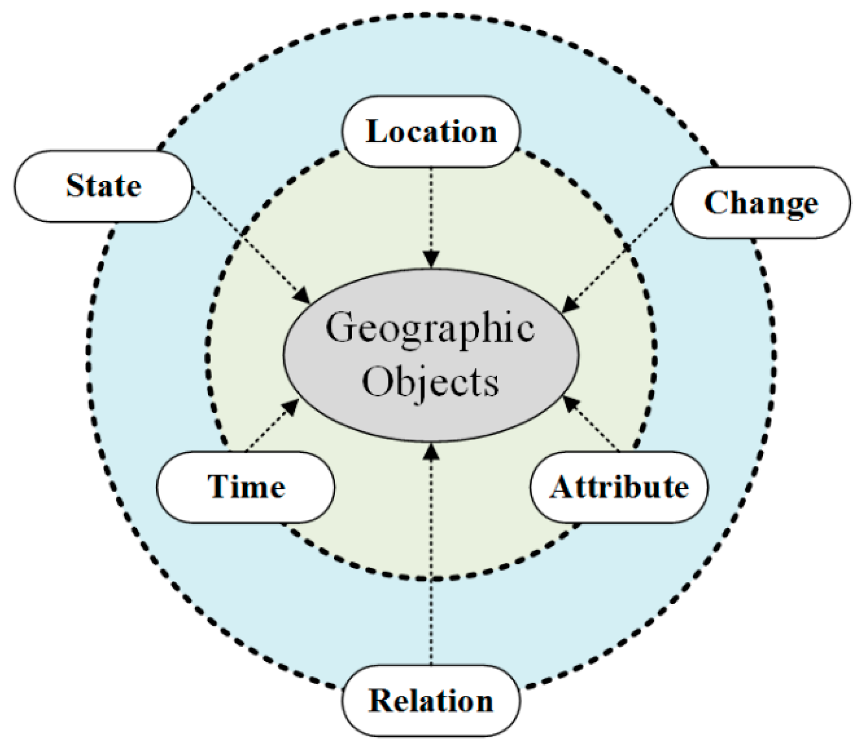
- A geographic object is the core of geographic knowledge representation and is the minimum unit to perceive the world. The six basic elements (location, time, attribute, state, change and relation) represent geographic knowledge from different perspectives, which are linked to geographic objects.
- Static independent geographic objects can be described by elements of location, time, and attribute. Location shows the spatial patterns of geographic objects. Time gives the temporal dimension of geographic objects for human cognition. Attribute describes the static features of geographic objects.
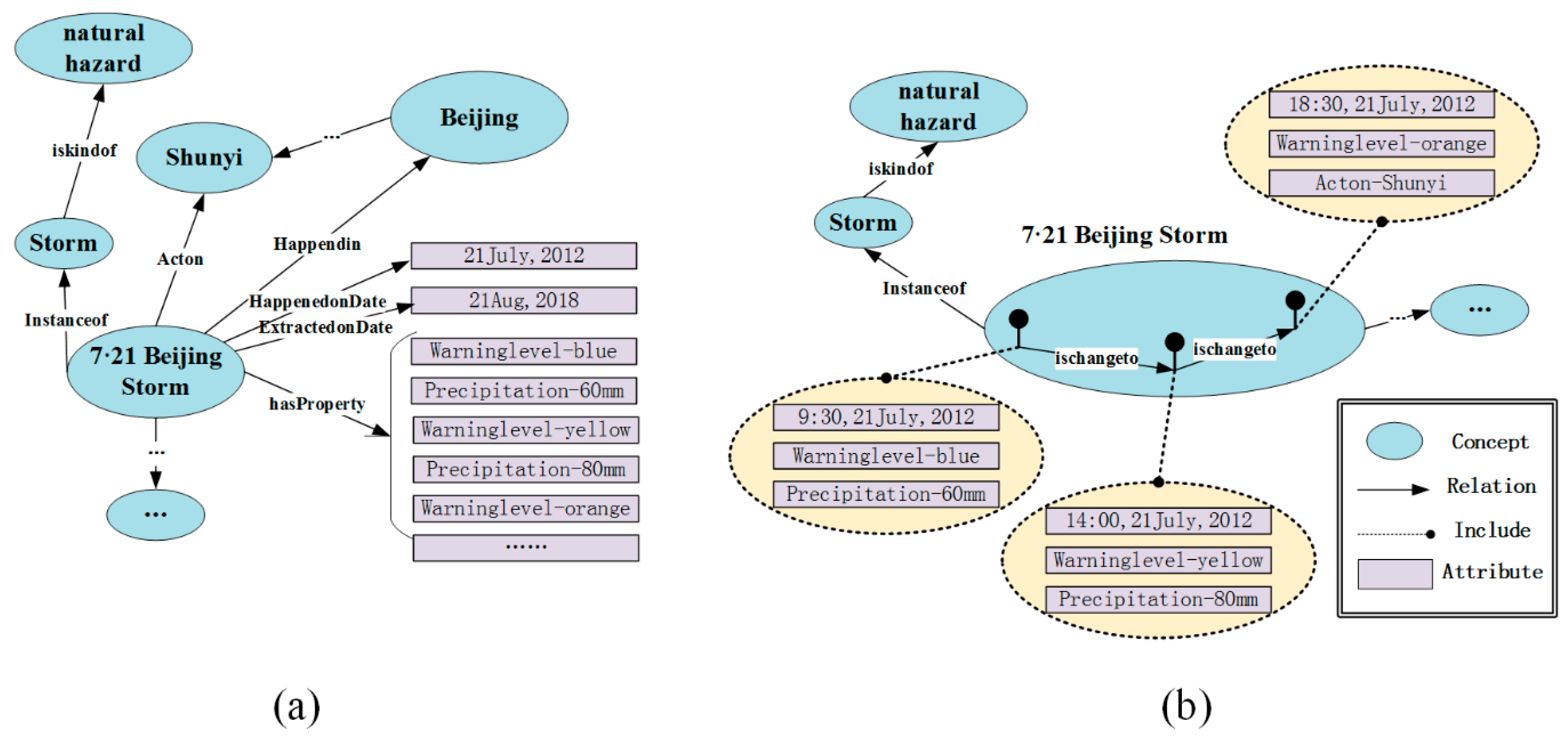
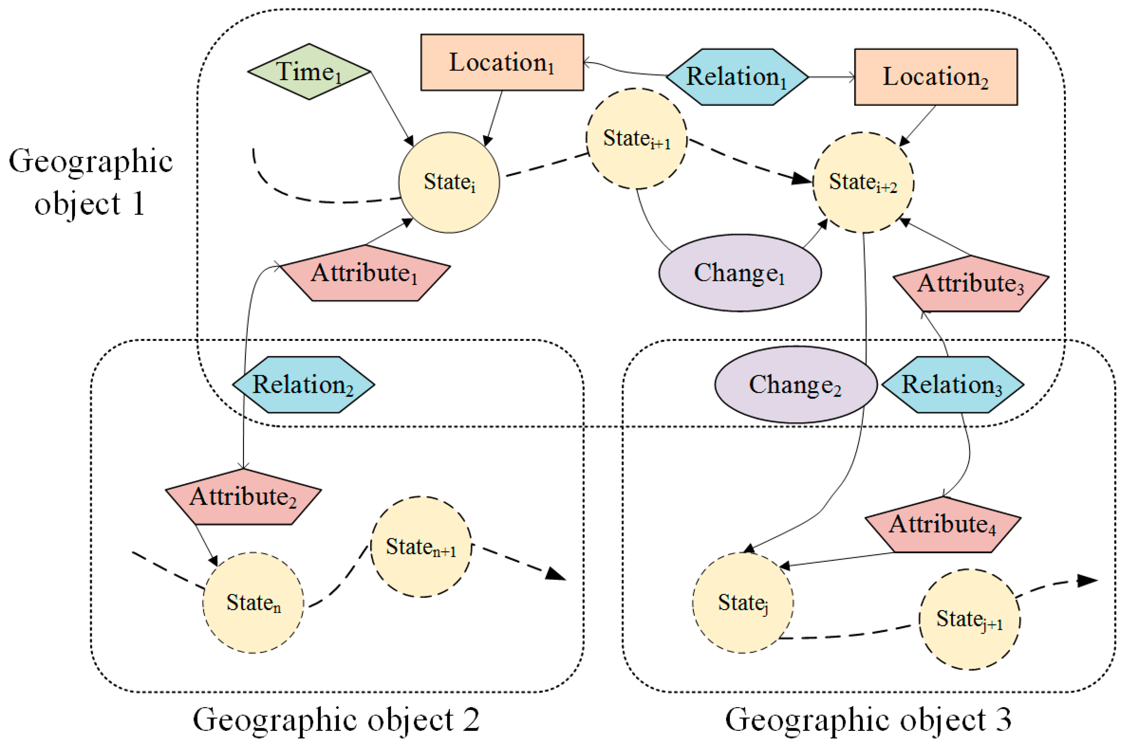
- Any geographic object has an entire life cycle, including stages of generation, change, evolution and extinction. Different stages in the life cycle represent different states. States are represented by sets of attributes of geographic objects under a particular spatial-temporal dimension.
- Geographic objects are not always static. Any change in other elements of a geographic object will turn a state to another state or a relation to another relation. Thus, change is an essential part of geographic knowledge representation.
- Geographic objects are not isolated. Any scene, phenomenon, and environment consists of many geographic objects and complex relations between them. Thus, relation is the key descriptor of the interactions among complex geographic objects.
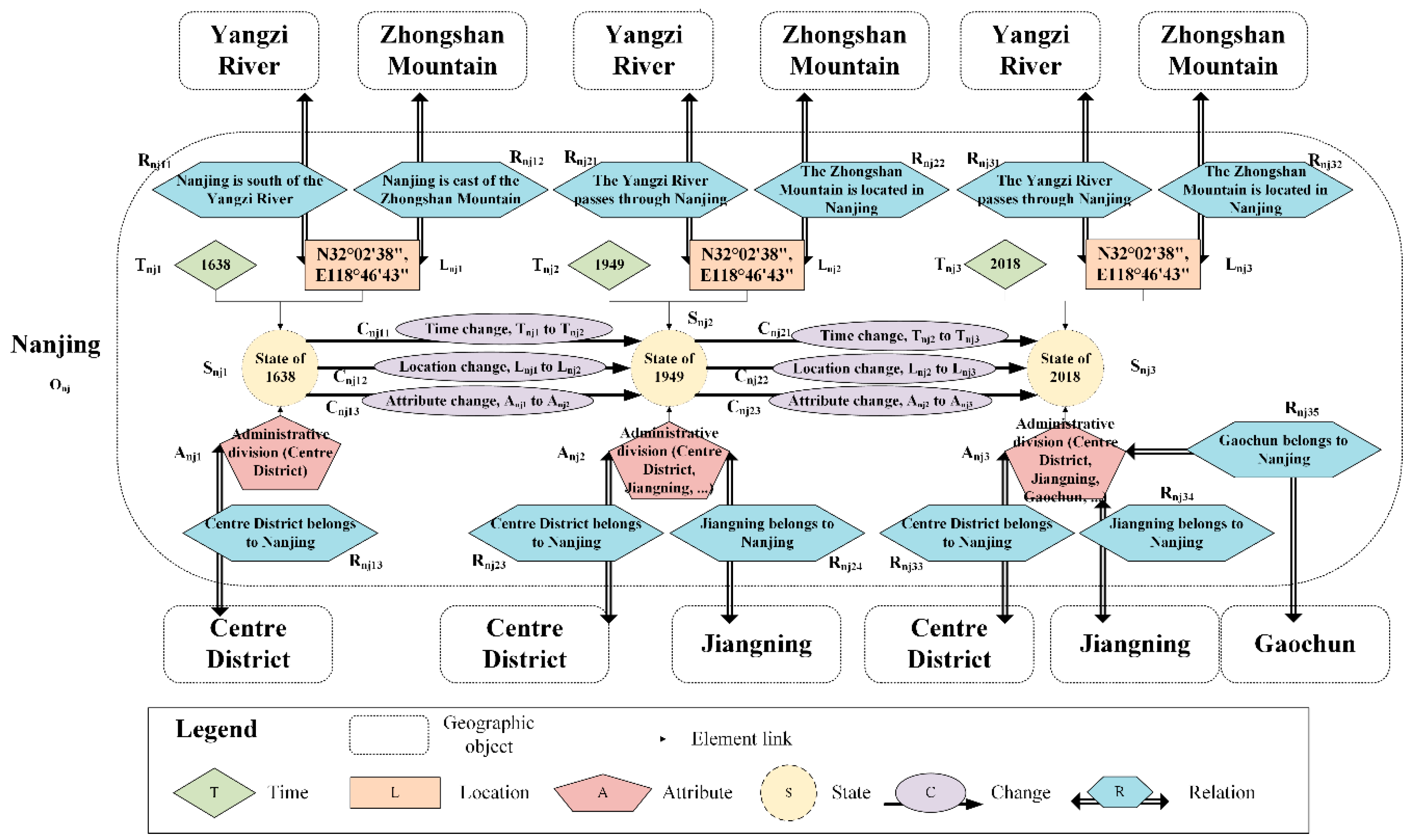
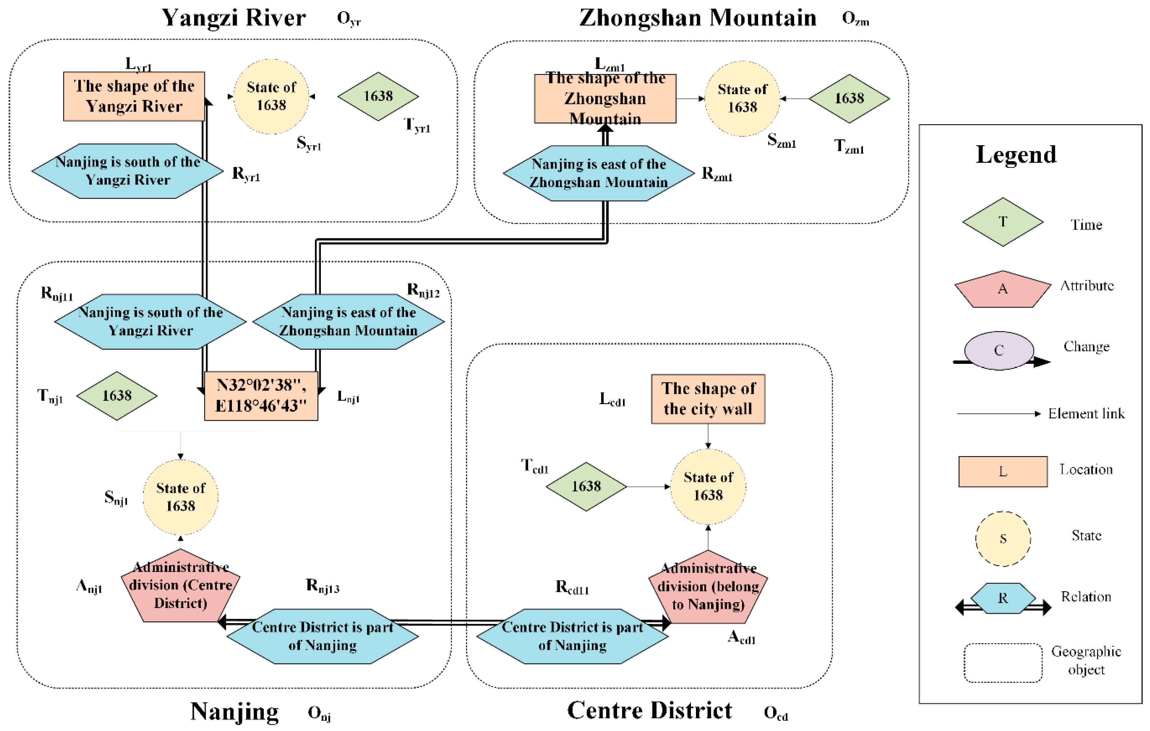
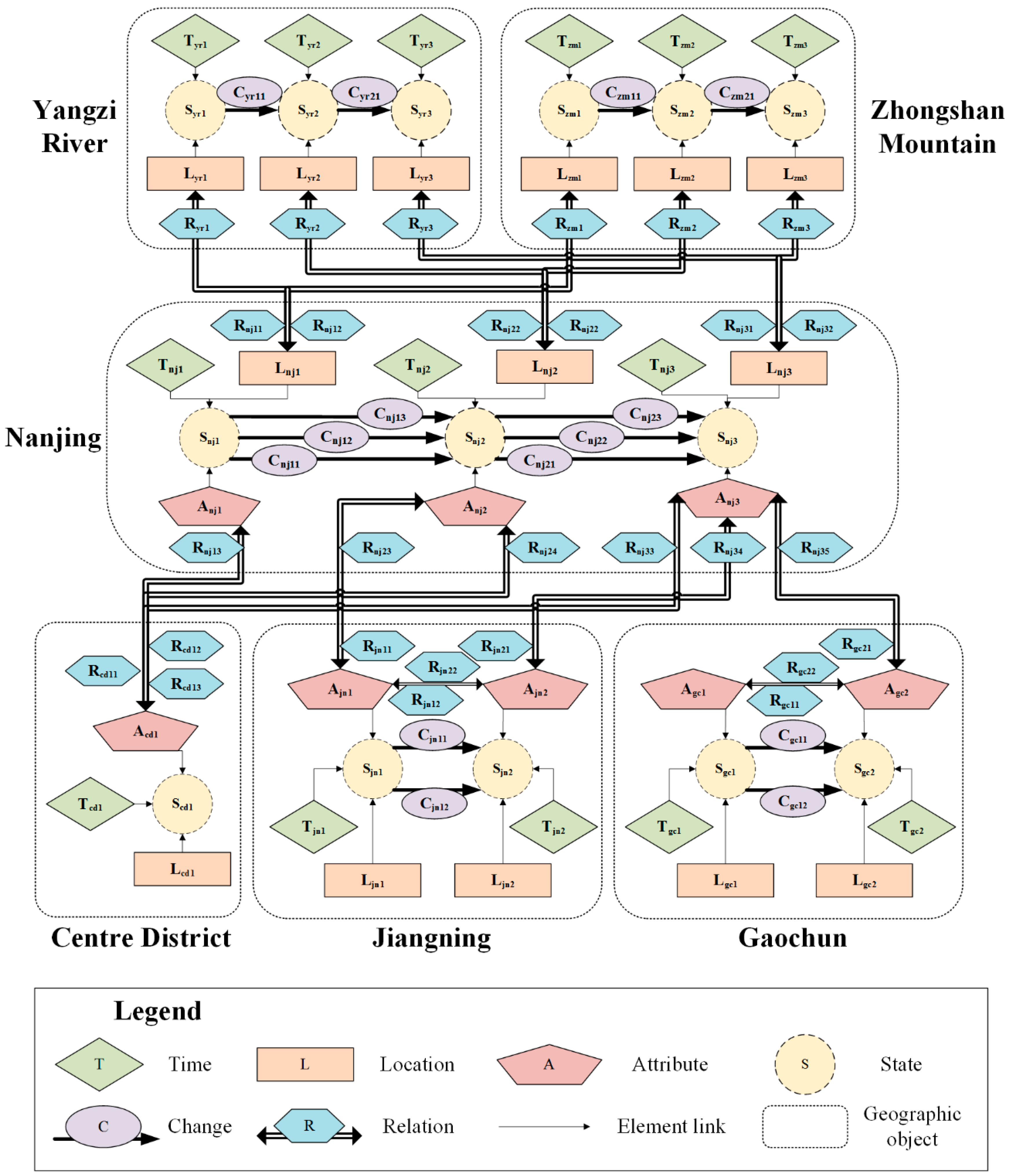
3.1.3. GeoKG Model
3.2. Model Formalization
3.2.1. DL and Construction Operators
3.2.2. Formalization Representation
4. Case Study
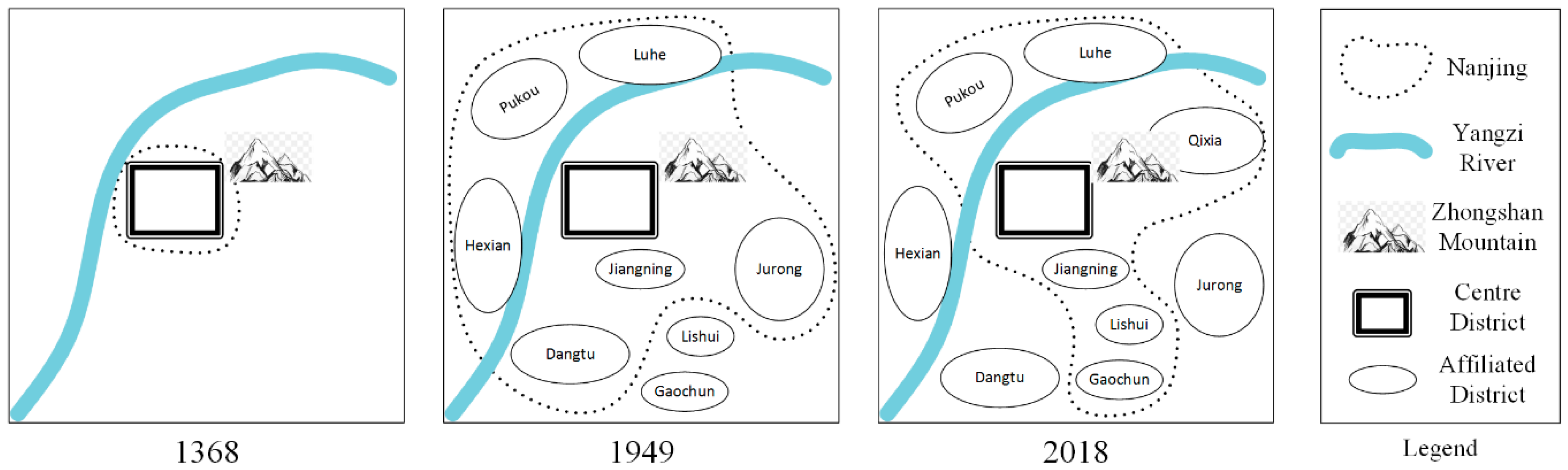
4.1. Research Area
4.2. Formalization
5. Discussion
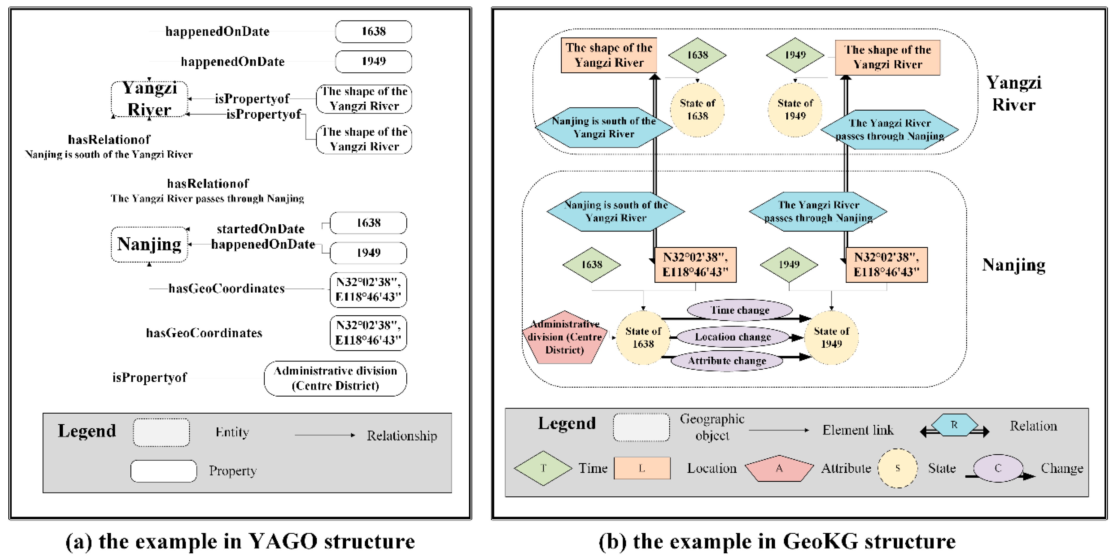
5.1. The GeoKG and the YAGO
5.1.1. Structures
5.1.2. Construction
5.2. The Comparison of Knowledge Representation Ability between the GeoKG and the YAGO
5.2.1. Questions
5.2.2. Queries
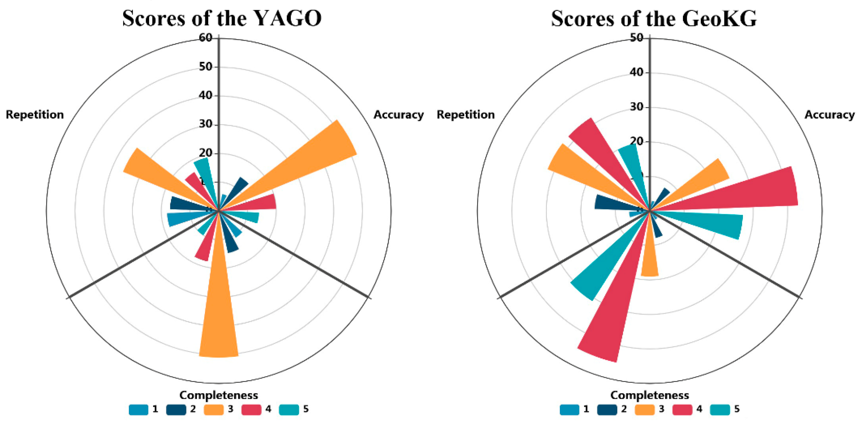
5.2.3. Comparison and Analysis
a. Accuracy
b. Completeness
c. Repetition
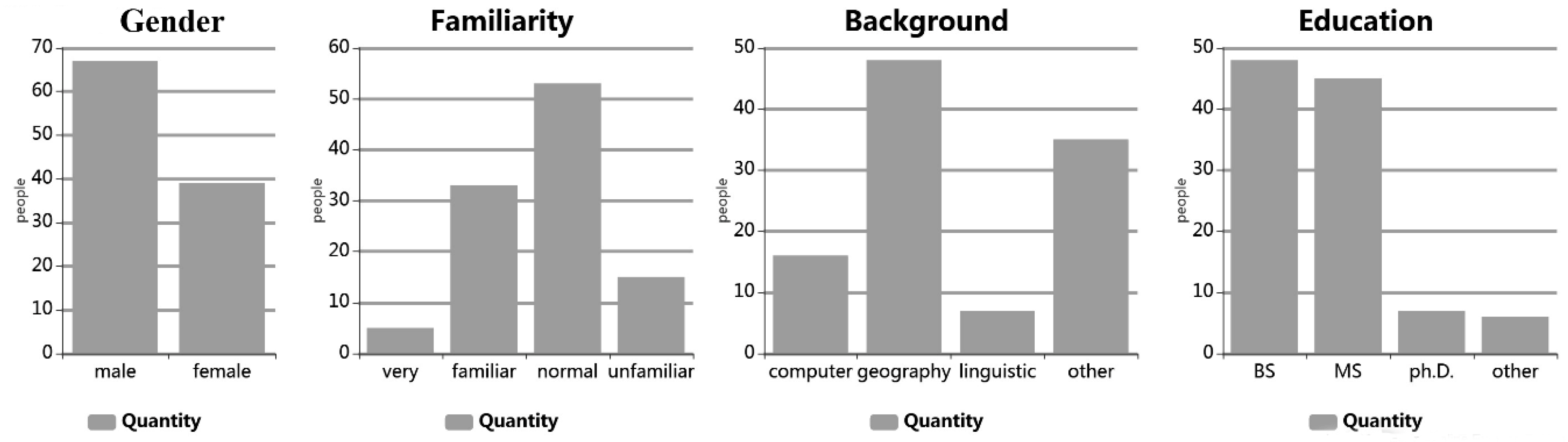
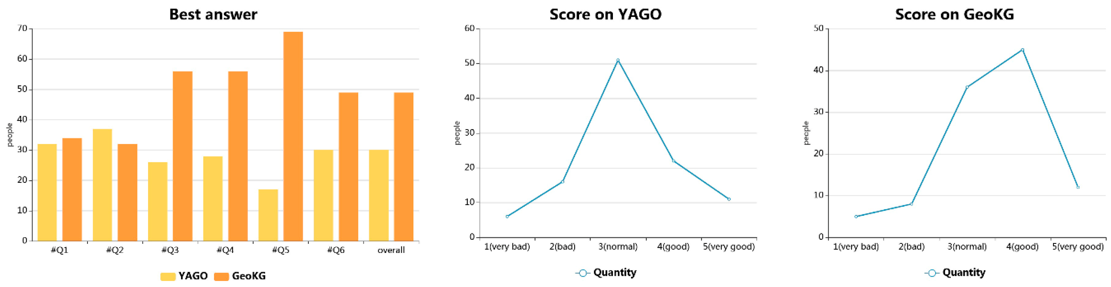
5.2.4. User Evaluation
6. Conclusions
Author Contributions
Acknowledgments
Conflicts of Interest
References
- Golledge, R.G. The Nature of Geographic Knowledge. Ann. Assoc. Am. Geogr. 2015, 92, 1–14. [Google Scholar] [CrossRef]
- Haubrich, H. International Charter on Geographical Education. J. Geogr. 1997, 96, 33–39. [Google Scholar]
- Davis, R. What Is a Knowledge Representation? AI Mag. 1993, 14, 17–33. [Google Scholar]
- Zhang, Y.; Gao, Y.; Xue, L.L.; Shen, S.; Chen, K. A common sense geographic knowledge base for GIR. Sci. Technol. Sci. 2008, 51, 26–37. [Google Scholar] [CrossRef]
- Kuhn, W. Modeling Vs Encoding for the Semantic Web. Semant. Web 2010, 1, 11–15. [Google Scholar]
- Baader, F.; Sattler, U. An Overview of Tableau Algorithms for Description Logics. Stud. Log. 2001, 69, 5–40. [Google Scholar] [CrossRef]
- Hoffart, J.; Suchanek, F.M.; Berberich, K.; Weikum, G. YAGO2: A spatially and temporally enhanced knowledge base from Wikipedia. Artif. Intell. 2013, 194, 28–61. [Google Scholar] [CrossRef]
- Guarino, N.; Oberle, D.; Staab, S. What Is an Ontology? HHandb. Ontol. 2009, 1–17. [Google Scholar] [CrossRef]
- Ding, Y.; Foo, S. Ontology research and development. Part 1: A review of ontology generation. J. Inf. Sci. 2002, 28, 123–136. [Google Scholar]
- Couclelis, H. Ontologies of geographic information. Int. J. Geogr. Inf. Sci. 2010, 24, 1785–1809. [Google Scholar] [CrossRef]
- Siricharoen, W.V.; Pakdeetrakulwong, U. A Survey on Ontology-Driven Geographic Information Systems. In Proceedings of the Fourth International Conference on Digital Information and Communication Technology and It’s Applications, Bangkok, Thailand, 6–8 May 2014. [Google Scholar]
- Gruber, T.R. Toward principles for the design of ontologies used for knowledge sharing? Int. J. Hum.-Comput. Stud. 1995, 43, 907–928. [Google Scholar] [CrossRef]
- Fonseca, F.T.; Egenhofer, M.J. Ontology-driven geographic information systems. In Proceedings of the 7th ACM International Symposium on Advances in Geographic Information Systems, Kansas City, MO, USA, 2–6 November 1999; Volume 71, pp. 14–19. [Google Scholar]
- Jun, X.U.; Tao, P.; Yao, Y. Conceptual Framework and Representation of Geographic Knowledge Map: Conceptual Framework and Representation of Geographic Knowledge Map. J. Geo-Inf. Sci. 2010, 12. [Google Scholar] [CrossRef]
- Chen, J.; Deng, S.; Chen, H. Crowdgeokg: Crowdsourced Geo-Knowledge Graph. In Proceedings of the China Conference on Knowledge Graph and Semantic Computing, Chengdu, China, 26–29 August 2017. [Google Scholar]
- Arvor, D.; Durieux, L.; Andrés, S.; Laporte, M.-A. Advances in Geographic Object-Based Image Analysis with ontologies: A review of main contributions and limitations from a remote sensing perspective. ISPRS J. Photogramm. Remote. Sens. 2013, 82, 125–137. [Google Scholar] [CrossRef]
- Brown, S.H. Knowledge Representation and the Logical Basis of Ontology; Springer: London, UK, 2012; pp. 11–50. [Google Scholar]
- Pittet, P.; Cruz, C.; Nicolle, C. Modeling Changes for Shoin(D) Ontologies: An Exhaustive Structural Model. In Proceedings of the IEEE Seventh International Conference on Semantic Computing, Irvine, CA, USA, 16–18 September 2013. [Google Scholar]
- Sattler, U.; Horrocks, I. A description logic with transitive and inverse roles and role hierarchies. J. Log. Comput. 1999, 9, 385–410. [Google Scholar] [CrossRef]
- Horrocks, I.; Sattler, U.; Tobies, S. Practical Reasoning for Expressive Description Logics. In Proceedings of the International Conference on Logic for Programming and Automated Reasoning, Tbilisi, Georgia, 6–10 September 1999. [Google Scholar]
- Horrocks, I.; Sattler, U.; Tobies, S. Practical reasoning for very expressive description logics. Log. J. IGPL 2000, 8, 239–263. [Google Scholar] [CrossRef]
- Aachen, R.; Informatik, L.T.; Horrocks, I.; Sattler, U.; Tobies, S. Pspace-Algorithm for Deciding Alcnir+-Satisfiability. In LTCS-Report 98-08; ACM Digital Library: Aachen, Germany, 1998. [Google Scholar]
- Mei, J. From Alc to Shoq(D):A Survey of Tableau Algorithms for Description Logics. Comput. Sci. 2005, 32, 1–11. [Google Scholar] [CrossRef]
- Singhal, A. Official Google Blog: Introducing the Knowledge Graph: Things, Not Strings; Northwestern University: Evanston, IL, USA, 2012. [Google Scholar]
- Suchanek, F.M.; Kasneci, G.; Weikum, G. Yago: A Core of Semantic Knowledge. In Proceedings of the 16th International Conference on World Wide Web (WWW), Banff, AB, Canada, 8–12 May 2007; Volume 272, pp. 697–706. [Google Scholar]
- Bollacker, K.; Cook, R.; Tufts, P. Freebase: A Shared Database of Structured General Human Knowledge. In Proceedings of the AAAI Conference on Artificial Intelligence, Vancouver, BC, Canada, 22–26 July 2007. [Google Scholar]
- Wu, W.; Li, H.; Wang, H.; Zhu, K.Q. Probase: A Probabilistic Taxonomy for Text Understanding. In Proceedings of the 2012 ACM SIGMOD International Conference on Management of Data (SIGMOD’12), Scottsdale, AZ, USA, 20–24 May 2012. [Google Scholar]
- Lehmann, J. Dbpedia: A Large-Scale, Multilingual Knowledge Base Extracted from Wikipedia. Semant. Web 2015, 6, 167–195. [Google Scholar]
- Li, J.; Liu, R.; Xiong, R. A Chinese Geographic Knowledge Base for Gir. In Proceedings of the IEEE International Conference on Computational Science and Engineering, Guangzhou, China, 21–24 July 2017. [Google Scholar]
- Kauppinen, T.; Espindola, G.M. Ontology-Based Modeling of Land Change Trajectories in the Brazilian Amazon. In Proceedings of the Geoinformatik, Münster, Germany, 15–17 June 2013. [Google Scholar]
- Zhu, Y.; Zhou, W.; Xu, Y.; Liu, J.; Tan, Y. Intelligent Learning for Knowledge Graph towards Geological Data. Sci. Program. 2017, 2017, 1–13. [Google Scholar] [CrossRef]
- William, M. (Ed.) The American Heritage Dictionary of the English Language; New College Edition; Houghton Mifflin Company: Boston, MA, USA, 1980. [Google Scholar]


| Category (Symbol) | Construction Operators | Syntax | Semantics | Diagrams | Category (Symbol) | Construction Operators | Syntax | Semantics | Diagrams |
|---|---|---|---|---|---|---|---|---|---|
| ALC | Top concept |  | ALC | Value restriction |  | ||||
| Bottom concept |  | H | Concept inclusion |  | |||||
| Atomic concept |  | Role inclusion |  | ||||||
| Atomic role |  | I | Inverse role |  | |||||
| Conjunction |  | Trans role |  | ||||||
| Disjunction |  | Q | Qualifying at least restriction |  | |||||
| Negation |  | Qualifying at most restriction |  | ||||||
| Exist restriction |  |
| Question Types | Factual Question | Inferential Question |
|---|---|---|
| Time | When was Nanjing named? | When does Jiangning belong to Nanjing? |
| Space | Where is Nanjing? | What is the spatial relationship between Nanjing and Yangzi River? |
| Attribute | Which city does Gaochun belong to? | What administrative divisions belong to Nanjing? |
| Steps | SPARQL Query | Semantic Meaning |
|---|---|---|
| 1 | PREFIX rdfs: <http://www.w3.org/2000/01/rdf-schema#>. | protocol |
| 2 | SELECT ?sTime WHERE { | Query content “?sTime” (start time) |
| 3 | ?s rdfs:type :City. | Type is “City” |
| 4 | ?s :cityName ‘Nanjing’. | Get “Nanjing” geographic object |
| 5 | ?s :hasName ?o. | Get time when named ‘Nanjing’ |
| 6 | ?o :startedOnDate ?sTime. | Get started time |
| 7 | ?o :usedName ?uName. | Constraint condition |
| 8 | FILTER regex(?uName, “^Nanjing”) | Constraint condition setting |
| } |
| Question Types | Questions | Results | |
|---|---|---|---|
| YAGO | GeoKG | ||
| Time | #Q1: When was Nanjing named? |
|
|
| #Q2: When does Jiangning belong to Nanjing? |
|
| |
| Space | #Q3: Where is Nanjing? |
|
|
| #Q4: What is the spatial relationship between Nanjing and Yangzi River? |
|
| |
| Attribute | #Q5: Which city does Gaochun belong to? |
|
|
| #Q6: What administrative divisions belong to Nanjing? |
|
| |
© 2019 by the authors. Licensee MDPI, Basel, Switzerland. This article is an open access article distributed under the terms and conditions of the Creative Commons Attribution (CC BY) license (http://creativecommons.org/licenses/by/4.0/).
Share and Cite
Wang, S.; Zhang, X.; Ye, P.; Du, M.; Lu, Y.; Xue, H. Geographic Knowledge Graph (GeoKG): A Formalized Geographic Knowledge Representation. ISPRS Int. J. Geo-Inf. 2019, 8, 184. https://0-doi-org.brum.beds.ac.uk/10.3390/ijgi8040184
Wang S, Zhang X, Ye P, Du M, Lu Y, Xue H. Geographic Knowledge Graph (GeoKG): A Formalized Geographic Knowledge Representation. ISPRS International Journal of Geo-Information. 2019; 8(4):184. https://0-doi-org.brum.beds.ac.uk/10.3390/ijgi8040184
Chicago/Turabian StyleWang, Shu, Xueying Zhang, Peng Ye, Mi Du, Yanxu Lu, and Haonan Xue. 2019. "Geographic Knowledge Graph (GeoKG): A Formalized Geographic Knowledge Representation" ISPRS International Journal of Geo-Information 8, no. 4: 184. https://0-doi-org.brum.beds.ac.uk/10.3390/ijgi8040184