On the Feasibility of Water Surface Mapping with Single Photon LiDAR


1
Institute for Photogrammetry, University of Stuttgart, 70174 Stuttgart, Germany
2
TU Wien, Department of Geodesy and Geoinformation, 1040 Vienna, Austria
3
Karlsruhe Institute of Technology (KIT), Institute of Photogrammetry and Remote Sensing, 76131 Karlsruhe, Germany
*
Author to whom correspondence should be addressed.
ISPRS Int. J. Geo-Inf. 2019, 8(4), 188; https://0-doi-org.brum.beds.ac.uk/10.3390/ijgi8040188
Submission received: 9 February 2019
/
Revised: 25 March 2019
/
Accepted: 1 April 2019
/
Published: 10 April 2019
(This article belongs to the Special Issue Innovative Sensing - From Sensors to Methods and Applications)
Abstract
:Single photon sensitive airborne Light Detection And Ranging (LiDAR) enables a higher area performance at the price of an increased outlier rate and a lower ranging accuracy compared to conventional Multi-Photon LiDAR. Single Photon LiDAR, in particular, uses green laser light potentially capable of penetrating clear shallow water. The technology is designed for large-area topographic mapping, which also includes the water surface. While the penetration capabilities of green lasers generally lead to underestimation of the water level heights, we specifically focus on the questions of whether Single Photon LiDAR (i) is less affected in this respect due to the high receiver sensitivity, and (ii) consequently delivers sufficient water surface echoes for precise high-resolution water surface reconstruction. After a review of the underlying sensor technology and the interaction of green laser light with water, we address the topic by comparing the surface responses of actual Single Photon LiDAR and Multi-Photon Topo-Bathymetric LiDAR datasets for selected horizontal water surfaces. The anticipated superiority of Single Photon LiDAR could not be verified in this study. While the mean deviations from a reference water level are less than 5 cm for surface models with a cell size of 10 m, systematic water level underestimation of 5–20 cm was observed for high-resolution Single Photon LiDAR based water surface models with cell sizes of 1–5 m. Theoretical photon counts obtained from simulations based on the laser-radar equation support the experimental data evaluation results and furthermore confirm the feasibility of Single Photon LiDAR based high-resolution water surface mapping when adopting specifically tailored flight mission parameters.
1. Introduction
Precise knowledge of area-wide water surface heights is inevitable for many disciplines such as hydrology, hydraulic engineering, flood risk management, ecology, climate change, etc. [1,2,3,4]. In hydro sciences, continuous water level heights are required as ground truth for calibrating and validating rainfall-runoff models [5] and multidimensional hydrodynamic-numerical models, also referred to as computational fluid dynamic (CFD) models. Multidimensional CFD models require a spatially continuous description of the water bottom geometry as basic input and extensive water surface levels for calibration. On the one hand, a large body of literature exists for capturing the bottom of coastal and inland waters using optical remote sensing from airborne and spaceborne platforms such as multimedia photogrammetry [6,7], spectrally-based depth estimation [8,9], and laser bathymetry [10,11,12], but on the other hand comparably few studies focus on high-resolution mapping of the water surface itself [13,14].
However, sub-dm water level height accuracy is not only required for estimating global water level rise [14] and for bathymetric Light Detection And Ranging (LiDAR) as the precondition for proper refraction correction of the raw signal [10,15,16], but also, as mentioned above, for calibration and validation of multidimensional CFD models. Such models allow simulation of realistic and complex flow situations including, for example, a potential surface tilt for bended rivers. Spatially static gauge measurements alone, however, do not provide sufficient information for hydraulic model calibration. Topographic airborne LiDAR potentially delivers spatially distributed water surface height measurements, but surface returns can only be expected in a small angle range around the nadir direction [17], and off-nadir angles larger than 5–7 lead to laser drop-outs [13].
The recent advent of LiDAR sensors using low-energy pulses and single photon sensitive detectors in the commercial market has increased the areal coverage performance compared to conventional LiDAR sensors [18] at the price of a reduced ranging accuracy and a higher measurement noise [19,20]. In particular the technology commonly referred to as Single Photon LiDAR, originally developed by Sigma Space Corporation and now available as a Leica/Haxagon product (SPL100), is suitable for both area-wide topographic mapping and derivation of shallow water bathymetry [21].
In this contribution, we investigate the capability of Single Photon LiDAR operating with very short laser pulses (400 ps) in the visible green domain of the spectrum ( = 532 nm) for large-area water surface mapping. For this purpose, the use of the water-penetrating green wavelength entails additional complexity compared to infrared wavelengths used for topographic mapping [22]. Therefore, the specific research questions are (i) if the single photon sensitivity results in sufficiently many echoes to enable high-resolution water surface mapping, and (ii) if water surface level underestimation is less compared to conventional LiDAR. The underestimation effect is well known from literature for green laser radiation [1,3,23]. In addition, we investigate (iii) whether the flight mission parameters generally optimized for topographic mapping are equally suitable for water surface detection, or otherwise, which settings need to be adapted to enable high-resolution water level mapping.
We address the topic from a theoretical point of view based on the laser-radar equation and empirically by comparing Single- and Multi-Photon LiDAR point clouds of selected horizontal water bodies such as reservoirs or ponds. Being aware that different types of Single Photon LiDAR technologies exist and that the same also applies to conventional LiDAR, often referred to as linear mode LiDAR [22], we deliberately chose the above notation. In both cases, ranging is performed by measuring the round-trip time of short laser pulses, and the systems only differ w.r.t. detector sensitivity and signal processing. Thus, the employed terminology does not aim to introduce a new categorization, but should rather highlight that either a few or hundreds of photons are necessary for object detection.
The remainder of this article is structured as follows. Section 2 introduces the basics of Multi- and Single Photon LiDAR (Section 2.1) and reviews the interaction of laser light with the medium of water (Section 2.2). In Section 3, the study areas and data processing steps are presented. The results of the case study are presented and interpreted in Section 4, and Section 5 discusses the data evaluation results and connects them to the theory presented before. Section 6, finally, summarizes the main findings and provides an outlook on future research.
2. Basics of LiDAR Technology
In this section, we briefly review the basics and specific differences of conventional Multi-Photon LiDAR and recent Single Photon LiDAR together. Furthermore, we revisit the interaction of green laser light with the medium water and thereby verify the general feasibility of using Single Photon LiDAR for water surface mapping.
2.1. Multi-Photon vs. Single Photon LiDAR Technology
In this contribution, point clouds derived from conventional Multi-Photon LiDAR are compared against recent Single Photon LiDAR technology. For a better understanding of the data recording, the specifications of established conventional Multi-Photon LiDAR in general and a specific Topo-Bathymetric LiDAR system (RIEGL VQ-880-G) in particular are presented and compared with Single Photon LiDAR (Leica/Hexagon SPL100). The presented specifications in Table 1 base on company brochures [24,25], internet research, or literature [18,21,26].
The Multi-Photon LiDAR point clouds are captured with a Topo-Bathymetric LiDAR system (RIEGL VQ-880-G). While this instrument records the full-waveform profile of each backscattered laser pulse with 2 GHz enabling sophisticated offline waveform analysis in postprocessing, the system also performs online waveform processing [27]. In the latter case, the received waveform is analyzed in real time and the shape of the waveform in the vicinity of a local maximum is evaluated in detail. Next to the raw amplitude A and range R, the following quantities are provided for each echo: (i) calibrated amplitude (i.e., amplitude measure [dB] proportional to the instrument’s detection limit), (ii) relative reflectance (i.e., difference [dB] between the measured amplitude and the theoretical amplitude of a diffusely reflecting object with known reflectivity at a distance of R), and (iii) pulse shape deviation (i.e., a measure describing the deviation of the measured echo pulse from an ideal single object return with orthogonal incidence of the laser beam).
In general, the Single Photon LiDAR technology implemented in the Hexagon/Leica SPL100 is characterized by two essential optical components: (i) a Diffractive Optical Element (DOE) splitting the laser beam into an array of 10 × 10 beamlets and (ii) an Optical Receiver consisting of photosensitive sub-arrays, where each sub-array is aligned to a beamlet and contains numerous photosensitive detector elements. These optical components ensure an efficient illumination of the photosensitive sub-array and additionally avoid optical crosstalk.
- (I)
- By the Diffractive Optical Element an array of 10 × 10 beamlets is provided. For a single beamlet, the given beam divergence of 0.08 mrad is supposed to merge approximately the instantaneous FoV (iFoV) of the relevant photosensitive sub-array with numerous detector elements (sometimes called micro-cells) as depicted in Figure 1. The iFoV is adjustable to a certain degree, but the exact size is not specified by the manufacturer. It is furthermore noted that beam splitting is not restricted to using DOEs but can also be achieved, e.g., with a microlens array.
- (II)
- The Optical Receiver consists of hundreds of photosensitive detector elements enabling multiple single photon detection, usually referred to as pixelated array detector. While the applied technology is not disclosed by the manufacturer, Micro Channel Plate PhotoMultiplier Tubes (MCP-PMT, [28]), Silicon PhotoMultipliers (SiPM, [29]), or Single Photon Avalanche Diode (SPAD, [30,31]) arrays are more or less suitable. The very low jitter of the detector element is sometimes specified by the companies with 50–100 ps (is equivalent to 0.75–1.5 cm in range), which has a significant impact on the ranging accuracy. Furthermore, a low recovery time (1.6 ns is equivalent to 24 cm in range) is important for daytime measurement capability as reflections from the laser or sun light at particles in the atmosphere may trigger detection events. The low recovery time essentially enables multi-target capabilities and allows promising vegetation and bathymetry measurements. For the presented study, this is especially important for water surface detection beneath littoral vegetation.
The Single Photon LiDAR instrument SPL100 from Leica/Hexagon operates with a wavelength of 532 nm. While this visible green wavelength generally exhibits low reflectance values for natural surfaces (soil/dry vegetation 15% and green vegetation 10%), it is advantageous for LiDAR because the optical components are inexpensive, the detector elements show a high efficiency, detector dark count contributions to background noise are typically much lower and the good transmission characteristic in water supports topographic as well as bathymetric mapping with a single instrument [21].
Furthermore, the instrument design is optimized to gain a maximum point density. The Single Photon LiDAR is tuned for per-pixel Photon Detection Efficiency (PDE) of 0.95 for a 10% surface reflectance (e.g., green vegetation) and a PDE of 0.99 for a 15% surface reflectance (e.g., soil/dry vegetation) [21]. With a maximum flying height of 4500 m AGL (Above Ground Level), the areal coverage of Single Photon LiDAR is higher compared to lower altitude Multi-Photon LiDAR, while delivering comparable point densities (typically: 8–15 points/m). Figure 2 depicts exemplary the returns of three consecutive SPL100 laser pulses, demonstrating the scan grid resulting from the regular array of 100 beamlets per laser pulse.
In the aquatic domain, the water surface itself, the submerged water bottom, and the dry ground surface in the littoral area are challenging to measure with a LiDAR in a single campaign. Considering the short laser pulse width (400 ps is equivalent to 6 cm in range) and the short jitter interval (50–100 ps is equivalent to 0.75–1.5 cm range) for Single Photon LiDAR, an accurate surface ranging can be expected for the water level as well as for the (shallow) water bottom with the first photon detection. In comparison, for Multi-Photon LiDAR the laser pulse width (1–5 ns is equivalent to 15–75 cm in range) is much greater and waveform processing is challenging [32,33] especially due to the different speed of light in the medium air and water. Even if the first photon detection for Single Photon LiDAR is not caused by the water surface, it is likely that a measurement is derived from the water column below the water surface or the water bottom. For second photon detection the low recovery time of Single Photon LiDAR is obviously relevant and the main limiting issue for separating individual objects.
It is noted here that, although both Multi-Photon LiDAR and Single Photon LiDAR in general and the respective instruments used in this investigation (VQ-880-G, SPL100) in particular provide signal strength information, the investigation at hand entirely focuses on the geometry of the obtained discrete-echo point clouds.
2.2. Laser Light Interaction with Water
The study at hand bases on the assumption that at least a few photons are scattered back from the air–water interface and the first cm of the water column, enabling water surface detection with a Single Photon LiDAR sensor. Before addressing this question empirically using measured data, we briefly review the theoretical basis of the interaction of green laser light with the medium water to back up the general practicability w.r.t. mapping of water surfaces and shallow water bathymetry. All numbers presented in this subsection are calculated for the SPL100 instrument and the respective parameters are taken from the sensor’s data sheet [24] and from literature.
We start with the estimation of the number of transmitted photons per beamlet which are related to the average optical output power , the transmitted pulse energy , the efficiency of the diffractive optical element , the pulse repetition rate , the number of beamlets , the speed of light c, the laser wavelength , and Planck’s constant h as expressed in Equation (1).
For an average power of 5 W, a of 60 kHz, and a conservatively estimated DOE efficiency of 80% this results in roughly transmitted photons for the pulse of a single beamlet at a laser wavelength of 532 nm. The general relation between the transmitted power and the received power is described by the laser-radar equation, which is written in its general form in Equation (2) [34]:
In Equation (2), D denotes the diameter of the receiver aperture, R the sensor-to-target distance, and the laser beam divergence. Power losses from the system and atmosphere are described by the two transmission factors and and the target properties are summarized in the backscattering cross-section .
incorporates the illuminated area A (respectively laser footprint on the ground), the backscattering angle , and material properties (respectively reflectance). A perfect diffuse (i.e., Lambertian) reflector is characterized by , whereas small values of near zero denote specular reflection typical for calm water surfaces.
The entire atmospheric correction for the round trip of the laser signal can be calculated as described in [35]:
In Equation (4), denotes the atmospheric attenuation coefficient in [dB/km] and R the measurement range in [m]. For wavelengths in the green domain of the spectrum and for clear atmosphere (i.e., visibility: 15 km), amounts to 0.25 [36] resulting in a total atmospheric transmission of 63.1% for a range of 4 km.
While this generic formulation of the laser-radar equation is mainly used to describe scattering from simple targets, the interaction of green laser radiation with water in general and with the water surface in particular is more complex. To further estimate the amount of optical power scattered from the air–water interface and the first cm of the water column, we use the formulation of the laser-radar equation describing bathymetric waveforms [37,38]:
Equation (5) separates the echo signal received from a green laser pulse hitting water into contributions from the water surface , the water column , and the water bottom , while denotes the power of the background light. For our purpose we are mainly interested in the surface response .
In Equation (6), denotes the loss of transmission through the surface, also referred to as surface albedo. Based on the geometric model of [39], is calculated by the bidirectional reflectance distribution function (BRDF) of the water surface represented by micro-facets:
Therein, and denote the degree of specular and diffuse reflection, respectively, which together sum up to 1 (). O represents the geometric BRDF attenuation factor, a function describing the Fresnel reflection of light on each micro-facet, and the micro-facet slope distribution function according to [40]:
High values of r (e.g., >0.5 ) represent rough water surface conditions, which reduce the specular component increasing the probability for detecting water surface echoes. Laser beam directions around the nadir direction, in turn, result in small incidence angles , which increase the chance for capturing specular reflections at the receiver.
For small incidence angles, is a function of the refractive indices in air () and water (), respectively, and can be calculated as:
In addition to the reflection from the water surface, green laser radiation also penetrates the water column, where diffuse volume backscattering at small floating or suspended particles occurs. Therefore, we include the contribution of the very first part of the water column in our considerations, which can be written as reported in [37]:
F is a loss factor due to the limited field of view of the telescope, is the volume scattering function, is the traveling distance within the water column, the refractive index of water, and k the diffuse attenuation coefficient describing the degradation rate of light in water.
As expressed above, scattering at the air–water interface is generally characterized by a high degree of specular reflection ( 0.9). Smooth water surface characteristics and large laser incidence angles result in low scattering back to the direction of the receiver. Within the water column, turbidity represented by higher k-values (clear: k = 0.2, average: k = 1, turbid: k > 1) limit the penetration depth [41], but the higher degree of volume backscattering also increases the signal level from the first few mm of the water column. A comprehensive discussion of the interaction of laser radiation with water can be found in [17].
We conclude the theory section by evaluating Equations (6) and (10) for representative scenarios and reporting the calculated values in Table 2. The last column contains the estimated number of photons scattered back to the receiver for the SPL100 sensor [24]. Keeping in mind from Equation (1) that there is a direct relation between the optical power and the photon count, the latter is reported in Table 2 rather than the actual received power .
All calculations are carried out for = transmitted photons per beamlet, a usable receiver aperture diameter D = 4 cm, very clear atmosphere (visibility: 40 km, = 0.1), a system efficiency factor = 0.70, a small subsurface layer of = 2 cm, as well as refractive indexes of air and water, respectively, of = 1.0003 and = 1.33. For the remaining parameters, we use the values reported in [37] (O = F = 1.0, = 0.0014). Furthermore, we assume moderate turbidity (k = 1). In Table 2, denotes the expected number of photons from reflection near the air–water interface as the sum of photons backscattered from the water surface () and the 2 cm water layer ().
3. Materials and Methods
3.1. Study Areas and Datasets
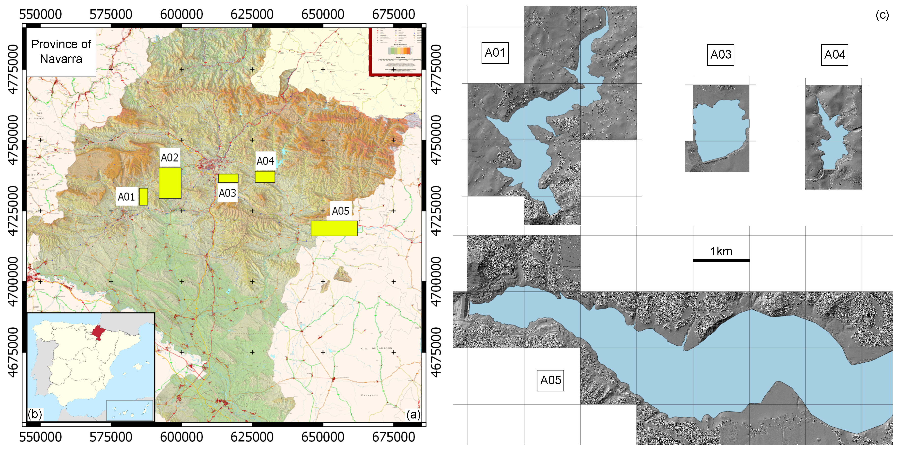
In 2017, the government of Navarra (Spain) commissioned a flight campaign for capturing the entire province area with a Leica SPL100 sensor. From the area-wide dataset, the company Trascasa provided the unfiltered point cloud of six areas featuring different inland water bodies (rivers, reservoirs; cf. Figure 3). It is noted that in the meantime the entire dataset is publicly available via FTP download (ftp://ftp.cartografia.navarra.es/5_LIDAR/5_4_2017_NAV_cam_EPSG25830/). As no external water level reference data were available, four reservoirs with horizontal water level were chosen as the specific study areas (A01, A03–05, cf. Figure 3b,c).
The 3D point clouds were captured from an altitude of about 4200 m AGL. From this flying height, conical scanning (Palmer scanner) with a constant off-nadir angle of 15 (i.e., total scanner FOV = 30) yields a single strip swath width of about 2260 m. Flying at a speed of 90 m/s with an effective scan rate of 6 Mhz (PRR: 60 kHz, 100 beamlets per laser pulse), results in an average last-echo point density on dry ground of 14.5 points/m. Due to the circular scan pattern on the ground, the point density is considerably larger at the strip boundary compared to the strip center. Moreover, for every detected echo the sensor provides the 3D coordinates (x, y, z), the time stamp (t), and additional attributes (signal strength, RGBI, scan angle, etc.). The scanner provides intensity information by summing up the signals from all nearly synchronously triggered micro-cell array elements within the beamlets’ iFoV. Each point is colorized in postprocessing based on the concurrently acquired images from the incorporated RCD30 80 MPix RGBI camera. All mission parameters are additionally listed in Table 3.
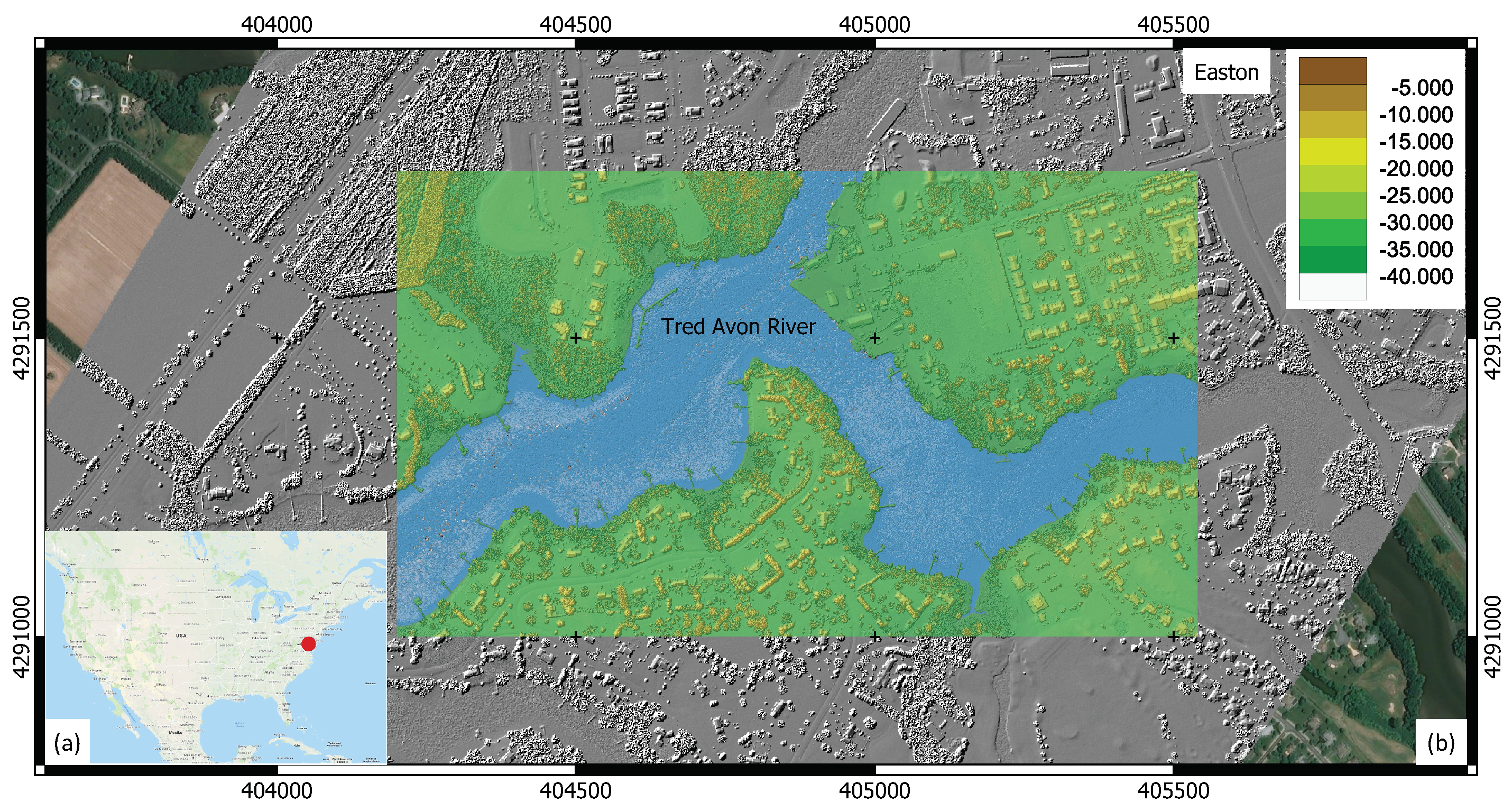
Leica Geosystems provided a second Single Photon LiDAR dataset, acquired on 19 December 2017, in Easton, MD, USA from a flying altitude of 3750 m. A comparable, albeit slightly lower last-echo point density on dry ground of 12 points/m is the result of a lower PRR of 50 Hz, which is compensated by a lower flight velocity (70 m/s). It is noted that in both cases (Navara, Easton), the chosen flight mission parameters lead to the emission of a second pulse, while the return of the first pulse is still in the air, referred to as Multiple Pulses in Air (MPiA). From the provided flight block, a single strip covering the periphery of Easton as well as the Tred Avon River, a tributary of the Choptank River joining the Chesapeak Bay, was selected and analyzed. Figure 4 shows the selected part of the flight strip and the location of the study area plotted on a map of the USA.
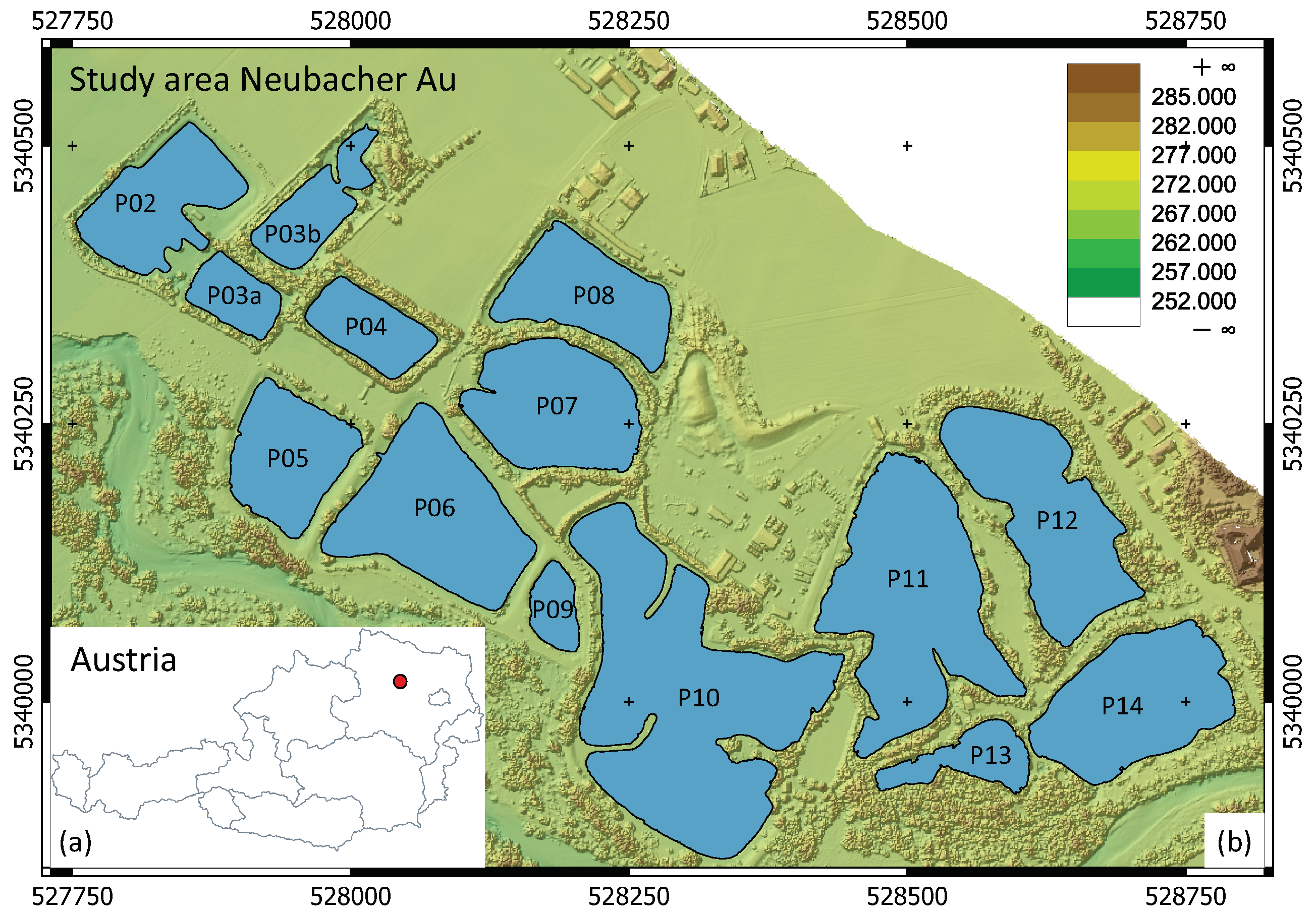
This contribution focuses on the feasibility of Single Photon LiDAR for capturing water surfaces. Due to the lack of independent external reference data, a conventional Topo-Bathymetric dataset captured with a RIEGL VQ-880-G sensor at the Pielach River (Austria) is used as comparison basis. The investigation area (Neubacher Au) is a natural reserve located in the eastern part of Austria (cf. Figure 5). The study reach is repeatedly captured with Topo-Bathymetric LiDAR for monitoring fluvial morphodynamics [42]. Next to the pre-alpine Pielach River, the area features more than a dozen groundwater supplied ponds, each of which exhibiting a constant water level. Data acquisition took place in November 2017 from a flying altitude of 650 m AGL with a flying velocity of 55 m/s. Conical scanning with a constant off-nadir angle of 20 yields a swath width of 480 m. As only a single receiver is employed in this full-waveform instrument, the PRR equals the effective scan rate of 550 kHz. This, however, only leads to a marginally lower point density over land surfaces (14 points/m) compared to the Navarra Single Photon LiDAR dataset. Discrete laser echoes (3D position, attributes: amplitude, reflectance, echo pulse shape deviation) are obtained from online waveform processing [27]. In addition, the waveforms are also stored for offline postprocessing, but this is not employed in investigation at hand. To keep the assessment balanced, the comparison is in both cases conducted based on the discrete-echo point clouds only.
It is stated here that an off-nadir angle of 15–20 is considered the optimum for bathymetric applications [10], thus both systems are well suited for the investigation at hand, as reconstructing the water surface from the measured data is a prerequisite for precise run-time and refraction correction of the water bottom returns [16].
3.2. Data Processing and Assessment Methods
For assessing the suitability of 3D point clouds obtained from Single Photon LiDAR for area-wide water surface mapping, first a couple of preprocessing steps such as quality checks, point cloud filtering, and water-land classification were carried out. Subsequently, a reference water surface level as well as various water surface raster models were determined for each reservoir (Navarra), inlet water body (Easton), and pond (Neubacher Au) based on all points classified as water (water surface, water column, water bottom). Finally, the results were evaluated. The processing steps presented below apply to both Single Photon LiDAR and Multi-Photon LiDAR data acquisition and are based on the strip-wise point clouds.
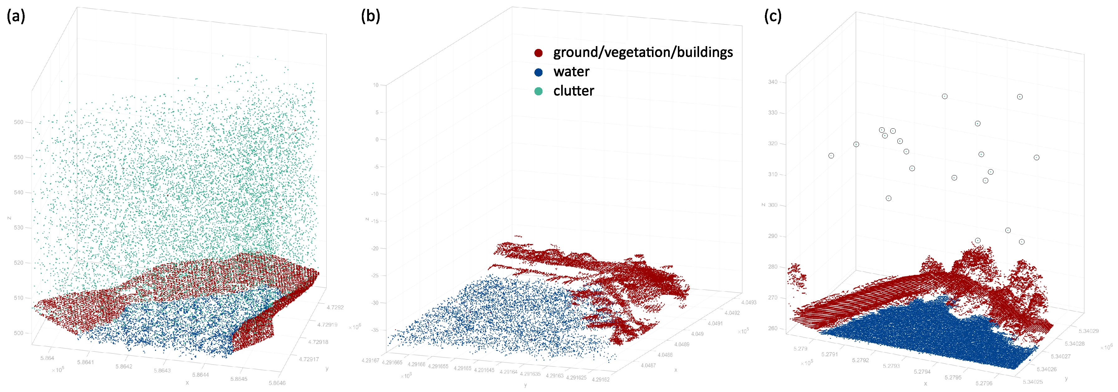
In a preliminary processing step, clutter points above and below the terrain stemming from occasional reflections of the laser pulses at particles in the atmosphere were identified using a volumetric approach. The presence of such points is a general property of Single Photon LiDAR datasets, which is caused by the very high receiver sensitivity. In general, clutter points are characterized by low signal strength and low volumetric point density. For the study at hand, points were classified as clutter if the number of low-intensity laser echoes within a spherical 3 m search radius was below a certain threshold. This requires efficient point handling concerning both geometry and attribute information. The scientific laser scanning software OPALS [43,44] fulfills the aforementioned criteria and was used within this study. It is noted that high-sensitive Multi-Photon LiDAR sensors used for Topo-Bathymetric applications are also prone to deliver clutter points, albeit to a lesser extent. Figure 6 shows representative point clouds from each study area. The Easton dataset does not exhibit clutter points as data delivery only contained the clean, postprocessed points.
In a next step, a standard ALS quality control procedure [43,45] was carried out using the last-echo points to assess (i) the general noise level of the point clouds and the DEMs derived thereof, (ii) the strip fitting precision, and (iii) the achieved point densities. Rating of the noise level and the strip fitting precision was performed by analyzing 0.5 m-DEM raster models interpolated with a moving least squares approach. For each grid post a best fitting plane is estimated from the k-nearest neighbors (k = 15) and the resulting standard deviation of the plane fit () characterizes surface roughness and measurement precision. At smooth surfaces (sealed roads, house roofs, etc.), denotes the spread of the point count cloud (i.e., precision). As reported in Table 3, Multi-Photon LiDAR expectedly outperformed Single Photon LiDAR w.r.t. smoothness (3.0 cm (Navarra) vs. 1.3 cm) and strip fitting precision (3.9/3.0 cm vs. 1.2 cm) due to the shorter ranges and the higher single point reliability being the result of relying on approximately 250 photons for a single range measurement instead of only a few photons in the Single Photon LiDAR case. The Easton study area features a very good local precision of 1.3 cm, competing the Multi-Photon precision level. Prior investigations have already indicated that Single Photon LiDAR exhibits a high precision in the cm range for smooth horizontal surfaces (sealed surfaces), while a higher local spread of the point cloud can be observed for inclined surfaces (e.g., roofs, hill slopes) and natural, grassy surfaces [46]. In general, it can be stated that the overall quality is high for both acquisition methods with strip-to-strip deviations and local precision less than 10 cm.
For deriving a reference water level for each water body (Single Photon LiDAR: reservoirs/ standing river, Multi-Photon LiDAR: ponds), the following two strategies are proposed: Infrared (IR) radiation is strongly absorbed by water, therefore multispectral images are used in literature for Water-Land-Boundary (WLB) delineation [47]. For point clouds derived by Single Photon LiDAR, IR information is available via mapping the colors from the concurrently captured RCD30 images. By interpolating an IR-raster, the WLB is found by deriving the contour line at the appropriate IR-level characterizing the water-land-transition. For standing water bodies, interpolating the heights along this line from the point cloud finally results in a good estimate of the horizontal water level. While this would have been the preferred approach as it allows a fully automated processing chain, it could not be applied to the data at hand due to geometric and radiometric artifacts. The available point colors showed pronounced block effects with the color of water changing from black (as expected for IR) to 75% gray from one processing unit to the next. Furthermore, geometric displacements at block boundaries of up the 2.5 m were detected and prevented the application of the IR-channel-based reference water level estimation.
As an alternative, a first approximate water level was detected interactively by inspecting the 3D point cloud in vertical sections in a 3D data viewer. A value slightly above the actual water level was chosen as green radiation tends to penetrate the topmost level of the water column. This rough estimate allows a first separation into dry and submerged points. The precise water level is subsequently derived as the 99.5% quantile computed from the elevation histogram of all submerged points. This way, occasional points above the water surface (sea birds, boats, littoral area) are filtered out. As no independently measured ground truth was available, the water level determined in such a way serves as the basis for the subsequent evaluation of the individual high-resolution water surface models derived from Single Photon LiDAR and Multi-Photon LiDAR, respectively.
For the derivation of Digital Water Surface Models (DWSM) in regular grid structure with 1 m, 2 m, 5 m, and 10 m grid spacing, we follow the statistical approach of [3]. In each cell, the approach accumulates all submerged points with a maximum water depth of 50 cm and calculates the elevation histogram. Different models, each using a specific quantile (90%, 95%, 98%, 99%, 100%), are calculated and evaluated against the reference water level by computing Digital Elevation Models of Differences (DoD) storing the height difference between the reference level and the estimated cell level. Please note that we use the acronym DoD in this article as it is a common term in the geo-morphology community despite being also used in the LiDAR industry for abbreviating the U.S. Department of Defense. While it is clear that this rather straightforward approach is only applicable to water bodies with horizontal water surface, it still allows addressing the tackled research question of the feasibility of Single Photon LiDAR for water surface mapping when selecting appropriate water bodies. This is definitely the case for the chosen dammed reservoirs (Single Photon LiDAR, Navarra, Spain) and the ground water ponds (Multi-Photon LiDAR/Topo-Bathymetric, Neubacher Au, Austria).
4. Results
In this section, the results of the evaluation methods described in the Section 3.2 applied to the Single Photon LiDAR and Multi-Photon LiDAR datasets introduced in Section 3.1 are presented. After discussing the data preprocessing steps and the overall data quality in Section 4.1, the qualitative and quantitative assessments described in Section 4.2 and Section 4.3, respectively, provide insights on the feasibility and potential restrictions of Single Photon LiDAR for high-resolution water surface mapping. The aim of comparing Single- and Multi-Photon LiDAR datasets is to better understand the properties of the underlying techniques w.r.t. the detection of weakly and often specularly reflecting targets rather than juxtaposing the respective technologies.
4.1. Data Preprocessing
As described in Section 3.2, the processing pipeline started with the detection and classification of clutter points stemming from reflections of the laser signal at aerosol particles in the atmosphere and a raw separation of submerged and dry area. In Figure 6, the resulting 3D point clouds of the Single Photon LiDAR datasets of Navarra (Spain) and Easton (MD, USA) are plotted together with the Topo-Bathymetric Multi-Photon LiDAR dataset (Neubacher Au, Austria). While the blue and red dots represent potential water points and points from the dry part of the scene (ground, vegetation, buildings, etc.), the green dots denote noisy points caused from the atmosphere. Figure 6a shows a detail of study area A01 and constitutes a representative example of a Single Photon LiDAR point cloud. While there are many clutter points above (but also below) the surface, their distribution is both random and homogeneous, and their spherical density is sparse. The simple volumetric approach classifying points featuring less than two neighbors within a sphere with a radius of 50 cm as clutter points, worked reasonably well for the study at hand. As the main emphasis of the study is on water surface mapping, subsequent dry/wet separation based on the semi-automatic approach described in Section 3.2 potentially re-classified clutter points as water in order to preserve the maximum available information for reconstructing the air–water interface.
Figure 6b, in contrast, does not contain any clutter points as the point cloud was already postprocessed by the data provider (Leica Geosystems). As potential water surface points might have been removed during data cleaning, the results from this dataset for water surface mapping need to be treated with caution. Figure 6c, finally, shows that clutter points are not restricted to Single Photon LiDAR, but do also occur in Multi-Photon LiDAR. This especially applies to Topo-Bathymetric LiDAR, where a high-power laser and sensitive receiver is used to detect weak reflections from the water bottom (cf. Table 1). It is noted that only first echoes are displayed in Figure 6c to preserve clarity. However, the multi-return capability is considerably higher for full-waveform-based Multi-Photon LiDAR compared to Single Photon LiDAR [46].
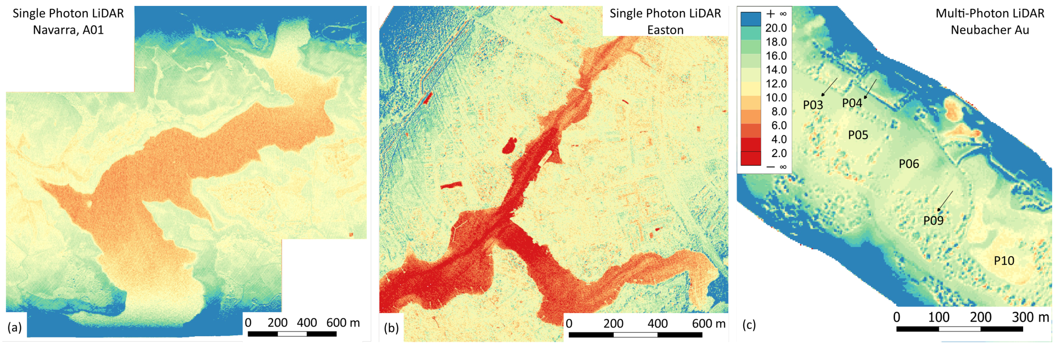
Data preprocessing furthermore contained a full quality check of the strip-wise 3D point clouds including last-echo point-density estimation. Quantitative density estimates are reported in Table 3 separately for water and dry land. In addition, Figure 7 shows the spatially varying point densities as color-coded maps. For the Single Photon LiDAR dataset, test area A01 shows a noticeable point density drop in water of about 50% compared to the surrounding land (land: 14.5 points/m, water: 7 points/m, cf. Table 3), which is representative for all studied Navarra areas. The point density drop is even more pronounced for the Easton dataset (Figure 7b). While, in general, the overall point density is slightly lower for this data acquisition (land: 12.0 points/m), the density drops down to 4.3 points/m in water. We can state that for the analyzed datasets, Single Photon LiDAR exhibits a lower point density over water compared to land. The drop factor varies between 2–2.8 depending on environmental conditions (turbidity, surface roughness, etc.).
The average water point density drop is less for the Multi-Photon LiDAR dataset as can be seen from Figure 7c and Table 3 (land: 14 points/m, water: 12.5 points/m). However, also in this case a considerable density variation can be observed for the individual ponds ranging from almost no (e.g., P04-06) to a pronounced (P07, P10) density drop. This aspect is analyzed and discussed in more detail below. For both Single- and Multi-Photon LiDAR, a much higher point density can be observed at the strip boundary due to the circular scan pattern. While the extreme strip boundary point density (>50 points/m) is unnecessary for capturing topography, it is well advantageous for capturing water surfaces as will be shown subsequently in this section.
4.2. Qualitative Assessment
As introduced in Section 3.2, a representative water level is estimated as the 99.5% elevation quantile of all previously classified water points. This simple strategy is suitable for the selected reservoirs and ponds featuring a constant water level over the entire domain, but it is clear that neither small local water level fluctuations due to wind waves nor running waters can be modeled with this approach. As the main focus of this contribution is to investigate, if the single photon sensitivity results in a more concise response of the green laser signal from the water surface, we concentrate on a qualitative and quantitative assessment of the water level underestimation. The prior is addressed by visual comparison of selected transects (cf. Figure 8) and the latter by evaluating the height differences between the estimated horizontal reference water level and different water surface raster-model variants (cf. Section 4.3).
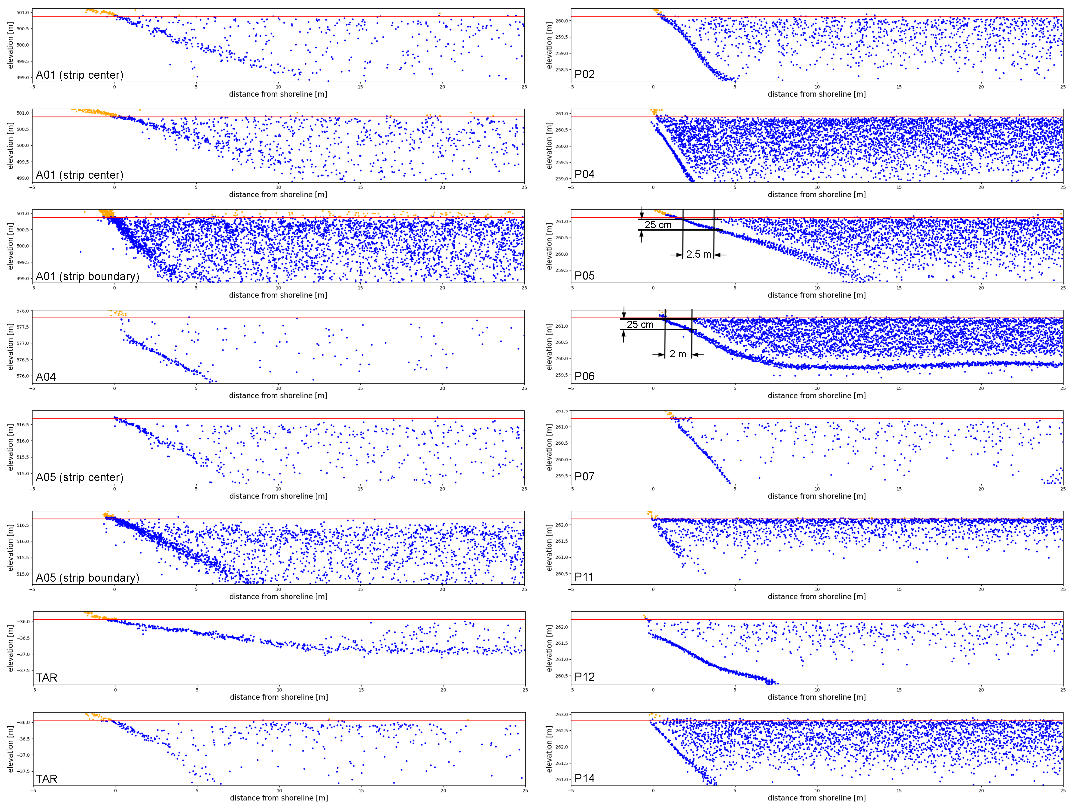
Figure 8 shows point cloud transects in the littoral area of selected Single Photon LiDAR (left) and Multi-Photon LiDAR (right) datasets. Each plot contains the calculated reference water level as a horizontal line (red) and the classified points within a height range of 0.5 m above and 2.0 m below the reference water level (blue: water candidate points, orange: land/vegetation; width of transect: 3 m). The displayed transects reveal variations in overall point density and water level underestimation. The first three examples on the left side, all taken from the same strip of the Single Photon LiDAR area A01, show a gradually increasing density resulting from the respective location of the transect within the flight strip. While the first transect is taken from the center of the strip, the third one is located at the strip boundary where the point density increases dramatically due to the circular scan pattern on the ground (Palmer scanner). While all three examples of area A01 exhibit occasional points on or near the water surface, only the strip boundary transect delivers a dense and continuous coverage with surface echoes. In the same example, the number of (orange) points above the water surface is striking. Due to the single photon sensitivity, there is always a certain probability for early echo detections. Such early detections can also be observed in the middle A01 example, but their frequency is lower due to the lower overall point density. The two examples from area A05 further confirm the argument from above concerning the dependency of the water point density from the overall laser pulse density.
In addition, area A04 is an example of a water body featuring a generally low water point density as a consequence of the very clear water conditions (i.e., low amount of volume scattering). This also applies to the Tred Avon River (TAR) examples (Easton), where the general absence of water surface and water-column points in the shallow water domain (depth < 1 m) are remarkable. Whether no echoes have been detected in this case or usable points were eliminated during postprocessing cannot be answered from the given data. The shown examples indicate a direct relationship between turbidity and discrete-echo point density. However, reliable statements in this respect, especially in the context of Single Photon LiDAR, would need in-depth investigations and are not further discussed here.
In none of the Single Photon LiDAR transects drawn on the left side of Figure 8, the water surface appears as a clear and distinct line of points but reflections from the surface and the water column are rather about uniformly distributed. Most of the laser echoes are located in the topmost layer of the water column rather than exactly on the surface. Although contradicting our initial hypothesis, this is an important finding as it means that the single photon sensitivity does not necessarily lead to a better water level estimation, especially when the flight mission parameters are optimized for object detection on dry land. The relatively small footprint of a SPL100 laser beamlet of 35 cm compared to the larger footprints used in conventional Topo-Bathymetric LiDAR of typically >60 cm thereby adds to the low water surface detection probability for direct (specular) reflections from the interface. While it is clear from physics of (green) light interaction with water in general and the laser-radar equation (cf. Equation (6), and [37,38]) in particular that most of the direct interface reflections are not backscattered within the receivers’ FOV due to specular reflection for a 15 off-nadir laser beam, it is still remarkable that volume backscattering in the first centimeters of the water column is often not sufficient to immediately trigger an echo (cf. Equation (10)). However, this statement only holds for the flight mission parameters chosen for the campaign at hand, optimized for capturing large-area topography.
Compared to the Single Photon LiDAR examples, the Topo-Bathymetric Multi-Photon LiDAR datasets generally show a higher number of laser echoes close to the reference water surface. This especially applies to the examples P02, P04-P06, and P14. In all these cases, laser echoes with only minimal penetration below the surface can be found within a radius of around 1 m enabling water surface reconstruction with high spatial resolution. This property, however, is required to allow water surface mapping for tilted surfaces such as running or wavy water water bodies, where spatial aggregation would lead to accuracy losses due to over-smoothing.
The examples on the right side of Figure 8 furthermore exhibit a gap between points from the submerged bottom and the water column. This is a specific property of Multi-Photon LiDAR using longer pulses compared to Single Photon LiDAR (cf. Table 1). In general, the range discrimination distance of every LiDAR system (i.e., The minimum distance between two consecutive objects of a multi-return LiDAR system) is limited by the pulse length and the receiver band width. For the RIEGL VQ-880-G sensor, which uses object detection based on the recorded echo waveform, the range discrimination distance is limited by the laser pulse length (approx. 1.6 ns = 24 cm) corresponding well to the size of the data gap above the submerged bottom. Especially in the littoral zone, the high reflectance of the shallowly submerged bottom shields echoes from the water surface, exemplified for P05 and P06. It is further noted here that this limitation also applies to the SPL100, as the systems’ recovery time is in the same range as the VQ-880-G pulse length (1.6 ns). However, due to the characteristic of immediately reacting to incoming photons, the above-mentioned gap between bottom and water-column points is not noticeable in the left column of Figure 8.
The above-mentioned relationship between water-column point density and turbidity also becomes apparent for the Topo-Bathymetric Multi-Photon LiDAR datasets. Whereas P02 and P07 shows a rather homogeneous volumetric point density over the entire displayed 2 m depth range, P04-P06, and P14 show a decreasing density with increasing depth. For P11, the echoes are condensed around the water surface with a rapid point density drop both in the water column and at the bottom surface. This corresponds to the in situ measured Secchi depths (P02/P07: 3.50/3.75 m, P04/05/06/14: 2.70/1.95/1.65/1.20 m, P11: 0.80 m), but further analysis and reference data would be necessary to verify this statement.
4.3. Quantitative Assessment
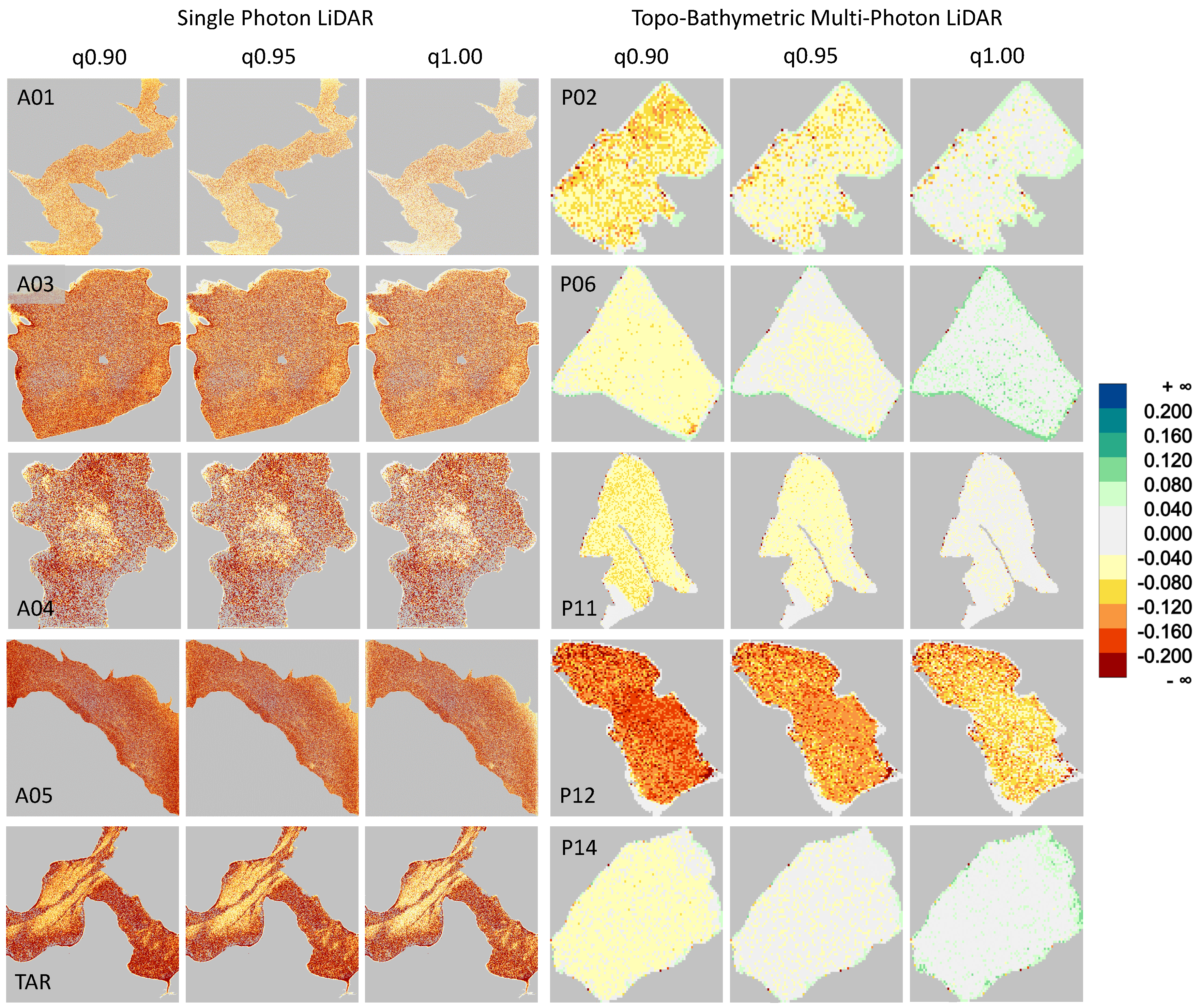
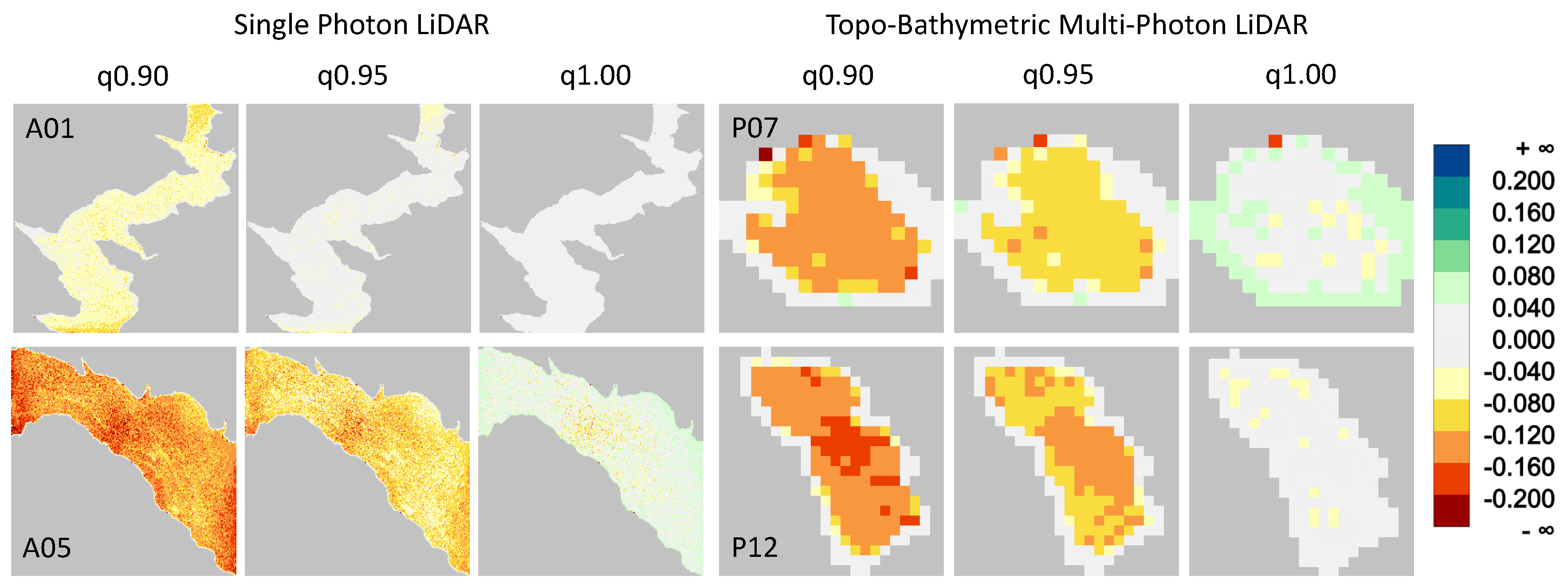
Quantitative assessment of the Single Photon LiDAR feasibility for high-resolution water surface mapping bases on multiple water surface raster models calculated for each test area with cell sizes of 1-, 2-, 5-, and 10 m resolution as described in Section 3.2 using the 50%/90%/95%/98%/99%/100% height quantile of all potential water points with a vertical distance from the reference water level of less than 50 cm. For the 2 m resolution rasters, Figure 9 depicts the deviations from the reference water level for investigation areas A01, A03, A04, A05, and TAR (Single Photon LiDAR) and P02, P06, P11, P12, and P14 (Topo-Bathymetric Multi-Photon LiDAR), respectively. The plot clearly reveals that the water level underestimation is generally less for the Multi-Photon LiDAR datasets as indicated by the whitish and yellowish color tones (0–8 cm) compared to the dominant red colors for the Single Photon LiDAR datasets (8–20 cm). The reflectance of the water surface and the topmost layer of the water column is, thus, not sufficient to reliably trigger water surface echoes even though the SPL100 features a detection probability of 95% for objects with 10% reflectivity. Again, as already stated in Section 4.2, a relation with turbidity is apparent, as water level underestimation is less for area A01 compared to the other evaluated Single Photon LiDAR datasets. The occasional gray dots in A03, A04, A05, and TAR indicate data voids, i.e., no water point was found in a 2 × 2 m cell in a 50 cm band below the water surface. Area A04 exhibits the highest number of data voids. The low water point density of this study area is also apparent from Figure 8.
Multi-Photon LiDAR performs better in this respect, with dominating white color tones for the max-height-in-cell estimator (i.e., 100% quantile) of P02, P06, P11, and P14. But still, accurate high-resolution water level results can not be achieved for all tested areas (cf. P12 in Figure 9). In general, the findings in this investigation are in line with [3], who concluded that water surface estimation based on discrete green-only 3D points requires appropriate spatial aggregation and the use of higher quantiles (e.g., 99%) for the histogram-based water level height estimation within each cell. The required aggregation level depends on the overall water point density, which is correlated with turbidity and water surface roughness. For selected areas, Figure 10 shows the deviations between the reference water level and water surface models with a cell size of 10 m. With this larger aggregation level, practically all tested water bodies show satisfactory conformance with the calculated reference water level. The Multi-Photon LiDAR test area P07 even shows a slight overestimation in the littoral area of about 5 cm. For Single Photon LiDAR, A01 matches the reference water surface nearly perfectly over the entire extent and A05, featuring a comparably low overall water point density, shows good agreement with this aggregation level as well.
To complete the picture, Table 4 lists the mean deviations from the reference water level for selected test areas based on the 99% quantile and different aggregation levels. It can be read from the last column of Table 4 that both Single- and Multi-Photon LiDAR yield water levels with a mean absolute deviation of less than 0.05 m for all tested water bodies by aggregating the points in 10 m raster cells. Some of the clear water areas (A03, A04, TAR, P07, P12) still show a moderate underestimation (e.g., TAR: −0.05 m) but, in turn, some areas even show water level overestimation using the 99% quantile estimator (P02, P04, P06, P14). As expected, the amount of under estimation generally increases with decreasing cell sizes. While many of the Topo-Bathymetric test areas (e.g., P05, P06, P11, P14) still feature moderate water level underestimation for the 1 m resolution (e.g. P14: −0.02 m), the water surface point density is generally too low for the Single Photon LiDAR test areas with a mean error ranging from −0.11 m (A01) to −0.21 m (A05). Furthermore, the mean deviation values reported in Table 4 once again underline that the green laser echoes show a considerable variation of subsurface penetration for the individual water bodies both for Single Photon LiDAR and Topo-Bathymetric Multi-Photon LiDAR.
5. Discussion
In this section, we discuss the results obtained from analyzing Single- and Multi-Photon LiDAR datasets (Section 4) in the context of the theoretical considerations concerning the interaction of green laser radiation with the medium water (Section 2.2). When comparing the available datasets on a general level, we conclude:
- Over land, the expected relation of global flight strip fitting precision and local measurement precision between Single Photon LiDAR (3 cm) and Multi-Photon LiDAR (1 cm) could be verified (cf. Table 3). The high Multi-Photon LiDAR precision can be attributed to the fact that about 250 photons are necessary for echo detection and range measurement, while the arrival of a few photons already trigger an echo in the Single Photon LiDAR case. The Easton SPL dataset, however, competes with Multi-Photon LiDAR concerning precision (both 1.3 cm). The Easton dataset features predominantly smooth and horizontal terrain (sealed roads, flat roofs, etc.). The precision of Single- and Multi-Photon full-waveform LiDAR was assessed in [46]. The authors reported that the superiority of Multi-Photon LiDAR w.r.t. precision is only observed in complex target situations (tilted surfaces, rough terrain, low object reflectance, grassy environments) while both technologies provide a local precision in the centimeter range for smooth horizontal targets. The specific study sites of the Navarra dataset, in turn, are mainly located in areas with undulating terrain (cf. Figure 3), which therefore exhibit a lower measurement precision. The reported measurement precision is considered a best-case case scenario for the achievable water surface height precision.
- Within the water area, Single Photon LiDAR yields a considerably lower last-echo point density compared to Topo-Bathymetric Multi-Photon LiDAR. In our experiment, we observe a density drop of 50% compared to the land area for Single Photon LiDAR. For Multi-Photon LiDAR, a point density drop is only observed for very clear water conditions. In both cases, we notice a correlation between turbidity and point density. This observation is backed up for the Multi-Photon LiDAR dataset by concurrent Secchi depth measurements. However, further experiments are needed to verify the relationship for Single Photon LiDAR.
- In general, the water level underestimation is less for Multi-Photon LiDAR and the respective (near) water surface point density is less for Single Photon LiDAR.
- Both data sources yield an acceptable agreement between local water surface heights and the reference water level by aggregating the near water surface points into 10 m raster cells and interpolating the surface height within a cell using a high quantile (e.g., 99%). The water surface underestimation remains below 4 cm in this case.
- For high-resolution water surface models with cell sizes of 1–2 m, the Single Photon LiDAR near water surface point density is too low to obtain a gapless model and Multi-Photon LiDAR outperforms Single Photon LiDAR in terms of precision.
The empirical findings resulting from processing the Single Photon LiDAR datasets of Navarra and Easton match the theoretical considerations outlined in Section 2.2 in general, and the photon counts calculated for different acquisition parameters and environmental conditions summarized in Table 2 in particular. We can state:
- For standard SPL100 flight mission parameters (Range: 4000 m, scan angle: 15), less than 2 photons are expected to be scattered back from the surface and the first 2 cm of the water column depending on the surface roughness (cf. Table 2a–c).
- For the same scenarios, a slight increase of the photon count from smooth to moderately rippled water surface conditions can be observed (r = 0.1 →0.3 ). The trend, however, reverses with a further increase of the surface roughness (r = 0.3 →0.5 ).
- In any case, the air–water interface reflection is dominating the contribution of volume backscattering from the first 2 cm of the water column. For the smooth water surface scenario (a), near surface volume backscattering only makes up 7% of the interface return (0.06 vs. 0.87 photons) and only 3% for the moderately rippled scenario (b).
- For smooth water surfaces, a reduction of the nominal incidence angle from 15 to 10 leads to approximately doubling the photon count, as can be seen from scenarios (a) and (d). This trend, however, is not observed for rough surfaces (cf. scenarios (b) and (e)), where the gain is only about 20%.
- Gradually lowering the measurement range leads to a constant increase of the received photon count from 2.2 photons for scenario (e) at a range of 4000 m to 40.9 photons for scenario (h) at a range of 1000 m.
These findings basically mean that Single Photon LiDAR based large-area water surface mapping is feasible, but specific flight mission parameters are necessary for reliable high-resolution water surface reconstruction. While the absolute values in Table 2 might not be entirely precise because the sensor internals are not officially available (e.g., optical and efficiency, etc.), we note that the empirical results presented in Section 4 support the reported numbers. Both the Navarra and Easton dataset were captured with the 15 scanning wedge from about 4000 m, and both datasets deliver occasional, but at least some points at the water surface. We conclude that the order of magnitude of the photon counts reported in Table 2 is principally correct. We especially expect that the relation of the reported photon counts corresponds to the parameter variation.
This leads us to the assumption that high-resolution water surface mapping is doable with Single Photon LiDAR when flying lower than 2000 m AGL and employing the 10 scanning wedge. Even with these restricted parameters, the swath width of a single SPL strip amounts to 705 m, which is about twice the width of a typical Topo-Bathymetric flight strip flown at 500 m with a constant off-nadir angle of 20. The expected higher spatial coverage constitutes a potential advantage of Single Photon LiDAR, but further experiments are required to validate the postulated feasibility for enabling both high-resolution and accurate water surface mapping.
Furthermore, it is stated that these findings were obtained from analyzing data of specific LiDAR sensors. While the general principles of laser light interaction with the medium water is common to any LiDAR (cf. Section 2.2), there are certainly differences in the detection strategy of Single- and Multi-Photon LiDAR in general and the individual instruments in particular. Especially the presented data processing results are representative for the respective sensors (SPL100, VQ-880-G) and the results might slightly deviate when using other Single- or Multi-Photon LiDAR sensors.
6. Conclusions and Outlook
In this article, we investigated the feasibility of Single Photon LiDAR for large-area water surface mapping. While literature already revealed that water surface mapping based on green laser light suffers from the potential penetration of the laser signal into the topmost layer of the water column [1,3,23], the specific research questions are if Single Photon LiDAR (i) consequently delivers a higher number of water surface echoes and (ii) is less effected by the well-known water surface-underestimation effect due the high receiver sensitivity.
We addressed the topic theoretically by recapturing the technological principles of Single- and Multi-Photon LiDAR and by reviewing laser light interaction with water. Based on a formulation of the laser-radar equation specialized for bathymetric applications [37,38] we calculated the expected number of photons arriving at the receiver for different flight mission parameters and environmental conditions.
In addition, we analyzed Single- and Multi-Photon LiDAR datasets of selected water bodies featuring a horizontal water level such as reservoirs and ponds. Data from the Spanish province Navarra and from Easton, MD, USA, captured with a Leica Geosystems SPL100 sensor were compared to Multi-Photon LiDAR data acquired with a RIEGL VQ-880-G Topo-Bathymetric laser scanner. Both instruments use green laser light ( = 532 nm) to measure objects on land (bare earth, vegetation, buildings, etc.) and water (surface and bottom). For both capturing techniques and for each water body the following processing steps were applied: flight block quality assessment including check of point density and strip registration precision, estimation of a reference water level, interpolation of different digital water surface raster models from all points with a water depth less than 50 cm in resolutions ranging from 1–10 m [3], and statistically analyzing the height deviations of the water surface models from the reference water level.
From processing and analyzing the available Single- and Multi-Photon LiDAR datasets we concluded: (i) water surface mapping is possible for both Single- and Multi-Photon Topo-Bathymetric LiDAR with an accuracy in the range of about 5 cm when aggregating the near water surface echoes into 5–10 m cells, (ii) the overall water point density is higher for Multi-Photon LiDAR, and (iii) high-resolution water surface mapping with grid sizes in the range of 1–2 m is unfeasible for Single Photon LiDAR when applying flight mission parameters optimized for topographic mapping. These findings coincide with the theoretical considerations, which fuel the expectation that Single Photon LiDAR based high-resolution water surface mapping is feasible with application specific flight mission parameters. Good results are expected when restricting the maximum flying altitude to less than 2000 m and using a 10 off-nadir scan angle instead of the standard 15 scanning wedge.
Future work on subject matters include the verification of the inferences formulated above in an upcoming project for mapping water surface heights of the Rhine River with the Leica SPL100 initiated by the Federal Institute of Hydrology (BfG, Koblenz, Germany). The findings of the presented article served as guideline for the flight planning. The aim of the project is to reconstruct tilted water surfaces in sub-decimeter accuracy as reference for the validation of hydrodynamic-numeric models. While accurate water surface reconstruction based on commercially available Single Photon LiDAR technology could not be confirmed for the standing water bodies analyzed in this study, better results are expected in the above-mentioned use case due to both the rippled structure of riverine water surfaces and the optimized flight mission parameters.
References
Author Contributions
G.M. designed the experiment, conducted data processing, and contributed the figures. B.J. was in charge of the theory section. Both authors jointly interpreted the data. The same applies to preparing, reviewing, and proofreading of the draft manuscript.
Funding
The presented investigation was conducted within the project “Bathymetry by Fusion of Airborne Laser Scanning and Multispectral Aerial Imagery” (SO 935/6-2) funded by the German Research Foundation (DFG).
Acknowledgments
The authors want to thank Roberto Pascual (Government of Navarra, Cartography Section) and Victor Garcia Morales (Tracasa) for providing the Leica SPL100 data of Navarra. Furthermore, we want to thank Leica Geosystems (Ron Roth) and RIEGL Laser Measurement Systems (Martin Pfennigbauer) for supplying the datasets of Easton and Pielach/Neubacher Au, respectively.
Conflicts of Interest
The authors declare no conflict of interest.
References
- Thomas, R.W.L.; Guenther, G.C. Water surface detection strategy for an airborne laser bathymeter. Proc. SPIE 1990, 1302, 1302–1315. [Google Scholar] [CrossRef]
- Rupnik, E.; Jansa, J.; Pfeifer, N. Sinusoidal Wave Estimation Using Photogrammetry and Short Video Sequences. Sensors 2015, 15, 30784–30809. [Google Scholar] [CrossRef] [Green Version]
- Mandlburger, G.; Pfennigbauer, M.; Pfeifer, N. Analyzing near water surface penetration in laser bathymetry—A case study at the River Pielach. ISPRS Annal. Photogr. Remote Sens. Spat. Inf. Sci. 2013, II-5/W2, 175–180. [Google Scholar] [CrossRef]
- Normandin, C.; Frappart, F.; Lubac, B.; Bélanger, S.; Marieu, V.; Blarel, F.; Robinet, A.; Guiastrennec-Faugas, L. Quantification of surface water volume changes in the Mackenzie Delta using satellite multi-mission data. Hydrol. Earth Syst. Sci. 2018, 22, 1543–1561. [Google Scholar] [CrossRef] [Green Version]
- Revilla-Romero, B.; Wanders, N.; Burek, P.; Salamon, P.; de Roo, A. Integrating remotely sensed surface water extent into continental scale hydrology. J. Hydrol. 2016, 543, 659–670. [Google Scholar] [CrossRef] [Green Version]
- Westaway, R.M.; Lane, S.N.; Hicks, D.M. Remote sensing of clear-water, shallow, gravel-bed rivers using digital photogrammetry. Photogramm. Eng. Remote Sens. 2001, 67, 1271–1281. [Google Scholar]
- Hodúl, M.; Bird, S.; Knudby, A.; Chénier, R. Satellite derived photogrammetric bathymetry. ISPRS J. Photogramm. Remote Sens. 2018, 142, 268–277. [Google Scholar] [CrossRef]
- Lyzenga, D.R.; Malinas, N.P.; Tanis, F.J. Multispectral bathymetry using a simple physically based algorithm. IEEE Trans. Geosci. Remote Sens. 2006, 44, 2251–2259. [Google Scholar] [CrossRef]
- Legleiter, C.J.; Dar, A.R.; Rick, L.L. Spectrally based remote sensing of river bathymetry. Earth Surf. Process. Landf. 2009, 34, 1039–1059. [Google Scholar] [CrossRef] [Green Version]
- Guenther, G.C.; Cunningham, A.G.; Laroque, P.E.; Reid, D.J. Meeting the accuracy challenge in airborne lidar bathymetry. In Proceedings of the 20th EARSeL Symposium: Workshop on Lidar Remote Sensing of Land and Sea, Dresdejn, Germany, 16–17 June 2000. [Google Scholar]
- Forfinski-Sarkozi, N.A.; Parrish, C.E. Analysis of MABEL Bathymetry in Keweenaw Bay and Implications for ICESat-2 ATLAS. Remote Sens. 2016, 8, 772. [Google Scholar] [CrossRef]
- Mandlburger, G. A Review of Airborne Laser Bathymetry Sensors. In Proceedings of the 5th IAHR EUROPE CONGRESS—New challenges in hydraulic research and engineering, Trento, Italy, 13–14 June 2018; pp. 41–42. [Google Scholar]
- Höfle, B.; Vetter, M.; Pfeifer, N.; Mandlburger, G.; Stötter, J. Water surface mapping from airborne laser scanning using signal intensity and elevation data. Earth Surf. Process. Landf. 2009, 34, 1635–1649. [Google Scholar] [CrossRef]
- Pekel, J.F.; Cottam, A.; Gorelick, N.; Belward, A.S. High-resolution mapping of global surface water and its long-term changes. Nature 2018, 540, 418–422. [Google Scholar] [CrossRef]
- Yang, F.; Su, D.; Ma, Y.; Feng, C.; Yang, A.; Wang, M. Refraction Correction of Airborne LiDAR Bathymetry Based on Sea Surface Profile and Ray Tracing. IEEE Trans. Geosci. Remote Sens. 2017, 55, 6141–6149. [Google Scholar] [CrossRef]
- Westfeld, P.; Maas, H.G.; Richter, K.; Weiß, R. Analysis and correction of ocean wave pattern induced systematic coordinate errors in airborne LiDAR bathymetry. ISPRS J. Photogramm. Remote Sens. 2017, 128, 314–325. [Google Scholar] [CrossRef]
- Mandlburger, G. Interaction of Laser Pulses with the Water Surface—Theoretical Aspects and Experimental Results. Allg. Vermess.-Nachrichten 2017, 124, 343–352. [Google Scholar]
- Stoker, J.M.; Abdullah, Q.A.; Nayegandhi, A.; Winehouse, J. Evaluation of Single Photon and Geiger Mode Lidar for the 3D Elevation Program. Remote Sens. 2016, 8, 767. [Google Scholar] [CrossRef]
- Ullrich, A.; Pfennigbauer, M. Linear LIDAR versus Geiger-mode LIDAR: impact on data properties and data quality. Proc. SPIE 2016, 9832, 983204–983217. [Google Scholar] [CrossRef]
- Ullrich, A.; Pfennigbauer, M. Noisy lidar point clouds: impact on information extraction in high-precision lidar surveying. Proc. SPIE 2018, 10636, 106360M-1–106360M-6. [Google Scholar] [CrossRef]
- Degnan, J.J. Scanning, Multibeam, Single Photon Lidars for Rapid, Large Scale, High Resolution, Topographic and Bathymetric Mapping. Remote Sens. 2016, 8, 958. [Google Scholar] [CrossRef]
- Shan, J.; Toth, C.K. (Eds.) Topographic Laser Ranging and Scanning: Principles and Processing, 2nd ed.; CRC Press: Boca Raton, FL, USA, 2018; p. 638. [Google Scholar]
- Zhao, J.; Zhao, X.; Zhang, H.; Zhou, F. Shallow Water Measurements Using a Single Green Laser Corrected by Building a Near Water Surface Penetration Model. Remote Sens. 2017, 9, 426. [Google Scholar] [CrossRef]
- Leica. SPL100 Single Photon LiDAR Sensor Data Sheet; Leica Geosystems: Heerbrugg, Switzerland, 2019. [Google Scholar]
- Riegl. VQ-880-G Topo-Bathymetric LiDAR Sensor Data Sheet; Riegl Laser Measurement Systems: Horn, Austria, 2019. [Google Scholar]
- Jutzi, B. Less Photons for More LiDAR? A Review from Multi-Photon Detection to Single Photon Detection. In Proceedings of the 56th Photogrammetric Week (PhoWo), Stuttgart, Germany, 17 March 2017. [Google Scholar]
- Pfennigbauer, M.; Ullrich, A. Improving quality of laser scanning data acquisition through calibrated amplitude and pulse deviation measurement. Proc. SPIE 2010, 7684, 76841F-1–76841F-10. [Google Scholar] [CrossRef]
- Gys, T. Micro-channel plates and vacuum detectors. Nucl. Inst. Method. Phys. Res. Sect. A Accel. Spectrom. Detect. Assoc. Equip. 2015, 787, 254–260. [Google Scholar] [CrossRef] [Green Version]
- Agishev, R.; Comerón, A.; Bach, J.; Rodriguez, A.; Sicard, M.; Riu, J.; Royo, S. Lidar with SiPM: Some capabilities and limitations in real environment. Opt. Laser Technol. 2013, 49, 86–90. [Google Scholar] [CrossRef]
- Dautet, H.; Deschamps, P.; Dion, B.; MacGregor, A.D.; MacSween, D.; McIntyre, R.J.; Trottier, C.; Webb, P.P. Photon counting techniques with silicon avalanche photodiodes. Appl. Opt. 1993, 32, 3894–3900. [Google Scholar] [CrossRef]
- McCarthy, A.; Collins, R.J.; Krichel, N.J.; Fernández, V.; Wallace, A.M.; Buller, G.S. Long-range time-of-flight scanning sensor based on high-speed time-correlated single photon counting. Appl. Opt. 2009, 48, 6241–6251. [Google Scholar] [CrossRef]
- Jutzi, B.; Stilla, U. Analysis of laser pulses for gaining surface features of urban objects. In Proceedings of the 2nd GRSS/ISPRS Joint Workshop on Remote Sensing and Data Fusion over Urban Areas, Berlin, Germany, 22–23 May 2003; IEEE: Piscataway, NJ, USA, 2003; pp. 13–17. [Google Scholar]
- Jutzi, B.; Stilla, U. Waveform processing of laser pulses for reconstruction of surfaces in urban areas. In ISPRS Joint Conference 3rd International Symposium Remote Sensing and Data Fusion over Urban Areas (URBAN 2005), Proceedings of the 5th International Symposium Remote Sensing of Urban Areas (URS 2005), Tempe, AR, USA, 14–16 March 2005; ISPRS: Hannover, Germany; p. 6.
- Wagner, W. Radiometric calibration of small-footprint full-waveform airborne laser scanner measurements: Basic physical concepts. ISPRS J. Photogramm. Remote Sens. 2010, 65, 505–513. [Google Scholar] [CrossRef]
- Höfle, B.; Pfeifer, N. Correction of laser scanning intensity data: Data and model-driven approaches. ISPRS J. Photogramm. Remote Sens. 2007, 62, 415–433. [Google Scholar] [CrossRef]
- Jelalian, A.V. Laser Radar Systems; Artech House Radar Library: London, UK, 1992. [Google Scholar]
- Abdallah, H.; Baghdadi, N.; Bailly, J.S.; Pastol, Y.; Fabre, F. Wa-LiD: A New LiDAR Simulator for Waters. IEEE Geosci. Remote Sensing Lett. 2012, 9, 744–748. [Google Scholar] [CrossRef] [Green Version]
- Tulldahl, H.M.; Steinvall, K.O. Simulation of sea surface wave influence on small target detection with airborne laser depth sounding. Appl. Opt. 2004, 43, 2462–2483. [Google Scholar] [CrossRef]
- Cook, R.L.; Torrance, K.E. A Reflectance Model for Computer Graphics. ACM Trans. Graph. 1982, 1, 7–24. [Google Scholar] [CrossRef]
- Beckmann, P.; Spizzichino, A. The Scattering of Electromagnetic Waves from Rough Surfaces; Pergamon Press: Oxford, UK, 1963; p. 512. [Google Scholar]
- Richter, K.; Maas, H.G.; Westfeld, P.; Weiß, R. An Approach to Determining Turbidity and Correcting for Signal Attenuation in Airborne Lidar Bathymetry. PFG J. Photogramm. Remote Sens. Geoinf. Sci. 2017, 85, 31–40. [Google Scholar] [CrossRef]
- Mandlburger, G.; Hauer, C.; Wieser, M.; Pfeifer, N. Topo-bathymetric LiDAR for monitoring river morphodynamics and instream habitats—A case study at the Pielach River. Remote Sens. 2015, 7, 6160–6195. [Google Scholar] [CrossRef]
- Pfeifer, N.; Mandlburger, G.; Otepka, J.; Karel, W. OPALS—A framework for Airborne Laser Scanning data analysis. Comput. Environ. Urban Syst. 2014, 45, 125–136. [Google Scholar] [CrossRef]
- Otepka, J.; Mandlburger, G.; Karel, W. The OPALS data manager—Efficient data management for processing large airborne laser scanning projects. ISPRS Annal. Photogramm. Remote Sens. Spat. Inf. Sci. 2012, I-3, 153–159. [Google Scholar] [CrossRef]
- Ressl, C.; Kager, H.; Mandlburger, G. Quality checking of als projects using statistics of strip differences. Int. Arch. Photogramm. Remote Sens. 2008, XXXVII, 253–260. [Google Scholar]
- Mandlburger, G.; Lehner, H.; Pfeifer, N. A Comparison of Single Photon and Full Waveform LiDAR. ISPRS Annal. Photogramm. Remote Sens. Spat. Inf. Sci. 2019, II. in press. [Google Scholar]
- Frazier, P.S.; Page, K.J. Water body detection and delineation with Landsat TM data. PERS Photogramm. Eng. Remote Sens. 2000, 66, 1461–1467. [Google Scholar]
Figure 1.
Typical optical receiver scenario for conventional Multi-Photon LiDAR and recent Single Photon LiDAR; (a) single optical receiver; (b) array showing 10 × 10 beamlet projections, where each beamlet projection illuminates photosensitive sub-arrays with numerous detector elements (pixelated array detector). The dashed circles indicate different possible relations of footprint size vs. receiver’s iFOV.

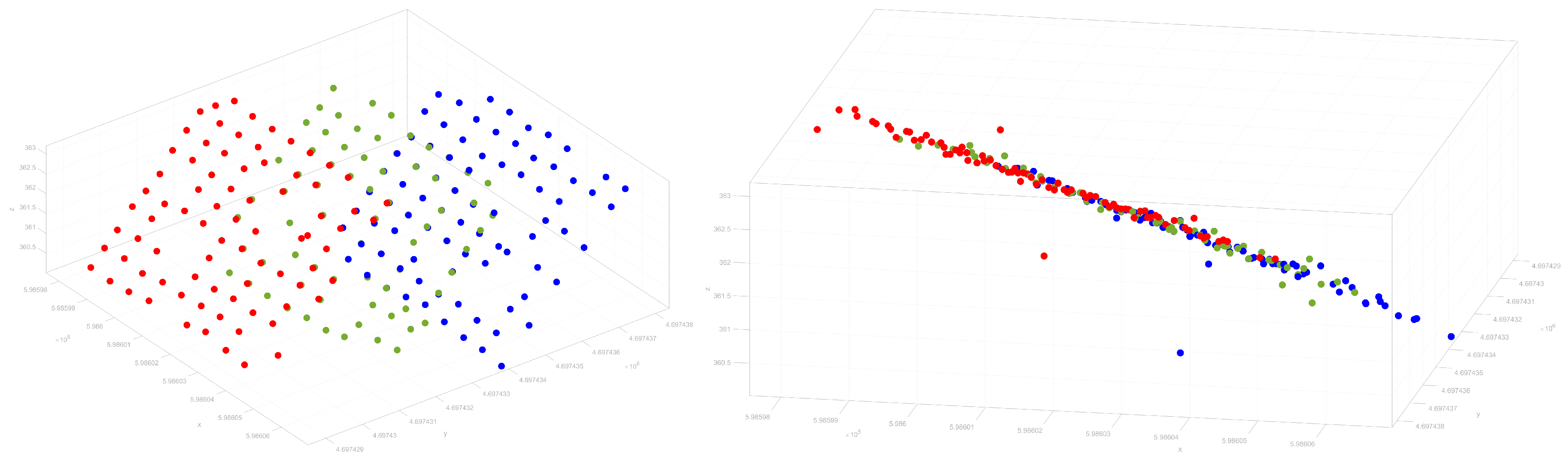
Figure 2.
Three consecutive Single Photon LiDAR point measurements (red, green, blue) indicating the regular scan grid caused by the 100 beamlets per laser pulse; (left) oblique 3D view of the point cloud, (right) profile view of the same point cloud.
Figure 2.
Three consecutive Single Photon LiDAR point measurements (red, green, blue) indicating the regular scan grid caused by the 100 beamlets per laser pulse; (left) oblique 3D view of the point cloud, (right) profile view of the same point cloud.

Figure 3.
Single Photon LiDAR area Navarra, Northern Spain; (a) foreground: base map of Navarra, background: OpenStreetMap, yellow boxes: selected reservoirs (A01-05), coordinate frame: WGS84/UTM 30N, units = meters; (b) overview map of Spain; (c) detailed terrain relief maps of reservoir areas A01, A03-05; coordinate grids: 1 km.

Figure 4.
Single Photon LiDAR area Easton, MD, USA; (a) shaded relief map of flight strip 3 on top of Google Bing orthophoto, coordinate reference frame: WGS 84, UTM 18N, ellipsoid heights, units = meters; center: analysis area, combination of shaded relief and color-coded height map; (b) overview map of the USA (source: USGS), red circle: location of study area.

Figure 5.
Topo-Bathymetric LiDAR area Neubacher Au, Pielach River, Austria; (a) overview map of Austria, red circle: location of the study area; (b) Digital Surface Model of Neubacher Au flood plain with groundwater supplied ponds (blue polygons), combination of shaded relief and color-coded height map, coordinate reference frame: ETRS89/UTM 33N, ellipsoid heights, units = meters.

Figure 6.
Perspective views of 3D point clouds; (a) Single Photon LiDAR (Navarra), (b) Single Photon LiDAR (Easton), (c) Multi-Photon LiDAR (Neubacher Au); size of displayed areas: 75 m × 50 m.
Figure 6.
Perspective views of 3D point clouds; (a) Single Photon LiDAR (Navarra), (b) Single Photon LiDAR (Easton), (c) Multi-Photon LiDAR (Neubacher Au); size of displayed areas: 75 m × 50 m.

Figure 7.
Color-coded point density maps [points/m] for Single Photon LiDAR (a,b) and Multi-Photon LiDAR (c).
Figure 7.
Color-coded point density maps [points/m] for Single Photon LiDAR (a,b) and Multi-Photon LiDAR (c).

Figure 8.
Selected vertical sections; Left column: Single Photon LiDAR (Navarra: A01–A05, Easton: TAR); Right column: Topo-Bathymetric Multi-Photon LiDAR; blue: water candidate points, orange: points on dry land, red line: estimated water level. Section width: 30 m, section depth: 3 m, height range: 2 m.

Figure 9.
Deviations between reference water level and 2 m digital water surface model grids calculated for selected Single- and Multi-Photon LiDAR water bodies and height quantiles.
Figure 9.
Deviations between reference water level and 2 m digital water surface model grids calculated for selected Single- and Multi-Photon LiDAR water bodies and height quantiles.

Figure 10.
Deviations between reference water level and 10 m digital water surface model grids calculated for selected Single- and Multi-Photon LiDAR water bodies and height quantiles.
Figure 10.
Deviations between reference water level and 10 m digital water surface model grids calculated for selected Single- and Multi-Photon LiDAR water bodies and height quantiles.


Table 1.
Specifications for Single Photon LiDAR, Multi-Photon LiDAR, and Topo-Bathymetric LiDAR. For generalization purpose a standard combination of specifications from various companies is provided for conventional Multi-Photon LiDAR.
Table 1.
Specifications for Single Photon LiDAR, Multi-Photon LiDAR, and Topo-Bathymetric LiDAR. For generalization purpose a standard combination of specifications from various companies is provided for conventional Multi-Photon LiDAR.
| Single Photon LiDAR | Multi-Photon LiDAR | Topo-Bathym. LiDAR | |
|---|---|---|---|
| Type | Leica/Hexagon SPL100 | various | RIEGL VQ-880-G |
| Laser wavelength | 532 nm | 532/1064/1550 nm | 532 nm |
| Laser pulse width (FWHM) | 400 ps | 1-5 ns | 1.6 ns |
| Beam divergence @ 1/e2 | ∼0.08 mrad/beamlet | 0.25–1 mrad | 0.7–1 mrad |
| Field of View (FoV) | 20, 30, 40 or 60 | ≤72 | 40 |
| Detector elements | hundreds | 1–2 PIN/APD | 1–2 APD |
| Intensity measurement | available | available, up to 16 bit | available, up to 16 bit |
| Min. # for object detection | 1 photon | 250–1000 photons | 250 photons |
| Instantaneous FoV (iFoV) | N/A | 0.25–1 mrad | 0.7–1 mrad |
| Jitter/ranging precision | 50–100 ps / 0.75–1.5 cm | 50–500 ps/0.75–7.5 cm | N/A / 2.5 cm |
| Dead time/recovery time | 1.6 ns | N/A | N/A |
| Pulse repetition rate (PRR) | 60 kHz | ≤1000 kHz | 550 kHz |
| Max. flying altitude (AGL) | ≤4500 m | ≤5000 m | ≤2200 m/Bathy 600 m |
| Areal coverage @ 8 pts/m2 | ≤2000 km2/h | ≤450 km2/h | ≤150 km2/h |
Table 2.
Estimated photon count for representative data acquisition scenarios and surface conditions.
Table 2.
Estimated photon count for representative data acquisition scenarios and surface conditions.
| Scenario | Description | R | r | |||||
|---|---|---|---|---|---|---|---|---|
| a | high altitude, medium angle, smooth | 4000 m | 15 | 0.1 | 0.03 | 0.87 | 0.06 | 0.93 |
| b | high altitude, medium angle, rippled | 4000 m | 15 | 0.3 | 0.07 | 1.80 | 0.06 | 1.85 |
| c | high altitude, medium angle, rough | 4000 m | 15 | 0.5 | 0.05 | 1.42 | 0.06 | 1.48 |
| d | high altitude, small angle, smooth | 4000 m | 10 | 0.1 | 0.06 | 1.60 | 0.06 | 1.66 |
| e | high altitude, small angle, rippled | 4000 m | 10 | 0.3 | 0.08 | 2.17 | 0.05 | 2.23 |
| f | medium altitude, small angle, rippled | 3000 m | 10 | 0.3 | 0.08 | 4.05 | 0.10 | 4.15 |
| g | low altitude, small angle, rippled | 2000 m | 10 | 0.3 | 0.08 | 9.53 | 0.24 | 9.77 |
| h | very low altitude, small angle, rippled | 1000 m | 10 | 0.3 | 0.08 | 39.93 | 0.99 | 40.92 |
Table 3.
Flight mission and qualitycontrol parameters for Single Photon LiDAR (SPL: Navarra, Spain and Easton, MD, USA) and Multi-Photon LiDAR (MPL: Neubacher Au, Austria).
Table 3.
Flight mission and qualitycontrol parameters for Single Photon LiDAR (SPL: Navarra, Spain and Easton, MD, USA) and Multi-Photon LiDAR (MPL: Neubacher Au, Austria).
| Unit | SPL-Navarra | SPL-Easton | MPL | |
|---|---|---|---|---|
| Flying velocity | [m/s] | 90 | 70 | 55 |
| Flying altitude | [m] | 4200 | 3750 | 650 |
| Pulse repetition rate | [kHz] | 60 | 50 | 550 |
| Effective scan rate | [kHz] | 6000 | 5000 | 550 |
| Strip swath width | [cm] | 2260 | 2000 | 480 |
| Footprint diameter | [cm] | 35 | 30 | 70 |
| DEM precision/roughness | [cm] | 3.0 | 1.3 | 1.3 |
| Scan registration precision | [cm] | 3.9 | 3.0 | 1.2 |
| Strip point density (land) | [cm] | 14.5 | 12.0 | 14.0 |
| Strip point density (water) | [cm] | 7.0 | 4.3 | 12.5 |
| Scan pattern | circular | circular | circular | |
| Total FOV | [] | 30 | 30 | 40 |
Table 4.
Mean deviations [m] of different digital water surface models from the reference water level for the 99% quantile.
Table 4.
Mean deviations [m] of different digital water surface models from the reference water level for the 99% quantile.
| 1.0 m | 2.0 m | 5.0 m | 10.0 m | |
|---|---|---|---|---|
| A01 | −0.11 | −0.06 | 0.00 | 0.02 |
| A03 | −0.16 | −0.11 | −0.05 | −0.02 |
| A04 | −0.17 | −0.17 | −0.09 | −0.03 |
| A05 | −0.21 | −0.16 | −0.06 | −0.03 |
| TAR | −0.19 | −0.16 | −0.08 | −0.05 |
| P02 | −0.06 | −0.02 | 0.01 | 0.02 |
| P04 | −0.05 | −0.02 | −0.00 | 0.01 |
| P05 | −0.04 | −0.02 | −0.01 | 0.00 |
| P06 | −0.02 | 0.00 | 0.01 | 0.02 |
| P07 | −0.15 | −0.09 | −0.06 | −0.03 |
| P08 | −0.08 | −0.04 | −0.01 | −0.02 |
| P11 | −0.05 | −0.03 | −0.02 | −0.01 |
| P12 | −0.15 | −0.10 | −0.06 | −0.04 |
| P14 | −0.02 | −0.01 | 0.00 | 0.01 |
© 2019 by the authors. Licensee MDPI, Basel, Switzerland. This article is an open access article distributed under the terms and conditions of the Creative Commons Attribution (CC BY) license (http://creativecommons.org/licenses/by/4.0/).
Share and Cite
MDPI and ACS Style
Mandlburger, G.; Jutzi, B. On the Feasibility of Water Surface Mapping with Single Photon LiDAR. ISPRS Int. J. Geo-Inf. 2019, 8, 188. https://0-doi-org.brum.beds.ac.uk/10.3390/ijgi8040188
AMA Style
Mandlburger G, Jutzi B. On the Feasibility of Water Surface Mapping with Single Photon LiDAR. ISPRS International Journal of Geo-Information. 2019; 8(4):188. https://0-doi-org.brum.beds.ac.uk/10.3390/ijgi8040188
Chicago/Turabian StyleMandlburger, Gottfried, and Boris Jutzi. 2019. "On the Feasibility of Water Surface Mapping with Single Photon LiDAR" ISPRS International Journal of Geo-Information 8, no. 4: 188. https://0-doi-org.brum.beds.ac.uk/10.3390/ijgi8040188
Note that from the first issue of 2016, this journal uses article numbers instead of page numbers. See further details here.