Could Crime Risk Be Propagated across Crime Types?


1
College of Civil Engineering, Nanjing Forestry University, Nanjing 210037, China
2
National Engineering Research Center of Biomaterials, Nanjing Forestry University, Nanjing 210037, China
3
Key Laboratory of Virtual Geographic Environment, Ministry of Education, Nanjing Normal University, Nanjing 210046, China
4
Jiangsu Center for Collaborative Innovation in Geographical Information Resource Development and Application, Nanjing Normal University, Nanjing 210046, China
*
Author to whom correspondence should be addressed.
ISPRS Int. J. Geo-Inf. 2019, 8(5), 203; https://0-doi-org.brum.beds.ac.uk/10.3390/ijgi8050203
Submission received: 23 March 2019
/
Revised: 26 April 2019
/
Accepted: 2 May 2019
/
Published: 4 May 2019
(This article belongs to the Special Issue Urban Crime Mapping and Analysis Using GIS)
Abstract
:It has long been acknowledged that crimes of the same type tend to be committed at the same location or proximity in a short period. However, the investigation of whether this phenomenon exists across crime types remains limited. The spatial-temporal clustered patterns for two types of crimes in public areas (pocket-picking and vehicle/motor vehicle theft) are separately examined. Compared with existing research, this study contributes to current research from three aspects: (1) The repeat and near-repeat phenomenon exists in two types of crimes in a large Chinese city. (2) A significant spatial-temporal interaction between pocket-picking and vehicle/motor vehicle theft exists within a range of 100 m. Some cross-crime type interactions seem to have a stronger ability of prediction than does single-crime type interaction. (3) A risk-avoiding activity is identified after spatial-temporal hotspots of another crime type. The spatial extent with increased risk is limited to a certain distance from the previous hotspots. The experimental results are analyzed and interpreted with current criminology theories.
1. Introduction
As a branch of environmental criminology research, crime pattern research has attracted the attention of many researchers due to its potential in helping people understand the dimensions of risk and optimize the efficiency of crime reduction effort [1,2]. As an important discovery in crime pattern research, the repeat and near-repeat (RNR) phenomenon provides insight into a more precise understanding of crime distribution. The RNR phenomenon suggests that crimes are spatially and temporally correlated. The information can be transferred from one crime to another crime within a certain distance and a certain time period [3,4,5]. According to the crime types, research of RNR can be separated into two categories: RNR within a single crime type and RNR across different crime types.
RNR is primarily examined within a single crime type. Bowers and Johnson suggested that a recorded burglary victim, as a starting point in RNR, is a variant of risk predictors for burglaries [3]. The offenders would become more familiar with the modus operandi on a victimized place or object and, subsequently, repeat similar offense types in nearby households. Street robbery and gun violence share similar RNR patterns according to other research [4,6].
Compared with classic research on the risk after each crime, other research has considered spatial-temporal hotspots with RNR calculation [7,8,9]. Hotspots can be classified into spatial hotspots, temporal hotspots, and spatial-temporal hotspots [7]. In this study, a ‘spatial-temporal hotspot’ is referred to as a ‘hotspot.’ The information dissemination mechanism among offenders exists among crime types.
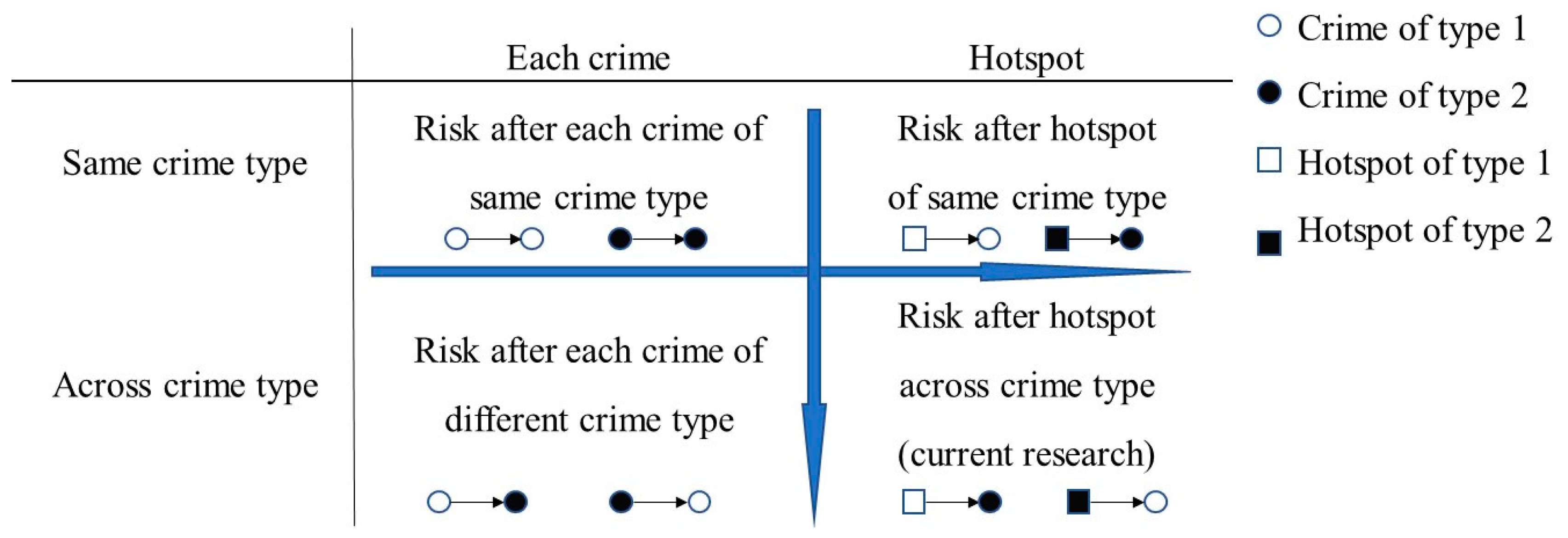
Compared with the distinct relationship among the same type crimes, the research of correlations among different types of crimes need to be investigated. Johnson et al. attempted to detect the existence of RNR patterns among different crime types [10,11,12]. Using burglary and theft from motor bicycle data, the RNR pattern was investigated. The results indicate a lack of support for this hypothesis. However, further research is “clearly warranted to see if such patterns exist” among other crime types [10]. The observed phenomenon contributed additional knowledge of crime distribution to research and is expected to benefit the patrol efficacy of practitioners. Existing research provides a new opportunity to gain insight into the impact of hotspots on the crime rate of different types (Figure 1).
In this paper, we will examine the spatial-temporal pattern of two crime types: Pocket-picking (PP) and vehicle, motor vehicle theft (VMVT) using crime data collected by the police department in a large Chinese city. First, we will review previous research and outline the theoretical framework of the tested questions. We will present the RNR patterns after hotspots with different crime types after the RNR test within and across the two listed crime types. This research will determine whether risk can be transferred within crime type. In the third part, we will consider the risk undulation from the results and determine if risk can be transferred among crime types by concluding the crime contagion pattern. This analysis can help optimize crime prevention strategies and improve patrol efficacy.
PP is defined as the theft of property carried by somebody else on ‘public area’ or ‘public transports.’ ‘Public area’ and “carried by somebody else’ are two core components of the definition of VMVT. Corresponding to the definition of VMVT, the VMVT can be defined as the theft of a bicycle, motorcycle, or car that cannot carried by somebody else in a ‘public area.’
2. Literature Review
The crime propagation phenomena, which is known as RNR, have attracted a substantial amount of attention in criminological research. Two hypotheses account for the RNR phenomenon: The boost hypothesis and the flag hypothesis. The boost account suggests that short-run space-time clustering is boosted by the initial crime [13,14]. Previous offenders will transfer information or experience of the victims to future offenders. Future offenders return to the targeted victims and commit another crime by experience. The following crimes seem to be ‘boosted’ by the initial crime. The notion that most clustered crimes are committed by serial offenders or gang members strongly supports the ‘boost’ hypothesis [10,15,16]. The flag account argues that most repeatedly victimized places (or locations) are flagged by opportunistic offenders due to their special properties. Offenders are assumed to be attracted by the targets and to commit similar crimes on the same (or nearby) victims in a period of time [13]. Both boost accounts and flag accounts have been employed to interpret RNR victimizations.
Many crime theories can account for the RNR phenomenon. Crime pattern theory recognizes place as a core factor that affects the crime distribution [17]. For example, places with mixed land use (e.g., commercial and civic institutional recreation land use) are usually subjected to high risk because they are comparatively more attractive to offenders than other people [18]. By this theory, potential offenders that are attracted by particular objects (or locations) are assumed to repeatedly commit similar crimes or inform other group members to commit similar crimes by sharing the learned experience/modus operandi, such as what boost account is hypothesized. Routine activity theory argues that people’s routine activity determines crime distribution [19]. In this theory, potential offenders repeat daily routine activities and commit a crime until sufficient conditions (copresented unprotected target and motivated offenders) are fulfilled [20]. From the viewpoint of routine activity theory, the RNR is derived from people’s routine activities. For many of the offenders, committing crimes is a part of routine activities. Vulnerable objects are more likely to satisfy the conditions and are easily violated by potential offenders. In this case, vulnerable objects have roles as information transmitters which can distribute risk information to similar potential offenders. All aforementioned theories provide explanations of RNR and accept that the experience of victimization (modus operandi and object’s characteristics) can be spatially and temporally transformed within the same crime type.
Though the RNR phenomenon informs of the increased risk after each crime victimization, the phenomena of crime spatiotemporal displacement focus on the decreased crime risk after hotspots, according to Nakaya’s and Zengli’s research [8,9]. According to their research, the risk will not increase immediately after hotspots but will immediately decrease in the proximity area and then “return” to the same locations after a short period. The phenomena of crime transformation can be interpreted as a risk-avoiding activity of offenders. When the crime risk within an area is excessive, the potential offenders can feel the increased risk and then displace it to other places or other crime types. When the risk disappeared, potential offenders may return and search for more crime opportunities at the same locations. In the ‘return’ activity, potential offenders are attracted by objects after the risk is decreased or even disappears [18]. In this case, the ‘avoiding’ and ‘return’ activities indicate that the risk status within hotspots can be ‘felt’ by the potential offenders. The existence of experience transformation between two crimes is further confirmed. However, similar to RNR research, crime displacement research remains within a single crime type.
Beyond single crime type research, crimes of different types are also hypothesized to be related based on several common facts. For example, some breaking and entering offenses may change to rape after the male potential offender sees a single female in a burglary [21]. A VMVT may change to robbery if the offender was felt/caught at the moment of stealing [22]. Other hypotheses support the existence of a relationship between two different types. For example, some offenders may displace their modus operandi if they determine that their current modus operandi is outdated or at high risk of being caught by a policeman. Several kinds of displacement exist [23]. The change in the modus operandi is a classic displacement type. Offenders can displace to other crime types after they determine that a targeted area (or object) is subject to high risk. However, the current literature on the relationship between two crime types yields negative results. Burglary and theft from motor vehicle (TFMV) are two significantly different crime types. Most burglaries occur in victims’ homes, while TFMV primarily (37 percent) occur in public areas, such as streets and parking lots [11]. Furthermore, many of the techniques (e.g., car opening) associated with auto theft are distinct to those of burglary [11,12]. It is difficult for an offender to easily duplicate the technique or experience learned in a burglary to a TFMV and vice versa. This difficulty can cause a lack of information exchange between the offenders of two crimes and objectively lead to the non-existence of the RNR pattern between two crimes. Further research about the relationship between two distinct crime types remains vague.
In current research, PP and VMVT are selected as research objects. VMVT victimizations are spatially clustered according to the literature [24,25,26,27]. Obviously, the parking lots and garages where many VMVT are situated with little guardianship are usually identified as VMVT hot areas [24,28,29]. Further research indicates that a large proportion of VMVTs occur at residential locations [30]. Research about PP crime indicates that PPs are concentrated in some special places [31,32,33,34]. A great number of PPs occurs at bus stops [31] and tourist attractions [32]. In short, these two crime types have been investigated and have been reportedly clustered in space. However, further research about the relationship between distinct crime types is still vague.
Inspired by the current gap, three questions are proposed in this study:
Question 1: Are the PPs and VMVTs spatially and temporally correlated within one crime type in a large Chinese city?
Many empirical and experimental studies have verified the existence of the RNR phenomenon with burglary data of Chinese cities [8,15,35,36,37]. However, this research may be the first attempt to investigate the existence of the RNR phenomenon among PP and VMVT records in a large Chinese city. This experiment can determine whether crimes are spatially and temporally correlated within each crime type.
Question 2: Does the interaction effect exist among different crime types?
Though current research has denied the spatial-temporal relationship between two crime types, further research about the RNR relationship among other crime types is warranted [10]. The results of this experiment will heighten our understanding of the relationship among crime types.
Question 3: If hypothesis 2 is confirmed, then another hypothesis will be proposed; that is, whether or not a significant undulation of crime risk occurs after hotspots with the heterogenous crime type.
Though this research has acknowledged that hotspots can affect the crime risk within the proximity area for a period within the same crime type, the impact on other crime types remains to be investigated. Based on this research, two distinct risk statuses exist immediately after hotspots of another crime type: Increased risk and decreased risk. After a hotspot, the potential offenders are hypothesized to change their modus operandi and even commit other kinds of crimes. The crime risk of another crime type will increase immediately after hotspots. Correspondingly, the high crime risk caused by the hotspots can also be hypothesized to transform the risk information to other crime types offenders and deter them from this area for a period. Additional experiments are needed to determine which of these hypotheses is correct.
3. Methodology
3.1. Knox Test
The Knox test was originally developed to detect spatial-temporal clusters of disease events in epidemiology [38]. In recent decades, this statistical method has been extensively adopted to identify crime hotspots in the criminology research area [39]. Theoretically, the Knox test examines if the event pairs with a specified spatial-temporal range exceed the expected number in a random simulation. In this test, the space-time distances between two event pairs will be calculated and then counted in a predefined matrix. Space and time bandwidths of the matrix are usually defined as 100 m × 7 days or 200 m × 14 days [40]. The value of each cell represents the number of event pairs with a certain space-time distance. Subsequently, a Monte Carlo simulation will be performed to build a group of numbers for each cell in the matrix. The simulated matrix will be used to determine the significance level and the expectation value of each cell value in the first matrix. The near-repeat matrix will be calculated with the first matrix divided by the expectation matrix determined by the Monte Carlo simulation. The confidence level of every unit will be determined by the number of observed units that exceed the expected unit values for all simulations. The Monte Carlo simulation will be generated by 999 permutations. The risk level within a specific space-time band is the ratio of the observed number of incidents and the average number from the simulations. A larger ratio indicates a higher risk level in the space-time band. The significance level for each cell value is determined by calculating the number of times of the observed event pairs exceeds the mean of the expected distribution. A small value means a high significance level. For instance, when the number of observed event pairs is greater than 996 simulated counts, the significance level is 1–996/(999) = 0.004.
The Knox test is a risk detector by a comparison of the distribution of events against a random distribution. The near-repeat matrix generated in the Knox test indicates the possibility of another event. According to the criminology research, the spatially and temporally close crime event pairs are more correlated than other pairs [3,15]. Correspondingly, the cell value with a short space-time distance in the near repeat matrix will be significantly higher than others cell values.
3.2. Knox Test for Interaction between Two Crime Types
To examine the interaction effect between crimes of two types, a modified Knox test was proposed by Johnson et al. [10]. In this method, the space-time distance between two crime types was calculated to replace the distance between the same crime types. In contrast to the distance calculated in the same crime type based on the Knox test, the modified Knox test will only calculate the distance with the early events as starting points. Thus, a contingency table, in which each cell represents the count of distances between two types of crimes, will be computed. A Monte Carlo simulation will be employed again to generate the expected distribution. Note that the Monte Carlo simulation will be used to simulate subsequent events in crime event pairs. The expected distribution will be used to determine the expected value of each cell and the significance of the cell values in the near-repeat matrix.
3.3. Hotspot-Based Knox Test
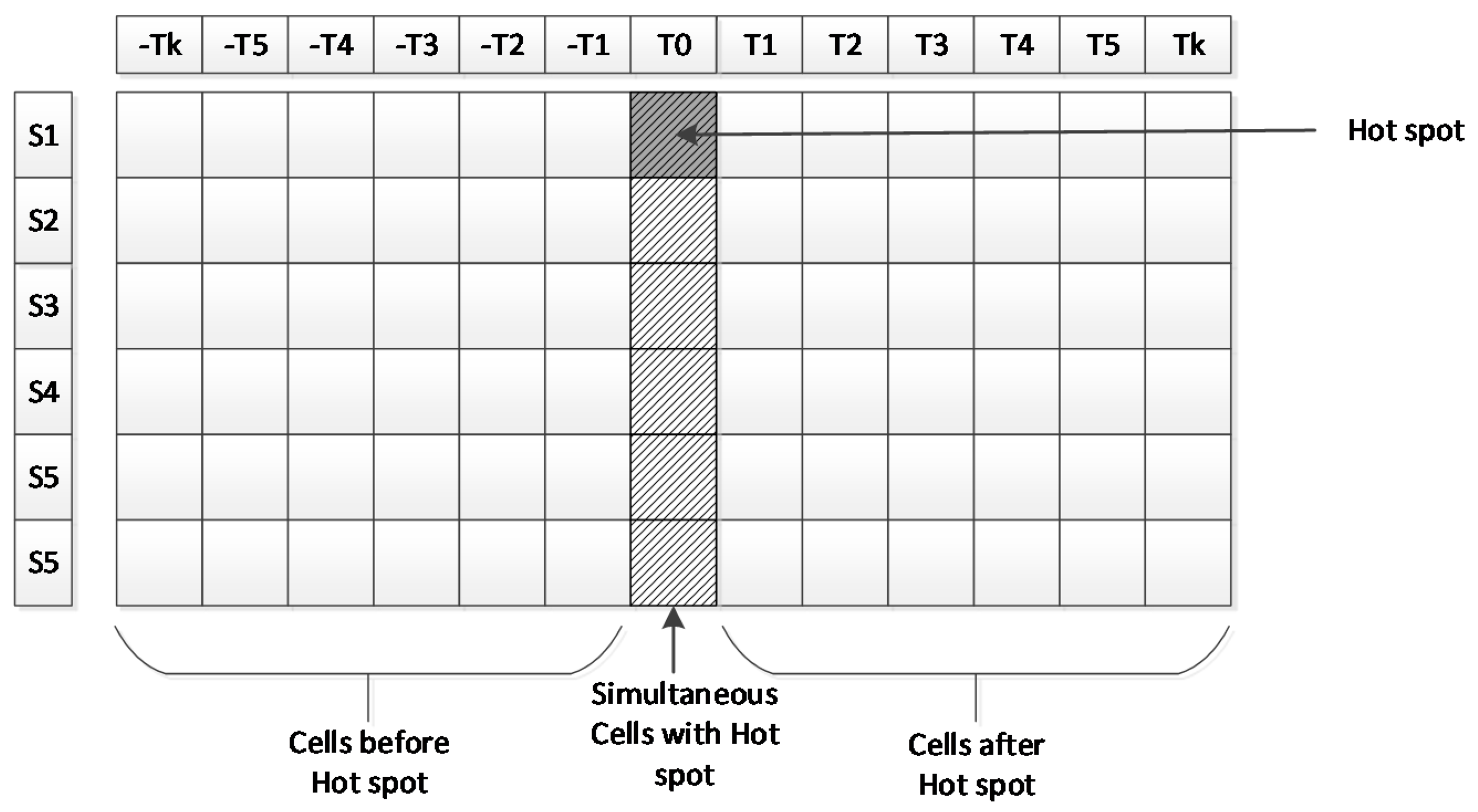
Based on the Knox test, the temporal expanded near repeat matrix (TENRM) was proposed to examine the risk undulation around a hotspot [8]. The difference between the TENRM and the near repeat matrix is that the hotspot will be situated at the initial position of the matrix rather than the event point. The temporal axis is expanded to record the risk undulation before hotspots (Figure 2). Similar to the RNR matrix, the horizontal and vertical axes in the temporal expanded near-repeat matrix indicate the space and time distance of risk around hotspots. Tk indicates the risk k temporal bands after hotspots, while Tk indicates the risk k temporal bands before hotspots. Sn is the nth spatial band away from hotspots.
In the construction of the TENRM, the hot spots will be detected by a quadrate search window. To fix the hotspot into the TENRM, the search window of hotspots should have the same space-time size as that of the TENRM. The definition and detect method of the hotspots in this research will follow existing research [41]. Each event point will be defined as the center of the space dimension and the starting point of the time dimension in the search window. The distribution of event numbers in the search window is hypothesized to follow a Poisson distribution. A null hypothesis test will be performed to examine the possibility of the event counts by a Poisson distribution. The probability of determining the specified count of events can be calculated with the equation:
where is the expected count of the event within the search window , A is the research area, and n is the number of all incidents. The cumulative probability of having at least number of events observed in is
A cluster of events will be recognized as a hotspot when the P value is smaller than the significance level . In this situation, the null hypothesis will be rejected. When two hotspots are spatially and temporally adjacent to each other, they will be merged. The following steps will follow the Knox test. The starting point of each event pair will be replaced by hotspots. The hotspot-event pairs will be counted, tabulated, and compared against the Monte Carlo matrix to generate the TENRM.
3.4. Modification of Hotspot-Based Knox Test
To examine the impact of a hotspot on the undulation of the risk of different crime types, the TENRM will be further modified. In contrast to the distance calculated within the same crime type in the TENRM, the modified Knox test will calculate the distance between hotspots and crimes by distinct type. Subsequently, a contingency table, in which each cell represents the count of distances between hotspots and crimes of a different type, will be computed. The Monte Carlo simulation will be employed to generate the expected distribution. Similar to the method proposed by Johnson et al., the further modified hotspot-based Knox test will only calculate the distance between hotspots and crimes by distinct crime type [10]. The expected distribution will be used to determine the expected value of each cell and the significance of the cell values in the near-repeat matrix.
3.5. Validity Threats
The study area is a typical large Chinese city. The urban development, economic status, and demographic characteristics make this city representative in Chinese cities. The crime pattern is reportedly similar to that of other large Chinese cities [8,15,20]. The interaction effect between different crime types, as of the research motivation in this study, can be inferred based on the existing theories and knowledge in existing research [17,18,19,20]. The current study is a further investigation based on the existing research. Getis-Ord Gi* statistic is a classic hotspot identification method. The Knox test is one of the most commonly used methods for detecting the spatial-temporal relationship between crimes. The utilization of the two methods for the identification of hotspots and interaction effects could double the reliability of the results.
As the current study incorporates raster grid cells, the modifiable areal unit problem (MAUP) is a potential risk factor to be discussed. The MAUP can alter research results by differing spatial resolutions and changing spatial boundaries. Due to the existence of MAUP, the RNR phenomenon has been examined in several spatial-temporal units [40,41,42,43]. The literature indicates that RNR exists on several spatial-temporal resolutions. According to the existing research, the 100 m × 7 days unit is mostly used and will be adopted in current research.
4. Study Area and Crime Data
4.1. Study Area
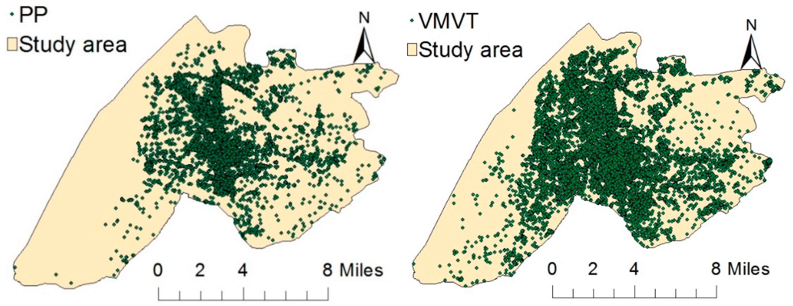
The study area (31°14′ E–32°37′ E, 118°22′ N–119°14′ N) is located in the economically developed Yangtze River Delta region and encompasses a total area of 263.43 km2 (Figure 2). As the capital of J province, N city is a core transportation hub. Efficient transportation enables transport to N city from other cities in the Yangtze River Delta region within one hour. N is composed of four districts. The central area has retained a large number of ancient buildings. The southwestern suburbs house an economic development zone with many new buildings. A city with both ancient and new buildings is very common in China’s big cities. N has a continental climate where the mean temperature is 15.6 °C and the annual precipitation varies between 534 mm and 1825.8 mm. Geographical advantages have enabled N city’s economy to rapidly develop like many other big cities in China. These economic and environmental characteristics make N highly representative in China. As a large city in the Yangtze River economic zone of China, N city offers an important contrast to evidence derived from previous studies conducted in other cities of China and elsewhere in the world.
4.2. Data Resources
The research data in this study were acquired from the Public Security Bureau (PSB) of N city. This data was generated from the 110 Emergency Response System (ERS). The crimes were addressed with a manual geocoding process. Finally, nearly 97.64% of all incidents were successfully geocoded.
The complete dataset includes a total of 10,012 PPs and 14,267 VMVTs recorded from January 1st, 2015, to December 30th, 2015. Each data record includes information about the victimization and its location (XY coordinates). All crimes are registered on the map based on the recorded coordinates, and the full dataset is used to quantitatively analyze the displacement of crimes in hot areas.
The PPs and VMVTs have different distribution patterns. Most PPs are concentrated in the central area of city N, while the VMVTs are scattered (Figure 3). Especially at the lower left and upper left areas, there are very few PPs but many VMVTs. The different distribution pattern makes the interaction analysis between the two crime types more meaningful.
5. Analysis
5.1. Distribution of Hotspots of PP and VMVT
To examine the interaction effect between the two crime types, the hotspots of the two crime types were separately detected. Consistent with the hotspot type used in TENRM, the grid hot spot will be adopted in the following analysis. The Getis-Ord Gi* statistic will be adopted to identify hotspots [44,45].
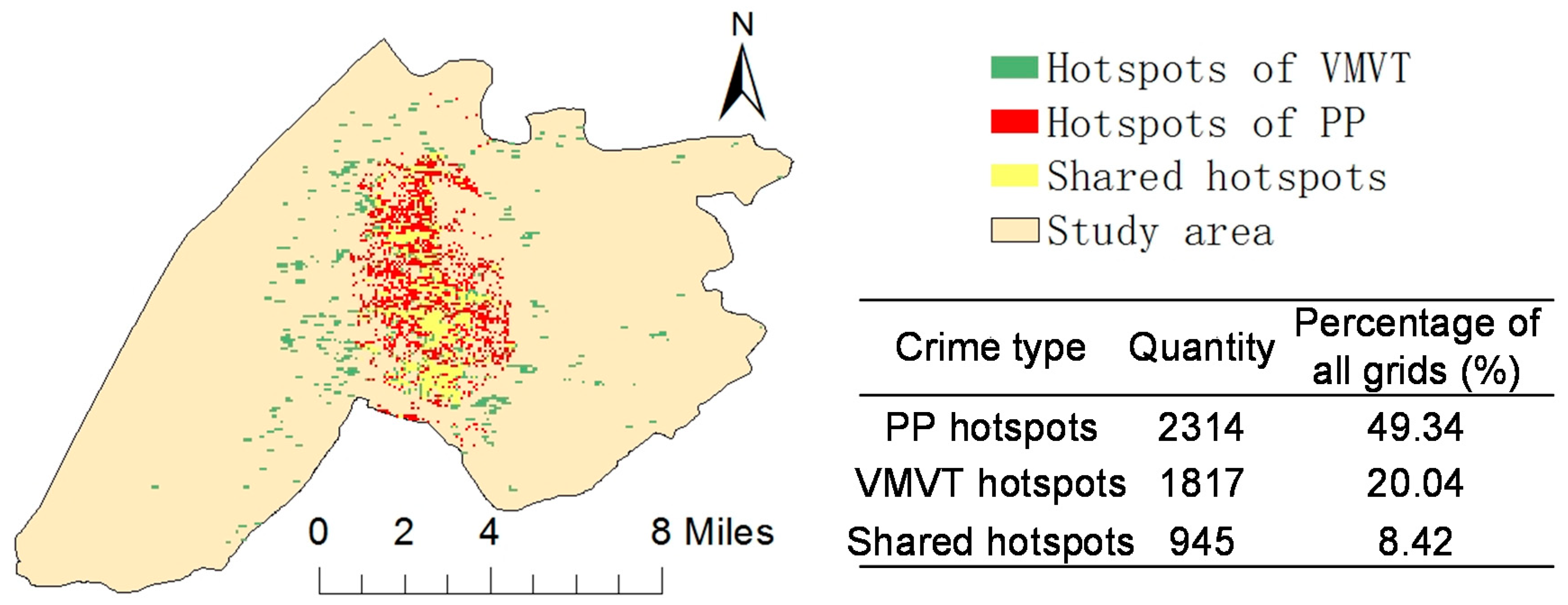
The distributions of the PP and VMVT are different (Figure 3). A total of 2314 grids are identified hotspots of PP. These hotspots are concentrated in the center part of the research area. Though fewer hotspots of VMVT are identified (1817), they spread over a larger area. However, the two crime types also share the same hotspots (945). The shared hotspots account for 8.42% of the research area. Therefore, a spatial interaction exists between the two crime types is shown in Figure 4.
5.2. Space-Time Interaction within Crime Type
The repeat and near-repeat phenomenon experimentally exist in PP crime (Table 1). The crime risk values are significantly higher than the expected values within 42 days in time and 1000 m in space. Within this space-time area, the risk values gradually decrease from the top left cell to the bottom right cell. These regular changed risk values indicate that the crime risk gradually decreases, with an increase in the distance and the elapsed time from a previous crime. Among the increased risk values, the largest value (3.09) is located at the top left corner of the matrix, which indicates that the risk level of another PP at the same location in 7 days is 3.09 times higher than the expected level. The elevated risk values concentrate within 14 days and 100 m from the previous PP crime. The RNR pattern of PP crime in this research is similar to current western and Asian research results.
The risk undulation after VMVT follows the same pattern of PP (Table 2). The RNR pattern also exists in the VMVT. In the matrix, the risk value gradually decreases from the top-left to the bottom-right. When one victimization is committed, the possibility of another victimization within 7 days at the same location is 2.22 times greater than the expected possibility. This high risk concentrates in 49 days within 100 m.
The two experiments indicate a significant RNR phenomenon among PP and VMVT in the large Chinese city. Therefore, crimes of the two types are spatially and temporally clustered. The conclusion is similar to the conclusions for the hotspots detected in previous research.
5.3. Space-Time Interaction across Crime Type
Table 3 and Table 4 portray the risk undulation after another type of crime. The experimental results indicate that the risk of another PP victimization is significantly high after every VMVT. The risk value of PP, which is located at the same location of the previous VMVT within one week, indicates a risk that is 2.47 times higher than normal risk values. The increased crime risk will continue for 7 weeks within a range of 100 m. The spatial extent with increased risk is limited. This result indicates that the risk of PP victimization will be significantly high even after 7 weeks at the locations or within 100 m of the previous VMVT.
In contrast to Table 3, Table 4 portrays the risk of VMVT after each PP. The highest risk of PP occurs immediately after one VMVT reaches 2.52 times (the top-left cell). Similar to Table 3, the increased crime risk continues for 7 weeks within 100 m.
The data in Table 3 and Table 4 conclude that PP victimizations and VMVT victimizations have a spatial-temporal interaction in this study area. The increased risk after each of the other crimes continue for 7 weeks within 100 m. When one crime occurs, the risk of another type of crime will increase and continue for 7 weeks within 100 m. Note that the small area of high risk after every other crime deserves more attention, as the narrowed spatial extent is valuable for crime prediction. Compared with the risk value (2.22) of VMVT in the RNR test (Table 2), the increased risk of VMVT after PP (2.52) seems to be higher. PP victimization may have a better ability of prediction for the next VMVT.
5.4. Impact of Hotspots across Crime Types
The period of 7 weeks remains at high risk within 100 m after the VMVT hotspot. Compared with the corresponding values in Table 3, the values within ‘0–42 days’ at ‘same location’ and ‘1–100 m’ are generally larger. For example, the risk value ranges from ‘8–14 days; the same location’ cell is 2.41;’ and the corresponding value in Table 3 is 2.32. The risk value ranges from ‘0–7 days; the 1–100 m’ cell is 1.38;’ and the corresponding value in Table 3 is 1.15. The differences indicate that when a VMVT victimization hotspot occurs, the possibility of PP in the following several weeks within 100 m will increase more than the risk after a VMVT victimization. Additional differences exist between Table 3 and Table 5. After the VMVT hotspots, a distanced area (>300 m) will also be subjected to high risk. This risk will continue for 7 weeks. This result completely differs from that in Table 3. In the left half of Table 5, the majority part of the left half matrix is not significant; the ‘same location’ and ‘1–100’ bands are not expected. This distribution of PP risk indicates that the PP risk concentrates with 100 m before VMVT hotspots. After the occurrence of VMVT hotspots, the PP risk will increase in the area within 100 m and a distanced area (>300 m) from VMVT hotspots. The increased risk will last for several weeks. Therefore, the VMVT hotspot can substantially change the risk of PP.
The VMVT risk after a PP hotspot does not considerably change at the same location compared with the VMVT risk after single PP victimization. For example, from 8–14 days, the cell of the same location in Table 6 is 2.29, while the corresponding band in Table 4 has the same value. The values in the band ‘1–100 m’ are larger than the corresponding values in Table 4. When a PP hotspot occurs, the possibility of another VMVT victimization in the area of ‘1–100 m’ will increase for several weeks. In contrast to Table 5, the large risk values comprise the majority cells of the left half part of Table 6. Before the occurrence of PP hotspots, many locations (same location, >300 m) are subject to a high risk of VMVT victimization. When the PP hotspots appear, the risk of another VMVT will concentrate within 100 m. Therefore, a PP hotspot can change the distribution of VMVT risk.
The experiment on the impact of crime hotspots on crime risk of another crime type indicates further interaction between the two crime types. After one hotspot, the risk of another crime type will probably increase more than the risk after a single crime of another type. The distribution of crime risk will also change after the hotspots of another crime type.
6. Discussion
In this research, the relationship between the two crime types was further investigated. The three questions about this relationship were answered by several experiments.
First, the phenomenon of RNR in PP and bicycle and motor bicycle theft were experimentally suggested—probably the first attempt—to exist in a large Chinese city. The existence of RNR has been experimentally examined with many types of crimes in current research [4,10,46,47,48,49]. Few studies have investigated RNR with the two types of crimes. The research results indicate that both types of crimes tend to be spatially clustered. When one crime victimization occurs, the same victimization will probably occur at the same location or locations in the vicinity in the following period. The boost and flag hypothesis may account for this cluster of crimes [3,40]. Based on the boost hypothesis, experienced offenders are more inclined to commit serial crimes within the adjacent spatial-temporal extent. The flag hypothesis argues that some particular attributes of vulnerable objects will be flagged to attract potential offenders. Both hypotheses can be employed to interpret the existence of an RNR pattern in the two crime types in a public area.
For the second question, interaction occurs between the two types of crimes. The spatial extent with increased risk after another type of crime occurs is limited within 100 m. Combined with the results from Figure 3, the findings concluded that the two types of crimes are spatially clustered. Note that the narrow spatial extent deserves more attention due to its potential ability to benefit crime prediction and policing patrol. This result indicates a strong interaction between the two crime types. The possibility of another VMVT victimization after PP may be higher than that after a previous VMVT. Subsequently, PP victimization may have a better ability to predict VMVT victimizations. The results can be interpreted as a displacement of modus operandi between two types. The interaction between the two crime types can be reasonably determined. Both PP and vehicle/motor vehicle theft are usually committed in crowded public places. A dense crowd provides a large number of objects for potential pocket-pickers and other thieves. Most of these public areas are crowded with people and bicycle/motor bicycles and provide numerous targets for both potential offenders. Consider bus stops as an example. A large number of people take buses every day. A high percentage of these people will ride/drive the distance from their homes to the bus stops. Therefore, these bus stops in a large city become gathering places for a large number of passengers and their different means of transport [26]. The spatially overlapped objects cause a strong interaction among potential offenders and a large proportion of overlapped hotspots of the crime types. The spatially limited interaction may increase the interaction and transformation between the two crimes types. Since the objects of two crime types are similar, the information or experience acquired from one crime type can easily be learned by the potential offenders of another crime type. The previously mentioned reasons produce a strong interaction between the two types of crimes. This result is different from that of the existing research [10]. This gap is attributed to the different crime types in the study. Burglary and theft from motor bicycle are two distinct crime types in terms of modus operandi and their location. PP and VMVT are similar for crime locations and acquired experience. Thus, further research is “warranted to determine the existence of the interaction” among other crime types [10].
Following to the third question, the risk undulation of one crime type after another crime type was also investigated. The impact of the two crime types on each other are similar; when a hotspot of one crime type appears, the possibility of another crime will increase. This finding supports the interaction between the two crime types. In addition, the increase in risk after hotspots of another crime type can be interpreted as modus operandi displacement. The offenders can change their targets after experiencing the high crime risk, even of another type. Some differences are observed in the impact of hotspots of one crime type on the risk of other crime types. After the hotspots of VMVT, the risk area of PP spreads to distanced locations (>300 m) from the limited area (<100 m). Conversely, the risk area of VMVT after PP hotspots converge from a large area (<100 m and >300 m) to a limited area (<100 m). The reason for this difference should be caused by the different distributions of targets of the two types of potential offenders. The bicycle and motor bicycles are usually parked at specified areas in the large Chinese city. The crimes cannot spatially displace a large amount. Conversely, the potential offenders of PP usually search for targets in pedestrians or crowd, which can distribute in a wider range of area than a parking area. Risk-avoiding activities occur within the area between 100 m and 300 m. Therefore, the risk can be transferred across crime types.
7. Conclusions
According to the crime data in N city, the PP and VMVT are spatially and temporally correlated. Based on the analysis, this correlation is caused by the shared similarities between the two crime types. The ‘boost’ hypothesis can account for this correlation. After one crime is committed, the other type of crime may be boosted soon due to the experience of the environment learned from a previous crime. Based on routine activity theory, the distribution of crowds and bicycle/motor bicycle parking areas are determined by people’s routine activities [19]. The potential offenders wander around the targeted areas until sufficient conditions (co-presented unprotected target and motivated offenders) are fulfilled [20]. The increased risk will last more than 7 weeks within 100 m. The limited spatial extent is separately determined by the spatial distribution of the targets in the two crime types. The narrowed spatial extent of crime risk after another type of crime deserves more attention due to its potential ability to improving crime prediction. After a hotspot, the crime risk of another type will increase and spatially and temporally displace to distanced areas. This risk avoiding activity is similar to that in the results in current research [8]. This distribution pattern of crime risk will benefit crime prediction and policing patrol.
This research has some drawbacks. Only two types of crime were employed in this study. Therefore, further research is warranted to examine whether the analyzed patterns exist among other crime types. Compared with the extensive research on crime patterns, a crime prediction model based on the explored crime patterns is needed.
Author Contributions
Conceptualization, Methodology—Zengli Wang; Validation—Hong Zhang
Funding
This research was funded by the National Natural Science Foundation of China (No. 41501488, 41471372, 41601422).
Acknowledgments
The authors would like to acknowledge the editor and anonymous reviewers for their insightful and constructive comments. The authors would also like to acknowledge the Public Security Bureau of N city for providing crime data.
Conflicts of Interest
The authors declare no conflict of interest.
References
- Anderson, D.; Chenery, S.; Pease, K. Biting Back: Tackling Repeat Burglary and Car Crime; Home Office Police Research Group: London, UK, 1995. Available online: https://www.ncjrs.gov/App/Publications/abstract.aspx?ID=154489 (accessed on 4 May 2019).
- Farrell, G.; Pease, K. Once Bitten, Twice Bitten: Repeat Victimisation and Its Implications for Crime Prevention. Crown Copyright. 1993. Available online: https://dspace.lboro.ac.uk/dspace-jspui/bitstream/2134/2149/1/Once_Bitten.pdf (accessed on 4 May 2019).
- Bowers, K.J.; Johnson, S.D. Who Commits Near Repeats? A Test of the Boost Explanation. West. Criminol. Rev. 2004, 5, 12–24. [Google Scholar]
- Ratcliffe, J.H.; Rengert, G.F. Near-repeat patterns in Philadelphia shootings. Secur. J. 2008, 21, 58–76. [Google Scholar] [CrossRef]
- Haberman, C.P.; Ratcliffe, J.H. The predictive policing challenges of near repeat armed street robberies. Policing J. Policy Pract. 2012, 6, 151–166. [Google Scholar] [CrossRef]
- Jochelson, R. Crime and Place: An Analysis of Assaults and Robberies in Inner Sydney. NSW Bureau of Crime Statistics and Research, Attorney General’s Department. 1997. Available online: https://www.bocsar.nsw.gov.au/Documents/r43.pdf (accessed on 4 May 2019).
- Townsley, M.; Homel, R.; Chaseling, J. Infectious burglaries. A test of the near repeat hypothesis. Br. J. Criminol. 2003, 43, 615–633. [Google Scholar] [CrossRef]
- Wang, Z.; Liu, X. Analysis of burglary hot spots and near-repeat victimization in a large Chinese city. ISPRS Int. J. Geo-Inf. 2017, 6, 148. [Google Scholar] [CrossRef]
- Nakaya, T.; Yano, K. Visualising crime clusters in a space-time cube: An exploratory data-analysis approach using space-time kernel density estimation and scan statistics. Trans. GIS 2010, 14, 223–239. [Google Scholar] [CrossRef]
- Johnson, S.D.; Summers, L.; Pease, K. Offender as forager? A direct test of the boost account of victimization. J. Quant. Criminol. 2009, 25, 181–200. [Google Scholar] [CrossRef]
- Clarke, R.V.; Harris, P.M. Auto theft and its prevention. Crime Justice 1992, 16, 1–54. [Google Scholar] [CrossRef]
- Clarke, R.V.; Harris, P.M. A rational choice perspective on the targets of automobile theft. Crim. Behav. Ment. Health 1992, 2, 25–42. [Google Scholar] [CrossRef]
- Pease, K. Repeat Victimisation: Taking Stock; Home Office Police Research Group: London, UK, 1998. Available online: https://www.ncjrs.gov/App/abstractdb/AbstractDBDetails.aspx?id=177325 (accessed on 4 May 2019).
- Johnson, S.D. Repeat burglary victimisation: A tale of two theories. J. Exp. Criminol. 2008, 4, 215–240. [Google Scholar] [CrossRef]
- Wu, L.; Xu, X.; Ye, X. Repeat and near-repeat burglaries and offender involvement in a large Chinese city. Cartogr. Geogr. Inf. Sci. 2015, 42, 178–189. [Google Scholar] [CrossRef]
- Bernasco, W. Them again? Same-offender involvement in repeat and near repeat burglaries. Eur. J. Criminol. 2008, 5, 411–431. [Google Scholar] [CrossRef]
- Brantingham, P.L.; Brantingham, P.J. Nodes, paths and edges: Considerations on the complexity of crime and the physical environment. J. Environ. Psychol. 1993, 13, 3–28. [Google Scholar] [CrossRef]
- Kinney, J.B.; Brantingham, P.L.; Wuschke, K. Crime attractors, generators and detractors: Land use and urban crime opportunities. Build Environ. 2008, 34, 62–74. [Google Scholar] [CrossRef]
- Cohen, L.E.; Felson, M. Social change and crime rate trends: A routine activity approach. Am. Sociol. Rev. 1979, 44, 588–608. [Google Scholar] [CrossRef]
- Bernasco, W. Foraging strategies of homo criminals: Lessons from behavioral ecology. Crime Patterns Anal. 2009, 2, 5–16. [Google Scholar]
- Etherington, N. Natal’s black rape scare of the 1870s. J. Southern Afr. Stud. 1988, 15, 36–53. [Google Scholar] [CrossRef]
- Huang, Y.; Chen, Y. A theft was changed to robbery after the car was stolen. Leg. Syst. Econol. 2008, 9, 46. [Google Scholar]
- Eck, J. The threat of crime displacement. Crim. Justice Abstr. 1993, 25, 527–546. [Google Scholar]
- Henry, L.M.; Bryan, B.A. Visualising the Spatio-Temporal Patterns of Motor Vehicle Theft in Adelaide, South Australia. Available online: https://digital.library.adelaide.edu.au/dspace/bitstream/2440/36277/1/henry.pdf (accessed on 4 May 2019).
- Lu, Y. Getting away with the stolen vehicle: An investigation of journey-after-crime. Prof. Geogr. 2003, 55, 422–433. [Google Scholar] [CrossRef]
- Johnson, S.D.; Summers, L.; Pease, K. Vehicle Crime: Communicating Spatial and Temporal Patterns. UCL JILL DANDO Institute of Crime Science. 2006. Available online: http://discovery.ucl.ac.uk/1430754/1/2006_JDI_Vehicle_Crime.pdf (accessed on 4 May 2019).
- Lockwood, B. The presence and nature of a near-repeat pattern of motor vehicle theft. Secur. J. 2012, 25, 38–56. [Google Scholar] [CrossRef]
- Plouffe, N.; Sampson, R. Auto theft and theft from autos in parking lots in Chula Vista, CA: Crime analysis for local and regional action. Underst. Prev. Car Theft Crime Prev. Stud. 2004, 17, 147–171. [Google Scholar]
- Rengert, G.F.; Piquero, A.R.; Jones, P.R. Distance decay reexamined. Criminology 1999, 37, 427–446. [Google Scholar] [CrossRef]
- Sallybanks, J.; Brown, R. Vehicle Crime Reduction: Turning the Corner; Home Office, Policing and Reducing Crime Unit, Research, Development and Statistics Directorate: London, UK, 1999; Available online: http://citeseerx.ist.psu.edu/viewdoc/download?doi=10.1.1.514.3654&rep=rep1&type=pdf (accessed on 4 May 2019).
- Levine, N.; Wachs, M.; Shirazi, E. Crime at bus stops: A study of environmental factors. J. Archit. Plan. Res. 1986, 3, 339–361. [Google Scholar]
- De Albuquerque, K.; McElroy, J. Tourism and crime in the Caribbean. Ann. Tour. Res. 1999, 26, 968–984. [Google Scholar] [CrossRef] [Green Version]
- Bunting, R.J.; Chang, O.Y.; Cowen, C. Spatial patterns of larceny and aggravated assault in Miami–Dade County, 2007–2015. Prof. Geogr. 2018, 70, 34–46. [Google Scholar] [CrossRef]
- Shannon, L.W. The spatial distribution of criminal offenses by states. J. Crim. Law Criminol. Police Sci. 1954, 45, 264–273. [Google Scholar] [CrossRef]
- Song, G.; Liu, L.; Bernasco, W. Testing indicators of risk populations for theft from the person across space and time: The significance of mobility and outdoor activity. Ann. Am. Assoc. Geograph. 2018, 108, 1370–1388. [Google Scholar] [CrossRef]
- Liu, L.; Feng, J.; Ren, F. Examining the relationship between neighborhood environment and residential locations of juvenile and adult migrant burglars in China. Cities 2018, 82, 10–18. [Google Scholar] [CrossRef]
- Liu, L.; Jiang, C.; Zhou, S. Impact of public bus system on spatial burglary patterns in a Chinese urban context. Appl. Geogr. 2017, 89, 142–149. [Google Scholar] [CrossRef]
- Knox, G. The detection of space-time interactions. Appl. Stat. 1964, 13, 25–29. [Google Scholar] [CrossRef]
- Johnson, S.D.; Bowers, K.J. Burglary prediction: Theory, flow and friction. In Imagination for Crime Prevention: Essays in Honour of Ken Pease, Vol. 21 of Crime Prevention Studies; Farrell, G., Bowers, K.J., Johnson, S.D., Townsley, M., Eds.; Criminal Justice Press: Monsey, NY, USA, 2007; pp. 203–223. Available online: http://discovery.ucl.ac.uk/76545/ (accessed on 4 May 2019).
- Chainey, S.P.; Braulio, F.A.da.S. Examining the extent of repeat and near repeat victimisation of domestic burglaries in Belo Horizonte, Brazil. Crime Sci. 2016, 5, 1. [Google Scholar] [CrossRef]
- Shiode, S.; Shiode, N. Network-based space-time search-window technique for hotspot detection of street-level crime incidents. Int. J. Geogr. Inf. Sci. 2013, 27, 866–882. [Google Scholar] [CrossRef]
- Farrell, G.; Bouloukos, A.C. International overview: A cross-national comparison of rates of repeat victimization. Crime Prev. Stud. 2001, 12, 5–26. [Google Scholar]
- Chainey, S.P. Examining the Extent to Which Hotspot Analysis Can Support Spatial Predictions of Crime; UCL (University College London): London, UK, 2014; Available online: http://discovery.ucl.ac.uk/1458643/1/SChainey%20PhD%20Final%20Version.pdf (accessed on 4 May 2019).
- Getis, A.; Ord, J.K. The Analysis of Spatial Association by Use of Distance Statistics. Geogr. Anal. 1992, 24, 189–206. [Google Scholar] [CrossRef]
- Ord, J.K.; Getis, A. Local spatial autocorrelation statistics: Distributional issues and an application. Geogr. Anal. 1995, 27, 286–306. [Google Scholar] [CrossRef]
- Short, M.B.; D’orsogna, M.R.; Brantingham, P.J.; Tita, G.E. Measuring and modeling repeat and near-repeat burglary effects. J. Quant. Criminol. 2009, 25, 325–339. [Google Scholar] [CrossRef]
- Johnson, S.D.; Bernasco, W.; Bowers, K.J. Space–time patterns of risk: A cross national assessment of residential burglary victimization. J. Quant. Criminol. 2007, 23, 201–219. [Google Scholar] [CrossRef]
- Melo, S.N.; Andresen, M.A.; Matias, L.F. Repeat and near-repeat victimization in Campinas, Brazil: New explanations from the Global South. Secur. J. 2018, 31, 364–380. [Google Scholar] [CrossRef]
- Glasner, P.; Johnson, S.D.; Leitner, M. A comparative analysis to forecast apartment burglaries in Vienna, Austria, based on repeat and near repeat victimization. Crime Sci. 2018, 7, 9. [Google Scholar] [CrossRef] [PubMed]
Figure 1.
Demonstration of current research.

Figure 2.
Diagram of temporal expanded near-repeat algorithm.

Figure 3.
Overview of the study area and two crime types (pocket-picking (PP) and (vehicle, motor vehicle theft) VMVT).
Figure 3.
Overview of the study area and two crime types (pocket-picking (PP) and (vehicle, motor vehicle theft) VMVT).

Figure 4.
Hotspots of two crime types.


Table 1.
Repeat and near-repeat (RNR) matrix of PP.
| Distance (meters) | 0–7 days | 8–14 days | 15–21 days | 22–28 days | 29–35 days | 36–42 days | >43 days |
|---|---|---|---|---|---|---|---|
| Same location | 3.09 ** | 2.66 ** | 2.45 ** | 2.27 ** | 2.13 ** | 1.82 ** | 1.55 ** |
| 1–100 | 1.59 ** | 1.43 ** | 1.36 ** | 1.30 ** | 1.22 ** | 1.18 ** | 1.08 * |
| 101–200 | 1.34 ** | 1.26 ** | 1.22 ** | 1.14 ** | 1.12 ** | 1.10 ** | 1.01 |
| 201–300 | 1.32 ** | 1.24 ** | 1.20 ** | 1.13 ** | 1.12 ** | 1.06 ** | 1.02 |
| 301–400 | 1.30 ** | 1.23 ** | 1.18 ** | 1.17 ** | 1.12 ** | 1.06 ** | 1.01 |
| 401–500 | 1.23 ** | 1.19 ** | 1.13 ** | 1.10 * | 1.07 ** | 1.06 ** | 1.01 |
| 501–600 | 1.25 ** | 1.20 ** | 1.16 ** | 1.12 ** | 1.10 ** | 1.05 ** | 0.99 |
| 601–700 | 1.27 ** | 1.20 ** | 1.16 ** | 1.11 * | 1.07 * | 1.05 ** | 1.01 |
| 701–800 | 1.23 ** | 1.14 ** | 1.11 ** | 1.08 * | 1.04 * | 1.03 * | 0.98 |
| 801–900 | 1.25 ** | 1.19 ** | 1.15 ** | 1.10 * | 1.08 ** | 1.03 * | 0.98 |
| 901–1000 | 1.24 ** | 1.17 ** | 1.14 ** | 1.11 ** | 1.07 * | 1.02 | 0.98 |
| >1000 | 1.21 ** | 1.17 * | 1.12 * | 1.10 * | 1.07 * | 1.03 * | 0.98 |
Note: * p < 0.01. ** p < 0.001.
Table 2.
RNR matrix of VMVT.
| Distance (meters) | 0–7 days | 8–14 days | 15–21 days | 22–28 days | 29–35 days | 36–42 days | >43 days |
|---|---|---|---|---|---|---|---|
| Same location | 2.22 ** | 2.08 ** | 1.95 ** | 1.86 ** | 1.71 ** | 1.68 ** | 1.54 ** |
| 1–100 | 1.32 ** | 1.26 ** | 1.21 ** | 1.19 ** | 1.17 ** | 1.15 ** | 1.15 * |
| 101–200 | 1.08 ** | 1.07 ** | 1.03 * | 1.01 | 1.03 * | 1.03 | 1.02 |
| 201–300 | 1.05 * | 1.04 * | 1.04 * | 1.04 * | 1.05 * | 1.05 * | 1.04 * |
| 301–400 | 1.05 * | 1.05 * | 1.06 * | 1.03 * | 1.05 * | 1.05 * | 1.04 * |
| 401–500 | 1.04 * | 1.04 * | 1.04 * | 1.02 * | 1.03 * | 1.03 * | 1.04 * |
| 501–600 | 1.07 ** | 1.05 * | 1.04 * | 1.05 * | 1.03 * | 1.03 * | 1.05 * |
| 601–700 | 1.05 * | 1.05 * | 1.06 * | 1.04 * | 1.03 * | 1.04 * | 1.05 * |
| 701–800 | 1.05 * | 1.04 * | 1.03 * | 1.03 * | 1.03 * | 1.04 * | 1.03 * |
| 801–900 | 1.05 * | 1.03 * | 1.03 * | 1.04 * | 1.02 * | 1.03 * | 1.05 * |
| 901–1000 | 1.05 * | 1.03 * | 1.03 * | 1.02 * | 1.03 * | 1.04 * | 1.03 * |
| >1000 | 1.04 * | 1.03 * | 1.03 * | 1.03 * | 1.03 * | 1.03 * | 1.04 * |
Note: * p < 0.01. ** p < 0.001.
Table 3.
Risk of PP after VMVT.
| Distance (meters) | 0–7 days | 8–14 days | 15–21 days | 22–28 days | 29–35 days | 36–42 days | >43 days |
|---|---|---|---|---|---|---|---|
| Same location | 2.47 ** | 2.32 ** | 2.27 ** | 2.39 ** | 2.17 ** | 2.12 ** | 2.21 ** |
| 1–100 | 1.15 ** | 1.13 ** | 1.16 ** | 1.12 ** | 1.14 ** | 1.12 ** | 1.15 ** |
| 101–200 | 0.98 | 0.95 | 0.94 | 0.95 | 0.96 | 0.97 | 0.96 |
| 201–300 | 0.98 | 0.97 | 0.97 | 0.97 | 0.96 | 0.98 | 0.97 |
| 301–400 | 0.99 | 0.99 | 0.99 | 1.03 | 1.00 | 1.00 | 1.02 |
| 401–500 | 0.97 | 0.97 | 0.97 | 0.99 | 0.96 | 0.97 | 0.98 |
| 501–600 | 0.99 | 1.00 | 0.99 | 1.00 | 0.97 | 1.00 | 0.98 |
| 601–700 | 0.99 | 0.99 | 1.01 | 1.02 * | 1.00 | 1.00 | 1.02 |
| 701–800 | 0.98 | 0.98 | 0.97 | 0.99 | 0.98 | 0.99 | 1.00 |
| 801–900 | 0.99 | 0.98 | 1.00 | 1.03 | 1.01 | 1.00 | 1.01 |
| 901–1000 | 0.99 | 0.99 | 0.98 | 1.01 | 0.99 | 1.00 | 1.00 |
| > 1000 | 0.98 | 0.97 | 0.98 | 0.99 | 0.98 | 0.98 | 0.98 |
Note: * p < 0.01. ** p < 0.001.
Table 4.
Risk of VMVT after PP.
| Distance (meters) | 0–7 days | 8–14 days | 15–21 days | 22–28 days | 29–35 Days | 36–42 days | >43 days |
|---|---|---|---|---|---|---|---|
| Same location | 2.52 ** | 2.29 ** | 2.1 ** | 1.88 ** | 1.92 ** | 1.71 ** | 1.53 ** |
| 1–100 | 1.16 ** | 1.11 ** | 1.12 ** | 1.12 ** | 1.09 ** | 1.08 ** | 1.08 ** |
| 101–200 | 1.00 * | 0.97 | 0.93 | 0.92 | 0.96 | 0.93 | 0.96 |
| 201–300 | 0.96 | 0.98 | 0.96 | 0.94 | 0.95 | 0.96 | 0.98 |
| 301–400 | 1.00 | 0.98 | 0.98 | 0.97 | 0.96 | 0.98 | 0.99 |
| 401–500 | 0.96 | 0.97 | 0.97 | 0.95 | 0.95 | 0.96 | 0.98 |
| 501–600 | 0.99 | 0.98 | 0.98 | 0.97 | 0.99 | 0.98 | 0.98 |
| 601–700 | 1.00 | 1.00 | 0.99 | 0.98 | 0.99 | 0.97 | 1.00 |
| 701–800 | 0.98 | 0.98 | 0.96 | 0.96 | 0.96 | 0.98 | 0.98 |
| 801–900 | 1.00 | 1.00 | 0.99 | 0.99 | 0.98 | 0.98 | 0.99 |
| 901–1000 | 0.99 | 0.99 | 0.97 | 0.96 | 0.95 | 0.98 | 1.00 |
| >1000 | 0.98 | 0.97 | 0.97 | 0.96 | 0.96 | 0.97 | 0.98 |
Note: * p < 0.01. ** p < 0.001.
Table 5.
Risk of PP after VMVT hotspot.
| Distance (meters) | Past (day) | Same Time | Future (day) | ||||||||||||
|---|---|---|---|---|---|---|---|---|---|---|---|---|---|---|---|
| >42 | 36–42 | 29–35 | 22–28 | 15–21 | 8–14 | 0–7 | 0–7 | 8–14 | 15–21 | 22–28 | 20–35 | 36–42 | >42 | ||
| Same location | 0.33 | 0.96 | 1.21 ** | 1.46 ** | 1.63 ** | 1.99 ** | 2.26 ** | 2.66 ** | 2.50 ** | 2.41 ** | 2.52 ** | 2.63 ** | 2.31 ** | 2.31 ** | 2.54 ** |
| 1–100 | 0.74 | 0.92 | 1.10 | 1.14 * | 1.19 ** | 1.23 ** | 1.28 ** | 1.39 ** | 1.38 ** | 1.42 ** | 1.45 ** | 1.43 ** | 1.42 ** | 1.50 ** | 1.60 ** |
| 101–200 | 0.96 | 0.79 | 0.76 | 0.82 | 0.81 | 0.84 | 0.88 | 1.02 | 0.87 | 0.89 | 0.89 | 1.00 | 1.07 | 1.05 * | 1.06 |
| 201–300 | 0.94 | 0.80 | 0.73 | 0.77 | 0.87 | 0.88 | 0.92 | 0.95 | 1.01 | 0.98 | 0.98 | 1.00 | 1.04 | 1.07 | 1.08 * |
| 301–400 | 0.90 | 0.90 | 0.87 | 0.86 | 0.93 | 1.00 | 1.00 | 1.03 | 1.05 * | 1.05 * | 1.13 ** | 1.18 ** | 1.12 ** | 1.14 ** | 1.19 ** |
| 401–500 | 0.92 | 0.85 | 0.81 | 0.85 | 0.84 | 0.90 | 0.89 | 0.93 | 0.98 | 0.99 | 1.03 | 1.05 | 1.08 ** | 1.10 ** | 1.04 |
| 501–600 | 0.88 | 0.84 | 0.89 | 0.93 | 1.02 | 0.97 | 1.04 | 1.02 | 1.10 * | 1.14 ** | 1.17 ** | 1.13 ** | 1.16 ** | 1.18 ** | 1.11 ** |
| 601–700 | 0.84 | 0.94 | 0.90 | 0.96 | 0.99 | 1.07 | 1.07 ** | 1.11 ** | 1.08 ** | 1.17 ** | 1.20 ** | 1.17 ** | 1.12 ** | 1.22 ** | 1.19 ** |
| 701–800 | 0.90 | 0.81 | 0.86 | 0.87 | 0.89 | 0.86 | 0.94 | 0.98 | 0.96 | 1.05 | 1.03 | 1.07 ** | 1.09 ** | 1.14 ** | 1.15 ** |
| 801–900 | 0.87 | 0.87 | 0.92 | 0.99 | 1.01 | 1.04 | 1.08 ** | 1.16 ** | 1.16 ** | 1.16 ** | 1.20 ** | 1.27 ** | 1.21 ** | 1.20 ** | 1.22 ** |
| 901–1000 | 0.90 | 0.84 | 0.83 | 0.88 | 0.90 | 0.99 | 0.99 | 1.05 | 1.10 ** | 1.14 ** | 1.13 ** | 1.19 ** | 1.14 ** | 1.15 ** | 1.14 ** |
| >1000 | 0.89 | 0.84 | 0.87 | 0.90 | 0.93 | 0.96 | 0.99 | 1.04 ** | 1.07 ** | 1.10 ** | 1.13 ** | 1.16 ** | 1.16 ** | 1.16 ** | 1.16 ** |
Note: * p < 0.01. ** p < 0.001.
Table 6.
Risk of VMVT after a PP hotspot.
| Distance (meters) | Past (day) | Same Time | Future (day) | ||||||||||||
|---|---|---|---|---|---|---|---|---|---|---|---|---|---|---|---|
| >42 | 36–42 | 29–35 | 22–28 | 15–21 | 8–14 | 0–7 | 0–7 | 8–14 | 15–21 | 22–28 | 20–35 | 36–42 | >42 | ||
| Same location | 0.54 | 1.78 ** | 1.74 ** | 1.98 ** | 2.22 ** | 2.25 ** | 2.24 ** | 2.35 ** | 2.53 ** | 2.29 ** | 2.11 ** | 1.90 ** | 1.89 ** | 1.59 ** | 1.51 ** |
| 1–100 | 0.81 | 1.35 ** | 1.32 ** | 1.30 ** | 1.30 ** | 1.37 ** | 1.32 ** | 1.32 ** | 1.25 ** | 1.21 ** | 1.22 ** | 1.23 ** | 1.16 ** | 1.23 ** | 1.17 ** |
| 101–200 | 1.00 | 1.02 | 1.01 | 0.94 | 0.91 | 0.90 | 0.89 | 0.92 | 0.92 | 0.91 | 0.83 | 0.87 | 0.87 | 0.90 | 0.91 |
| 201–300 | 0.98 | 1.03 | 1.00 | 0.97 | 1.00 | 0.96 | 0.95 | 0.93 | 0.93 | 0.92 | 0.92 | 0.88 | 0.89 | 0.91 | 0.94 |
| 301–400 | 0.94 | 1.11 ** | 1.13 ** | 1.07 ** | 1.09 ** | 1.02 ** | 1.00 | 0.96 | 1.01 | 0.99 | 0.98 | 0.95 | 0.94 | 0.99 | 0.98 |
| 401–500 | 0.97 | 1.04 | 1.05 | 1.03 | 1.00 | 0.97 | 0.96 | 0.94 | 0.89 | 0.94 | 0.94 | 0.89 | 0.92 | 0.94 | 0.98 |
| 501–600 | 0.94 | 1.08 * | 1.11 ** | 1.03 | 1.07 ** | 1.05 ** | 1.03 | 1.02 | 1.02 | 0.98 | 1.00 | 1.00 | 1.00 | 1.02 | 0.99 |
| 601–700 | 0.91 | 1.16 ** | 1.08 | 1.08 * | 1.07 ** | 1.04 ** | 1.04 | 1.04 | 1.05 * | 1.02 | 1.03 | 1.03 * | 1.00 | 0.99 | 1.05 |
| 701–800 | 0.95 | 1.06 * | 1.06 | 0.99 | 1.00 | 0.99 | 0.96 | 0.94 | 0.98 | 0.95 | 0.92 | 0.94 | 0.96 | 0.98 | 0.97 |
| 801–900 | 0.92 | 1.12 ** | 1.08 | 1.06 * | 1.09 ** | 1.05 ** | 1.02 | 1.03 | 1.03 | 1.06 ** | 1.01 | 1.04 | 0.98 | 1.01 | 0.99 |
| 901–1000 | 0.94 | 1.10 ** | 1.13 ** | 1.07 ** | 1.06 * | 1.01 | 1.00 | 0.96 | 0.96 | 0.99 | 0.95 | 0.92 | 0.94 | 0.97 | 1.01 |
| >1000 | 0.96 | 1.08 ** | 1.06 ** | 1.05 ** | 1.04 ** | 1.02 ** | 0.99 | 0.97 | 0.96 | 0.95 | 0.94 | 0.93 | 0.94 | 0.94 | 0.96 |
Note: * p < 0.01. ** p < 0.001.
© 2019 by the authors. Licensee MDPI, Basel, Switzerland. This article is an open access article distributed under the terms and conditions of the Creative Commons Attribution (CC BY) license (http://creativecommons.org/licenses/by/4.0/).
Share and Cite
MDPI and ACS Style
Wang, Z.; Zhang, H. Could Crime Risk Be Propagated across Crime Types? ISPRS Int. J. Geo-Inf. 2019, 8, 203. https://0-doi-org.brum.beds.ac.uk/10.3390/ijgi8050203
AMA Style
Wang Z, Zhang H. Could Crime Risk Be Propagated across Crime Types? ISPRS International Journal of Geo-Information. 2019; 8(5):203. https://0-doi-org.brum.beds.ac.uk/10.3390/ijgi8050203
Chicago/Turabian StyleWang, Zengli, and Hong Zhang. 2019. "Could Crime Risk Be Propagated across Crime Types?" ISPRS International Journal of Geo-Information 8, no. 5: 203. https://0-doi-org.brum.beds.ac.uk/10.3390/ijgi8050203
Note that from the first issue of 2016, this journal uses article numbers instead of page numbers. See further details here.