Mobility Modes Awareness from Trajectories Based on Clustering and a Convolutional Neural Network

Abstract

Massive trajectory data generated by ubiquitous position acquisition technology are valuable for knowledge discovery. The study of trajectory mining that converts knowledge into decision support becomes appealing. Mobility modes awareness is one of the most important aspects of trajectory mining. It contributes to land use planning, intelligent transportation, anomaly events prevention, etc. To achieve better comprehension of mobility modes, we propose a method to integrate the issues of mobility modes discovery and mobility modes identification together. Firstly, route patterns of trajectories were mined based on unsupervised origin and destination (OD) points clustering. After the combination of route patterns and travel activity information, different mobility modes existing in history trajectories were discovered. Then a convolutional neural network (CNN)-based method was proposed to identify the mobility modes of newly emerging trajectories. The labeled history trajectory data were utilized to train the identification model. Moreover, in this approach, we introduced a mobility-based trajectory structure as the input of the identification model. This method was evaluated with a real-world maritime trajectory dataset. The experiment results indicated the excellence of this method. The mobility modes discovered by our method were clearly distinguishable from each other and the identification accuracy was higher compared with other techniques.

1. Introduction

The mobility behavior of users is the key factor for understanding the spatiotemporal characteristics of human activity, transportation conditions, and environment. Massive travels by users can be categorized into different modes, such as transportation modes (subway, bike, taxi, and bus, etc.) [1] and different frequent route patterns [2]. Distinguishing different mobility modes and understanding the character of them play a key role in location-based services such as destination and route prediction [3,4] and analysis of travel behavior [5], etc. Traditional ways of investigating mobility modes rely on household interviews and manual labelling, which are inefficient and costly.

With the rapid development of navigation and positioning technology, it has become feasible to acquire users’ trajectory data in real-time and in a consecutive manner. Valuable knowledge about the mobility behavior of users and the spatiotemporal characteristics of environment are contained in these data [6]. Ubiquitous trajectory data and great demand of decision support lead to the increasing advent of data-driven techniques for trajectory mining [7]. The recent literature on trajectory mining mainly focused on significant locations discovery, anomaly detection, location-based activity recognition, and mobility modes identification [1,8]. Trajectory mining also provides an opportunity to enhance the awareness of mobility modes. Our work considers the information of both travel activity types and route patterns to categorize different mobility modes. For example, a person travels from location A to location B by bus/taxi, or a vessel travels from port A to port B for tugging/carrying cargo.

The mobility modes introduced above are worth exploring since different modes contain abundant knowledge about not only the significant places [9] and route patterns [10], but also semantic information such as the travel activity types. Mobility modes awareness in this work involves two issues: mobility modes discovery and mobility modes identification. The former aims to mine different mobility modes existing in a large amount of history trajectories. This knowledge facilitates the intelligent management of both environment and travel behavior of users, such as land use classification [11] and anomalous trajectory detection [12]. The latter focuses on predicting the mobility mode of a newly emerging trajectory in real-time manner. Mobility modes identification is the basis of customized location-based service [13] and activity surveillance [14].

In order to mine valuable knowledge from history trajectory data and generate massive labeled data for the training of the identification model automatically, we propose an approach to integrate the issues of mobility modes discovery and identification together. This approach includes three successive components: trajectory preprocessing, clustering, and identification model training and evaluation. Firstly, we perform trajectory preprocessing to obtain clean data and prepare trajectories well for subsequent study. Then, we categorize history trajectories into different mobility modes in an unsupervised manner and tag them with labels. Further, in the phase of mobility modes identification, we construct and train an identification model offline by leveraging history trajectory data labeled before. The mobility mode of a newly emerging trajectory will be identified in real-time manner by this well-trained identification model. Although lots of previous literatures [15,16] have paid attention to the issues about mobility modes awareness, there still exists much space to explore. In this paper, we make an effort to efficiently discover distinguishable mobility modes and improve the performance of identification.

The crucial issue of mobility modes discovery is route pattern extraction. The most widely used way to mine route patterns is utilizing clustering-based approaches due to the similarity among trajectories in the same route pattern [17,18,19]. Ordering points to identify the clustering structure (OPTICS) algorithm is insensitive to parameters and more robust compared to other clustering algorithms [20]. In this work, we propose to extract route patterns by means of origin and destination (OD) points clustering based on OPTICS. One of the most prominent advantages of this method is the adaptive ability against density imbalance condition. Moreover, it can efficiently deal with the complicated trajectory behavior.

Accomplishing the identification task involves two key points. The first one is preparing trajectories for representative feature extraction. These features are supposed to be capable of adequately interpreting different modes. The second is constructing and training an identification model for feature learning and result prediction. This model is expected to identify different modes accurately on the basis of extracted representative features. In this work, we propose a deep learning approach to identify mobility modes based on a convolutional neural network (CNN). We introduce mobility-based structure for individual trajectories. Compared to an ordinary time-series trajectory structure, the superiority of a mobility-based structure is the simultaneous expression of comprehensive knowledge including the spatial and kinematic characteristics. A CNN, which is outstanding in the field of pattern identification, is also capable of extracting distinguishable features from mobility-based trajectory.

The principal contributions of our work are: (1) We propose a method aiming to integrate the issues of mobility modes discovery and identification together. It enhances the awareness of mobility behavior, which will be contributive in plenty of practical fields. (2) We put forward an efficient OD points clustering method based on OPTICS for mobility modes discovery. The discovered modes contain abundant knowledge about both spatial and semantic characteristics of moving objects. (3) We propose a deep learning approach for mobility modes identification, which automatically learns high-level features from trajectory data. This approach does not need any domain knowledge to develop sophisticated feature extractor and is easy to be transplanted to different situation. The introduction of mobility-based trajectory structure is also progressive. (4) Our work provides a typical way to convert trajectory big data into knowledge and decision support.

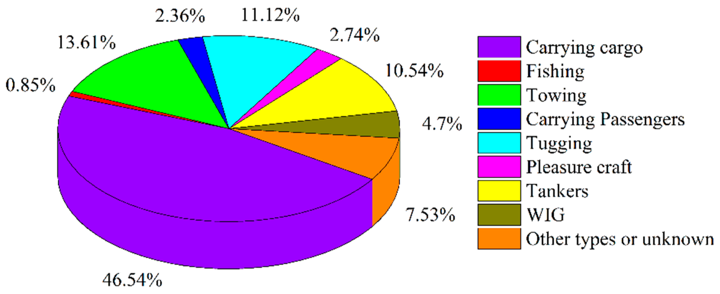
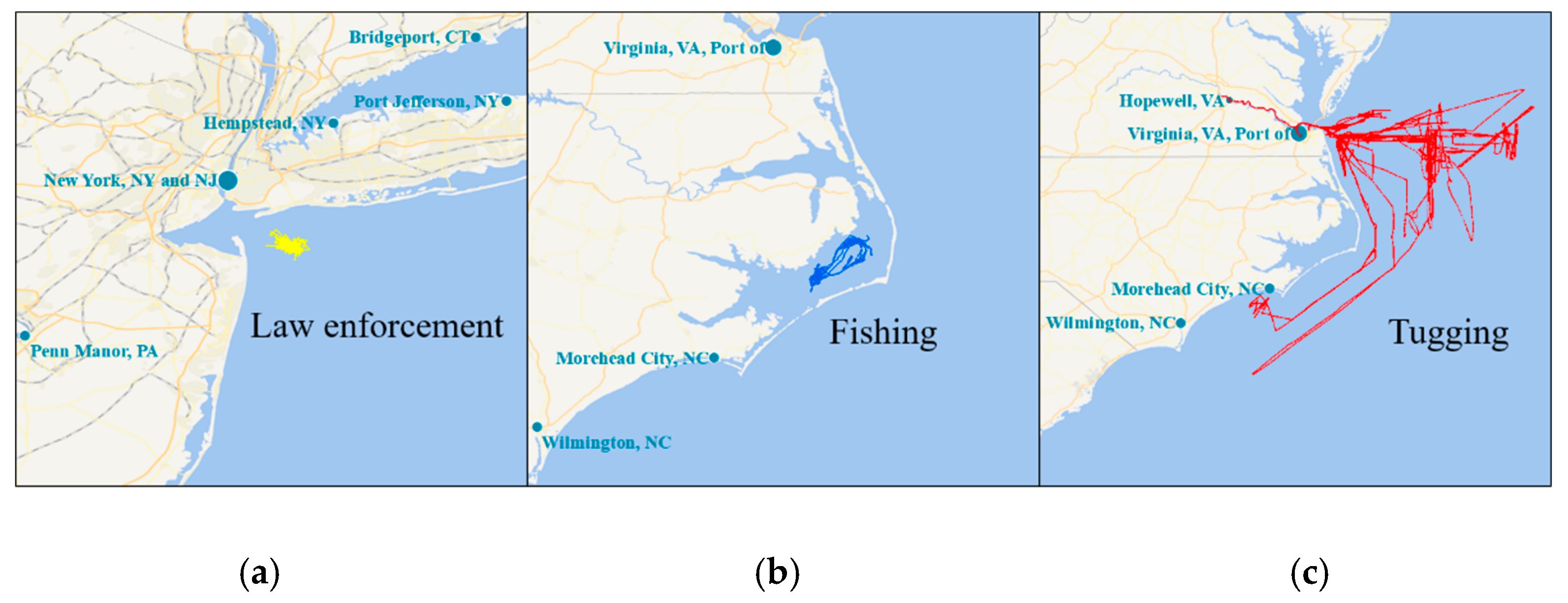
We employed real-world vessel trajectory data collected by an Automatic Identification System (AIS) [21] for the evaluation of the proposed method. The mobility modes defined above were composed of vessel route patterns and different maritime activity types in this specific case. The remainder of this paper is organized as follows. Section 2 reviews the related work on the investigation of mobility modes. In Section 3, the proposed methodology on mobility modes awareness is elaborated. Experiments and evaluation are presented in Section 4. This section also brings a visualization of extracted deep features. Ultimately, we discuss and conclude this work and also present future prospects in Section 5.

2. Related Work

Destination prediction from trajectories is a widely discussed issue which is usually derived from mobility modes awareness. In Reference [22], three steps were involved in the destination prediction issue: (1) obtain trajectory clusters and traffic pattern models, (2) assign the new trajectory to a particular cluster, and (3) predict the destination based on history information and current state. The first two steps can also be regarded as mobility modes awareness.

A specific mobility mode is formed by the behavior of a group of similar trajectories. Thus, clustering algorithms are the most widely used techniques for mobility modes discovery in previous studies. A comprehensive review on trajectory clustering categorized these algorithms into three groups [23]: unsupervised, supervised, and semi-supervised. The most intuitional way is taking the trajectory itself as clustering object [17,24,25]. A framework called hierarchical graph-based similarity measurement (HGSM) was proposed to mine the similarity between user trajectories geographically. The advantages of this framework lie in taking both the sequence property of people’s behavior and the hierarchy property of geographic space into consideration [24]. A trajectory clustering algorithm called TRACLUS was put forward to discover sub-trajectories groups based on partition-and-group framework [25]. The prominent advantage of TRACLUS is the capability of mining the fine-grained trajectory similarity.

However, the approaches mentioned above which apply clustering algorithms to whole and partial trajectories are vulnerable to complex mobility situations. On the one hand, it is difficult to determine an optimal similarity function among line elements like trajectories. On the other hand, similarity computation is very time-consuming when lots of positioning points are involved. Hence, there emerges another branch of approaches which extract route patterns based on preliminary clustering of waypoints or OD points [19,26,27,28,29]. Within a specific study region, waypoints consist of stationary points, entry points, and exit points. Frequent route patterns could be extracted by clustering these waypoints [19]. In Reference [29], a density-based clustering algorithm was applied to OD points collected by smart card data. These points indicate the boarding and alighting stops of regular bus passengers. In this way, the potential locations where passengers on a customized commuter bus may aggregate were detected. To sum up, the light-weight computational burden and adaptive ability for complicated trajectory behavior are the remarkable superiority of these OD points clustering approaches.

In order to infer the mobility mode of a certain individual trajectory, it is crucial to extract representative features. Previous studies employed machine learning tools to identify mobility modes by carefully selecting low-level features such as statistics of length and velocity [30]. Whereas it is hard for these features to accurately interpret different modes due to the diversity of travel behavior. To handle this problem, more sophisticated handcrafted features were introduced and enhanced the identification accuracy, e.g., heading change rate, stop rate, and velocity change rate [31]. In Reference [31], a group of machine learning techniques including support vector machine (SVM), decision tree (DT), Bayesian net (BN), and conditional random field (CRF) were evaluated. In addition, the approach proposed by Reference [32] built an ensemble of probabilistic classifiers to infer mobility modes. These classifiers were integrated with a discrete hidden Markov model (DHMM). In Reference [32], representative features included both raw statistical features and the power spectrum of the accelerometer signal.

However, the handcrafted features employed in the literature mentioned above still have evident bottlenecks. Firstly, it is difficult to define distinguishable features for various mobility modes. Domain knowledge is required to comprehend the representative discrepancy among different modes. Secondly, these extrinsic features are not adaptive enough to complicated situations. To deal with these challenges, recent literature has made an effort to directly extract high-level deep features from trajectory by means of deep learning [16,33,34]. Different from handcrafted features, deep features containing the intrinsic properties of trajectory are obtained automatically. Moreover, deep learning algorithms are also superior to traditional machine learning algorithms in the aspect of learning these features [33]. The approach proposed by Reference [34] transformed trajectory into two-dimensional image architecture, then extracted the deep features utilizing a fully-connected deep neural network (FCDNN). This approach evenly resampled the positioning points of trajectories. The value of each image pixel is equal to the number of resampled points in it. In this way, the geometrical information of trajectories can be reserved. However, it is essential to point out that the resample operation may destroy the kinematic characteristics of trajectory. Since the original sample frequency of positioning devices is associated with the moving state.

The CNN, a kind of deep learning technique, has achieved remarkable performance in computer vision and image recognition fields [35]. The methodology of Reference [16] utilized a CNN architecture to infer mobility modes. A four-channel input composed of four kinematic features was fed into the input layer of CNN, including speed, acceleration, jerk, and bearing rate. In Reference [36], a light-weight and energy-efficient transportation mode detection application was designed, which only uses the accelerometer sensor data of smartphones. Acceleration magnitude of a size-fixed window was selected as a representative feature to be fed into the CNN. These CNN-based methods achieved high inference accuracy without involving any handcrafted features. However, the advantage of a CNN in processing multi-dimensional input has not been exploited sufficiently.

In this work, OD points clustering was performed to discover route patterns. The route patterns discovered in this way are more reliable and distinguishable than those obtained by clustering trajectories directly. We employed the OPTICS algorithm to cluster points, instead of density-based spatial clustering of applications with noise (DBSCAN) utilized in Reference [15], since OPTICS is superior in detecting the intrinsic density structure of objects when faced with density imbalance issues. In the phase of mobility modes identification, we propose an advanced mobility-based trajectory structure. It retains not only geometrical information, but also the geographical and kinematic information of trajectory. Furthermore, the CNN model designed in our work is more competent for coping with this kind of trajectory structure than the fully connected network proposed in Reference [34] and other machine learning algorithms. It is worth mentioning that learning features automatically from trajectory in a deep learning manner is more efficient than designing sophisticated handcrafted features.

3. Methods

The methodology we propose in this section aims to mine valuable knowledge from the raw trajectory data and enhance mobility modes awareness. It integrates two issues together: mobility modes discovery and identification. Consequently, it contains three successive steps overall: (1) trajectory preprocessing, (2) OD points clustering for route patterns discovery, and (3) a CNN-based method for mobility modes identification. The framework of this method is illustrated in Figure 1. The purpose of trajectory preprocessing is obtaining clean and well-prepared data for the following investigation. The mobility modes categories that are useful for obtaining knowledge about trajectory behavior are generated after the OD points clustering step. These categories are also used as ground truth for training and evaluating the mobility modes identification model which identifies the mode of a newly emerging trajectory in a real-time manner.

Raw trajectories are formed by a series of consecutive sampling points with a certain time interval, which contains gross errors and missing data. Therefore, we discard outliers and complement the missing portion in the trajectory preprocessing step. Then, we extract OD points and divide these consecutive points into individual trajectories. The most important part of trajectory preprocessing is transforming the trajectory sequence into a well-designed mobility-based structure.

In the mobility modes discovery phase, the OD points clustering method based on OPTICS is applied to excavate latent route patterns of history trajectory data. After the integration of route patterns and travel activity types, each individual trajectory is labeled with a definite mobility mode annotation.

Ultimately, mobility modes identification consists of two steps: (1) an offline training process on the basis of labeled history data, and (2) real-time identification for test data. A CNN-based method is proposed to learn deep features from the mobility-based structure of trajectories.

3.1. Trajectory Preprocessing

Raw positioning data $P$ collected by multiple devices contain multi-dimensional attributes such as longitude, latitude, timestamp, status, etc. Trajectory data $T$ stored in the database are formed by positioning data as the structure of the time sequence. Before subsequent processing, raw trajectory data are preprocessed to eliminate the invalid and gross error caused by devices in collection and storage process.

The most significant feature points of trajectories are OD points defined as:

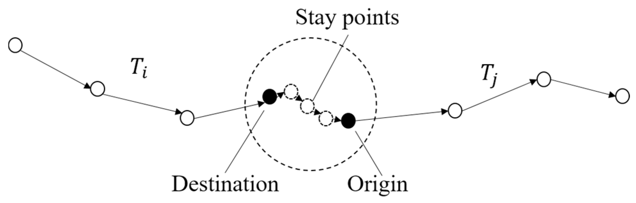
Definition 1.

OD points: OD points of trajectories represent the origin and destination of individual trajectories, including the entrance and exit points of a specific study region and stay points [26].

Definition 2.

Stay points: If the transition duration between adjacent points is greater than a specific threshold while the transition distance is shorter than the distance threshold, these points will be recognized as stay points [37].

Stay points depicted in Figure 2 stand for important geographical locations where moving objects stay for a significant amount of time. Thus, they contain the start and termination of different individual travels. To reduce data redundancy, in the group of stay points, only the endpoints are remained, as depicted in Figure 2.

The distance between two points is given by the Haversine formula:

$$d_{ij}=2R{\sin }^{-1}{({\sin }^2(\frac{la{t}_i-la{t}_j}{2})+\cos (la{t}_i)\cos (la{t}_j){\sin }^2(\frac{lo{n}_i-lo{n}_j}{2}))}^{\frac{1}{2}}$$

(1)

where $d_{ij}$ is the distance between point $i$ and point $j$, $R$ denotes the radius of the earth, $lon$ and $lat$ denote the longitude and latitude of points, respectively. Following the OD points extraction, an individual trajectory is expressed as:

$$T_i=\{P_{iO},P_{i2},\dots ,P_{ij},\dots P_{iD}\}$$

(2)

$$P_{ij}=\{{\mathrm{lon}}_{ij},{\mathrm{lat}}_{ij},{\mathrm{time}}_{ij},{\mathrm{status}}_{ij},\dots \}$$

(3)

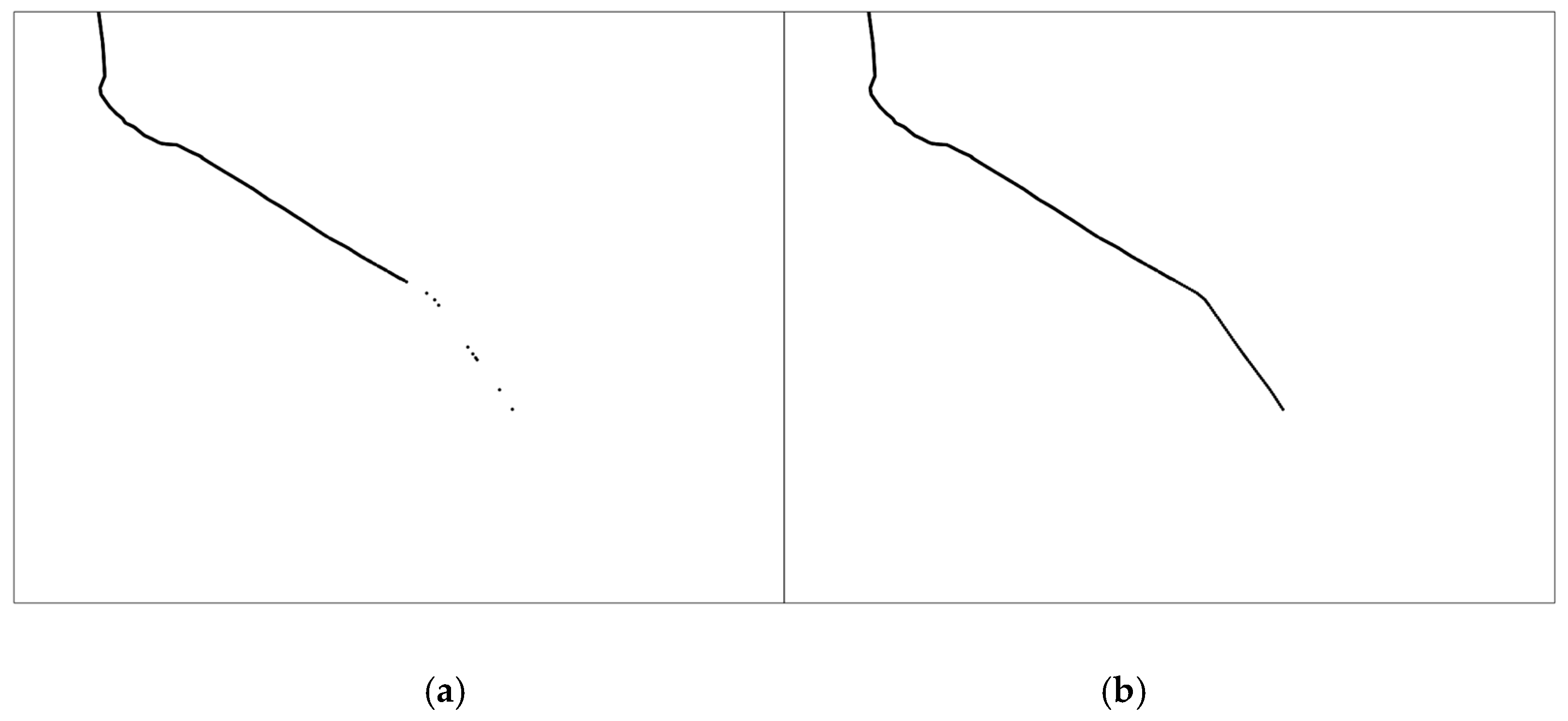
Missing data generated by interruption of the signal or data cleaning could cause information loss, which further lead to poor performance in the following trajectory mining. Thus, it is essential to add interpolation between two points when the interval between them is greater than the predefined threshold. Linear interpolation technique is employed to complement trajectories, as represented in Figure 3. The interval of interpolation is adjustable to guarantee the continuity of trajectory between adjacent grids introduced in the following spatial discretization process.

Characteristics of trajectory will not be expressed sufficiently if it is considered as a one-dimensional time-series and a two-dimensional evenly sampled geometric curve. Thus, we construct a mobility-based structure to represent trajectory. This kind of trajectory structure is three-dimensional containing not only geometrical characteristics, but also geographical and kinematic information. In Reference [33], a certain area just covering each individual trajectory was clipped and discretized. This operation will lose the information on the geographical characteristics and outside the defined area. Instead, we discretize the whole study region into grids, as shown in Figure 4a. Then we define the mobility-based structure of trajectories as follows:

Definition 3.

Mobility-based structure trajectory: The mobility-based structure trajectory refers to an expression of a certain trajectory $T_i$ where $T_i=\{G_{iO},G_{i2},\dots ,G_{ij},\dots G_{iD}\}$. Grid $G_{ij}=\{{\mathrm{m}}_{ij},{\mathrm{n}}_{ij},v_{i,mn}\}$ is a three-dimensional vector, where $m$ and $n$ refer to the row and column index of grids. The third attribute $v_{i,mn}$ is the pixel value of each grid, which present the mobility characteristics of trajectories.

The pixel value $v_{i,mn}$ of each grid shown in Figure 4b is determined as follows:

$$v_{i,mn}=\{\begin{array}{ll}\frac{1}{k}{\displaystyle \sum _j^k}{V}_{ij},& \exists P_{ij}\in T_i{\mathrm{within}\mathrm{grid}}_{mn}\\ 0,& \forall P_{ij}\in T_i{\mathrm{not}\mathrm{in}\mathrm{grid}}_{mn}\end{array}$$

(4)

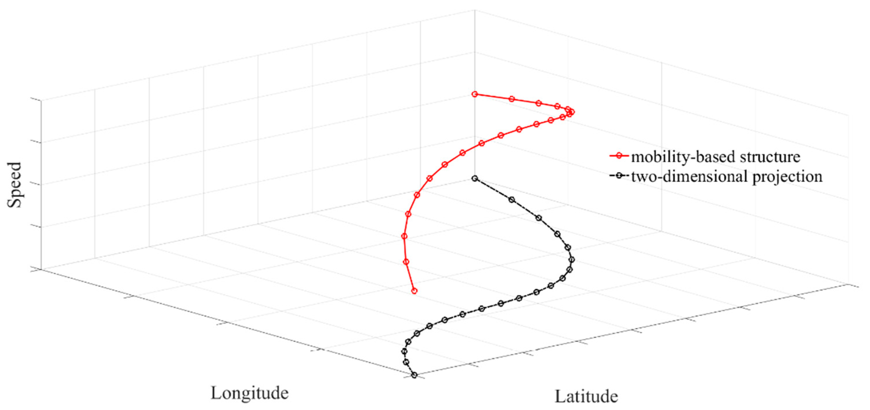
where $k$ denotes the number of points located in ${\mathrm{grid}}_{mn}$, $V_{ij}$ is the speed information of each point $P_{ij}$. Given that the raw speed information provided by devices collection are not reliable enough, $V_{ij}$ is recalculated by the transition duration and distance between adjacent points. Figure 5 presents a schematic diagram of this kind of mobility-based structure trajectory and its projection in a two-dimensional spatial plane. It is three-dimensional comprising three attributes of longitude, latitude, and speed, respectively. The spatial distribution of the non-zero pixels simultaneously reveal the geographical and geometrical characteristics, as well as the moving direction information. Meanwhile, the value of the pixels also reflects the kinematic characteristics of moving objects.

3.2. OD Points Clustering for Route Patterns Discovery

As mentioned in Section 1 and Section 2, the advantages of OD points clustering can be summarized as: (1) the distance function between points is easier to be determined and calculated, and (2) trajectories connecting the same group of origin and destination regions share more similarity and generate more representative frequent route patterns than those that only resemble each other in some partial segments.

The OPTICS algorithm is employed to accomplish points clustering task [20]. The OPTICS algorithm is a density-based algorithm deriving from DBSCAN, which is superior in dealing with the problems of parameter sensitivity and density unbalance [38]. This algorithm generates an order of points which reveals the intrinsic density structure of a points dataset, instead of generating clustering results directly. Subsequently, concrete clustering results can be obtained based on this order. Compared to DBSCAN, which adopts invariable scale parameters to obtain size-fixed clustering results, OPTICS can easily cope with the unbalanced density issue and generate clusters of any size. Euler distance, the most widely used geometric distance function, is calculated by Equation (1) as the similarity measure among points. There are three vital definitions of this method [38]:

Definition 4.

Core-object: Let $x\in X$ be a point in dataset $X$, $\epsilon$ be the distance threshold, $N_{\epsilon }(x)=\left\{x^{\prime }\in X|d(x,x^{\prime })\le \epsilon \right\}$ be the ε-neighborhood of $x$, where $d(x,x^{\prime })$ is the distance between point $x$ and $x^{\prime }$. $x$ is regarded as core-object on condition that $\left|N_{\epsilon }(x)\right|\ge N_{pts}$, where $N_{pts}$ is the point number threshold.

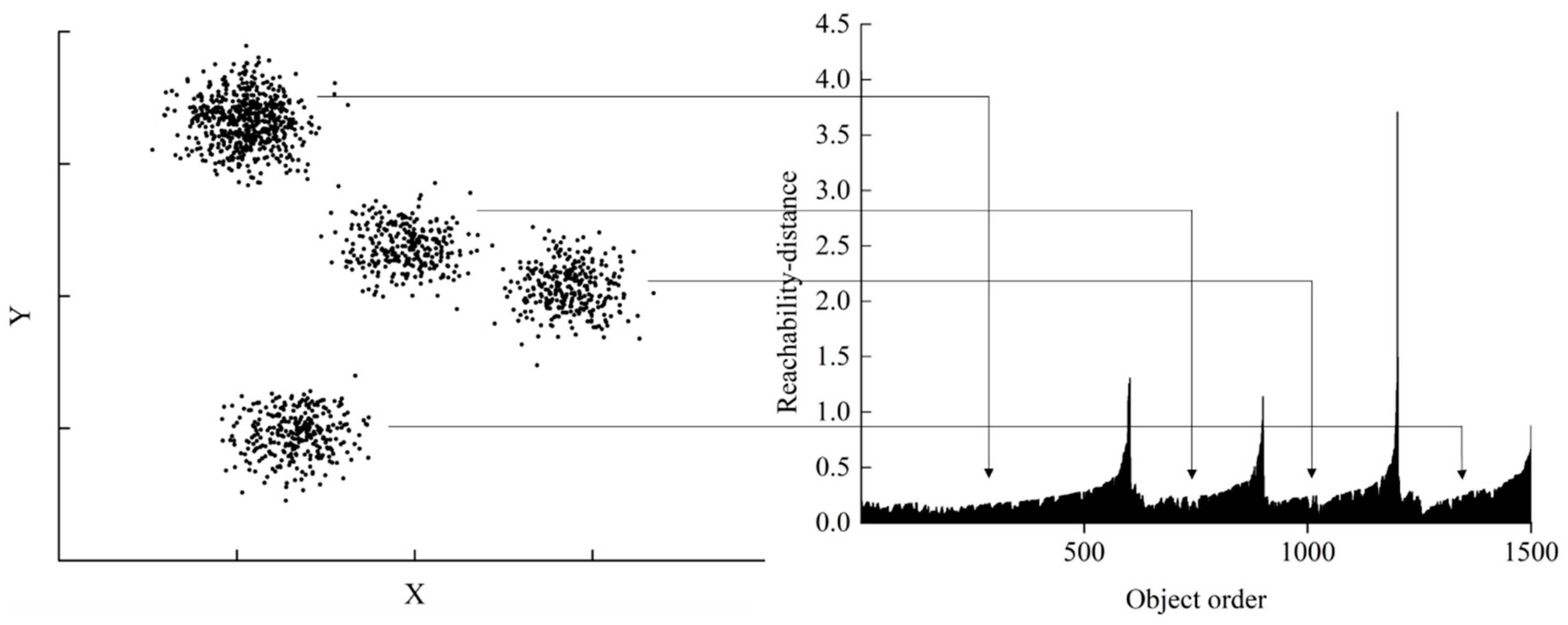
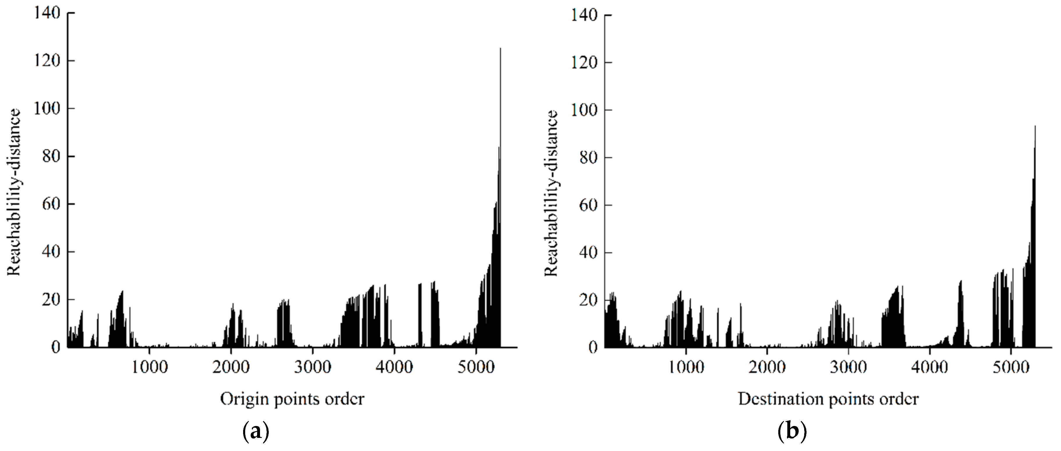
Definition 5.

Core-distance: Core-distance is the smallest distance that makes $x$ become a core-object:

$$cd(x)=\{\begin{array}{ll}undefined,& |N_{\epsilon }(x)|<N_{pts}\\ d(x,N_{\epsilon }^{N_{pts}}(x)),& |N_{\epsilon }(x)|\ge N_{pts}\end{array}$$

(5)

where $N_{\epsilon }^{N_{pts}}(x)$ is the $N_{pts}$-th nearest point to $x$ in the ε-neighborhood set $N_{\epsilon }(x)$. It is remarkable to note that $cd(x)\le \epsilon$.

Definition 6.

Reachability-distance: For both $x,x^{\prime }\in X$, the reachability-distance from $x$ to $x^{\prime }$ is defined as:

$$rd(x^{\prime },x)=\{\begin{array}{ll}undefined,& |N_{\epsilon }(x)|<N_{pts}\\ \max \{cd(x),d(x^{\prime },x)\},& |N_{\epsilon }(x)|\ge N_{pts}\end{array}$$

(6)

The output of the OPTICS algorithm is an order of points with the attributes of core-distance and reachability-distance. Based on this order, reachability-distance of all objects are presented in a reachability plot which intuitively reveals the intrinsic density structure of a dataset, as illustrated in Figure 6. The horizontal axis denotes the objects order and the vertical axis denotes the reachability-distance. The large reachability-distance indicates that this point belongs to a sparse region instead of any possible clusters. On the contrary, a small reachability-distance means a small distance from other points. As a consequence, it is obvious to recognize cluster structures corresponding to the valleys in reachability plot. Clusters with any scale could be obtained automatically from this plot after a concrete steep parameter is determined. This parameter determines the edge of clusters by measuring the variation amplitude of reachability-distance [20].

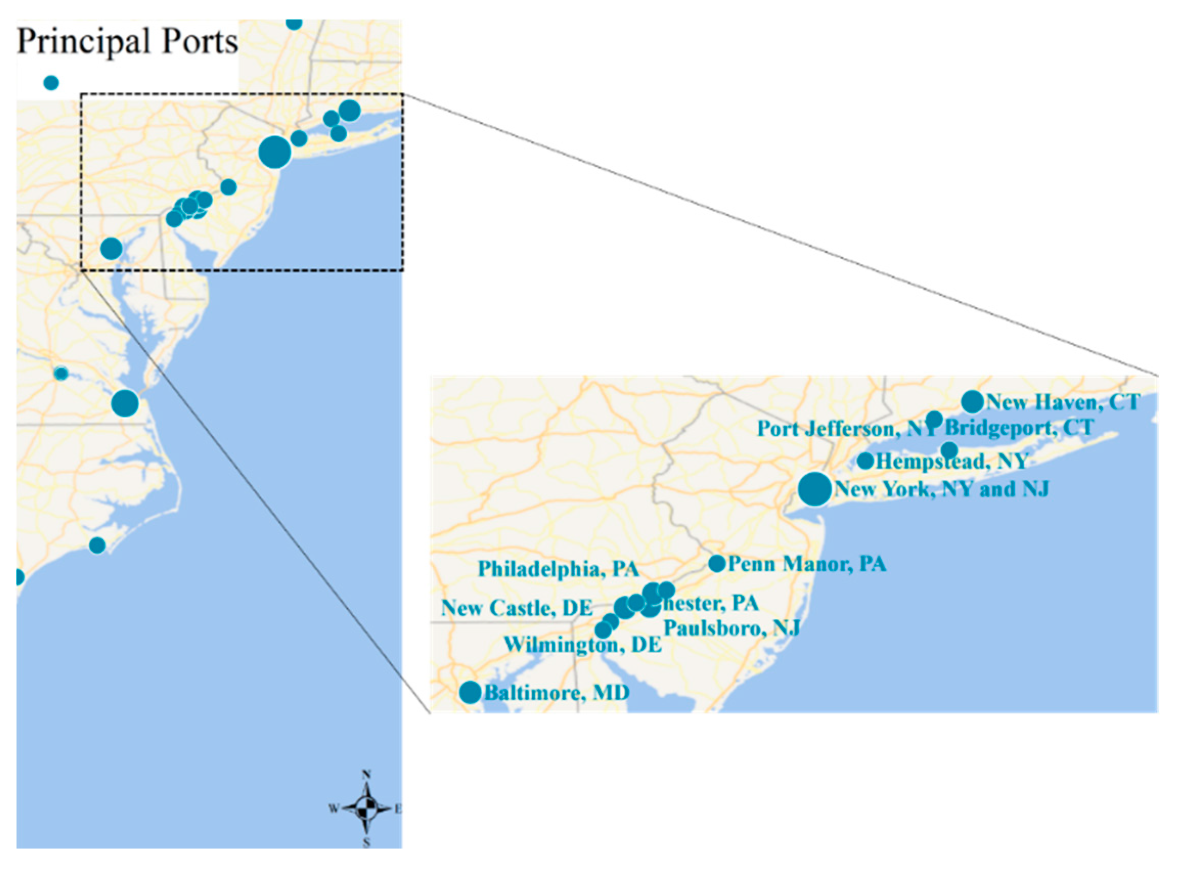
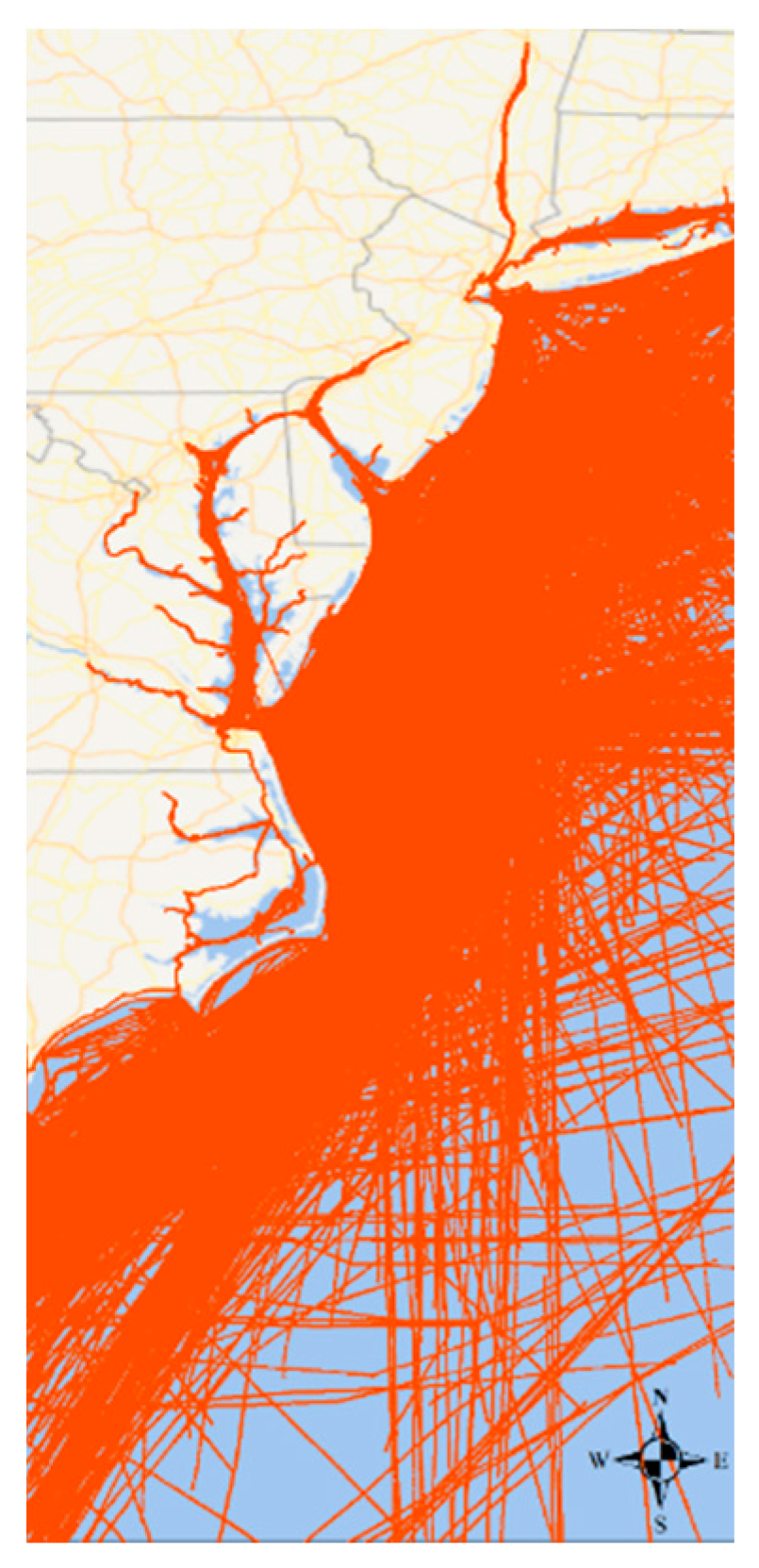
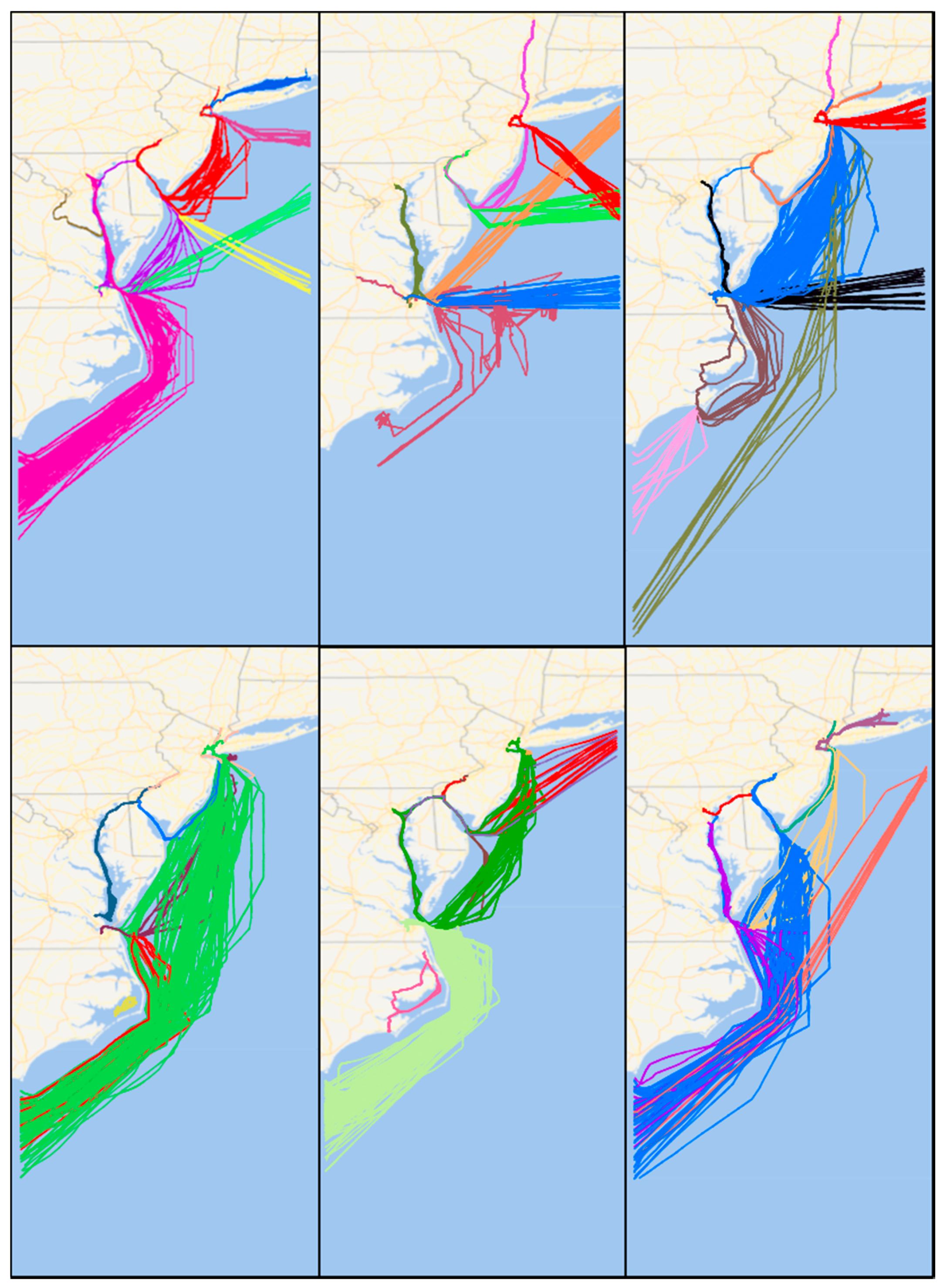
The OD clusters stand for the regions frequently visited by moving objects. They are usually regions of interest ( ROIs ) like shop centers, transportation hubs in city or principal ports in maritime industry. Since plenty of activities emerge in ROIs, there are also a mass of moving objects traveling back and forth among them. Plenty of repeated similar trajectories connecting different ROIs form the active routes (ARs), also called frequent route patterns [39]. Trajectories connecting these ROIs are then picked out to form route patterns after OD points clustering. Additionally, trajectories in the same route pattern also share similar semantic information such as geographical and geometrical characteristics. However, trajectories in active routes connecting the same group of OD clusters may still differ from each other due to the diversity of travel activities. For example, between region A and region B, trajectories of taking the subway are probably different from that of taking taxi. Thus, as explained in Section 1, we take both travel activity types and route patterns into account when investigating mobility modes.

3.3. CNN-Based Method for Mobility Modes Identification

We introduce a mobility modes identification method in a deep learning manner. On the basis of mobility modes discovery method elaborated in Section 3.2, massive history trajectories can be labeled with concrete mobility modes annotation. Then, these trajectories are able to be utilized as training data to train the identification model. The mobility modes identification process consists of two phases: offline model training and real-time identification. Feature extraction and representative learning from trajectory data are crucial issues for training this identification model.

We propose to utilize CNN to accomplish the tasks of feature extraction and identification. Deep features of trajectories, which are recognizable for different mobility modes, can be learned by CNN automatically. The remarkable advantage of CNN compared with ordinary neural network is the character of local connection and weight sharing. In ordinary neural network, every neuron is connected to every neuron in adjacent layers. Instead, neurons in CNN only receive signals from neurons in the local area in the preceding layer. Local connections behave like the receptive field in animals’ brain. This character allows the CNN to capture more local spatial correlations. The weight sharing character in the connection of adjacent layers significantly reduces the number of variables. Both overfitting degree and computation consumption are further alleviated in this way.

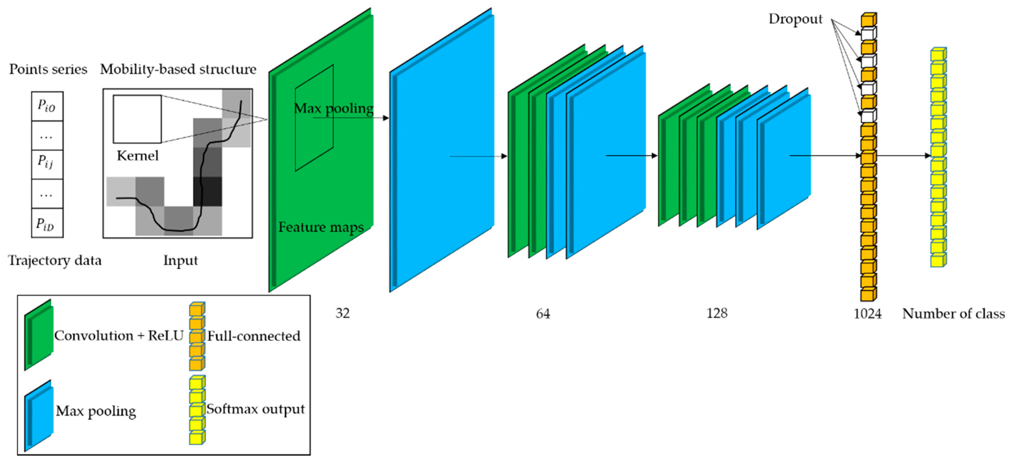
Figure 7 presents the schematic of our proposed identification model. The deep architecture of this model is capable of extracting high-level features from trajectory and also light-weight for training and fine tuning. Trajectory data are transformed into the mobility-based structure described in Section 3.1 and then fed into the CNN. Mobility mode labels of these trajectories are encoded into one-hot vectors and serve as desired output. This identification model is trained through a back-propagation operation. The training process is completed until the optimization process of the objective function converges.

Our CNN architecture was composed of multiple successive layers, as depicted in Figure 7, including: input layer, convolutional layer, pooling layer, fully connected layer, and output layer [16]. The input layer was designed as the mobility-based trajectory structure. The output of each neuron in this layer was equal to the $v_{i,mn}$ attribute of the mobility-based trajectory. Convolutional layers consist of several feature maps. Each feature map connects to the preceding layer via a kernel, i.e., a fixed-size weight matrix. In each iteration, this kernel performs a convolution operation on a group of neighboring neurons within a local area of preceding layer. Then the kernel slid with a fixed stride until this operation was performed on all neurons. After adding a bias to convolution item, the output of convolutional layer was activated by a non-linear activation function like rectified linear unit (ReLU) [34], Sigmoid, tanh, etc. Because of the ability of avoiding a vanishing gradient and the fast converge speed, the ReLU function was chosen to be the activation function in our convolutional layer:

$$y_i=\mathrm{ReLU}(y_{i-1}*W_{i,i-1}+b_i)$$

(7)

$$\mathrm{ReLU}(x)=\{\begin{array}{l}x,x>0\\ 0,x\le 0\end{array}$$

(8)

where $y_{i-1}$ and $y_i$ denote the output of two successive convolutional layers, respectively, $W_{i,i-1}$ denotes the connection weight matrix between them, $*$ represents the operation of convolution, and $b_i$ refers to the bias. Reducing the resolution of the convolutional layer can preserve scale-steady features. Hence, the pooling layer was introduced to carry out down-sample operation after the convolutional layer, as shown in Figure 7. In the pooling layer, down-sample operation aims to derive a unique statistic from the local region of the convolutional layer by taking a pooling strategy. Since the discretization processing was performed on the whole study region, the sparsity problem must be stressed. Therefore, we adopted a max pooling strategy [36] instead of other strategies since it always performs well in the process of separating sparse features. The pooling layer also alleviates the computational burden due to the reduction of variables. Moreover, the function of a fully connected layer includes: (1) converting the stimulation signal from hidden convolutional layers into one-dimensional form for the output layer, and (2) extracting higher-level features. Ultimately, the output layer generates a probability distribution over the classification labels by resorting to logistic regression function Softmax:

$$\mathrm{Softmax}(x_i)=\frac{\exp (x_i)}{{\displaystyle \sum _j^X\exp (x_j)}}$$

(9)

where $X$ is a set including all the received stimulation $x_i$ of the output layer.

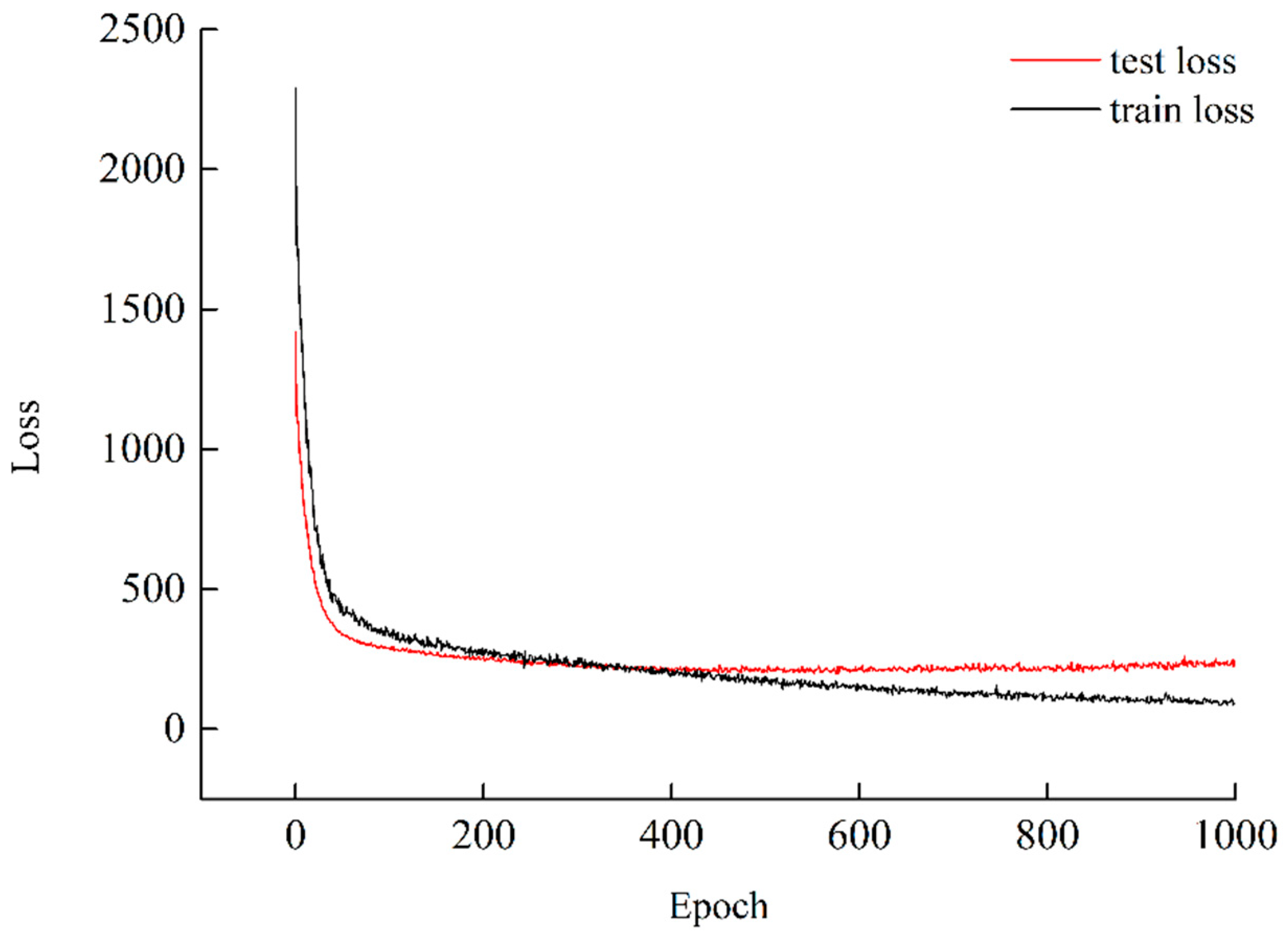
Limited by the volume of the dataset and the complexity of the CNN architecture, overfitting was an inevitable issue of our model. Overfitting means the trained identification model is short of generalization ability. Thus, we introduced L2 regularization [36] and the dropout technique [35] to deal with this issue. The prediction error between the actual output and desired output is called loss function. Loss function is the objective function decreased in the back-propagation process of each iteration by means of gradient descend optimizer such as adaptive moment estimation (Adam) optimizer [40]. However, this operation may produce large weights and further leads to instability of prediction results. The L2 regularization aims to add the quadratic sum of weights to loss function. There is a tradeoff between the decrease of weights and prediction error in loss function after adding L2 regularization. Cross-entropy function with L2 regularization was chosen to be the objective function in the training process:

$$\begin{array}{ll}los{s}_{reg}& =los{s}_{unreg}+\lambda {\Vert W\Vert }_2^2\\ & =-{\displaystyle \sum _x[y\ln {\mathrm{y}}^{\prime }+(1-\mathrm{y})ln(1-{\mathrm{y}}^{\prime })]}+\lambda {\Vert W\Vert }_2^2\end{array}$$

(10)

where $los{s}_{reg}$ and $los{s}_{unreg}$ denote the loss function with and without L2 regularization, respectively. In Equation (10), $los{s}_{unreg}$ is calculated by cross-entropy function where $x$ is the input, $y$ and $y^{\prime }$ are the desired output and actual output, respectively.$\lambda$ is the weight decay parameter measuring the proportion of regularization item in loss function, ${\Vert W\Vert }_2^2$ refers to the quadratic sum of all weight variables in Equation (7). Dropout technique stochastically removes a portion of hidden neurons with a certain probability, as shown in Figure 7. In this way, different architecture is trained in each iteration of the training process. Dropout alleviates the complexity and co-adaption of neurons and consequently enhances the generalization ability of our identification model.

4. Experimental Results

In this section, the proposed method is applied to real-world trajectory data. Section 4.1 presents a brief description of the dataset. The mobility modes are discovered based on the extraction of latent route patterns in Section 4.2. In Section 4.3, the configuration details of mobility modes identification model are elaborated. The performance of this model is also evaluated and compared with some widely used approaches. To present an intuitionistic understanding about the process of identification, the deep features learned by our model are visualized in Section 4.4.

4.1. Data Description

Trajectory data employed in our work were AIS data obtained from MarineCadastre.gov [41] which provides vessel traffic data records for US coastal waters. The AIS data contain two types of data: static data and dynamic data [20]. Static data contain information about vessels including ship name, Maritime Mobile Service Identity (MMSI), ship type, ship size, etc. The MMSI is the unique identity of an individual vessel. Dynamic data contain information collected by various sensors during the travel process, including location and time information obtained by GNSS (Global Navigation Satellite System), SOG (Speed over Ground), COG (Course over Ground) and Heading, etc.

The study region was the east coastal region of the US (from N 30.1° to N 42.8° and W 72° to W 78°). This is one of the busiest shipping regions in the world with a group of principal ports, as shown in Figure 8. The dataset covered historical records in four consecutive months from 1 May to 31 August 2014. In order to guarantee that sufficient information was retained in trajectories, each single voyage selected contained at least 500 messages. After the data cleaning process, more than 5000 useful voyages were retained for subsequent investigation, as delineated in Figure 9. The static data provided the distribution information of travel activities, as presented in Figure 10. The combinations of activity types and route patterns constituted different mobility modes.

4.2. Route Patterns Discovery

It is difficult to recognize route patterns and set apart any main shipping lanes from the whole trajectory dataset artificially, as delineated in Figure 9. However, the OD points clustering approach is capable of coping with this issue. After the performance comparison among repeated experiments, the parameters of OPTICS were configured as follows:$Minpts$, the minimum number of points to form a cluster, was set to 5. To obtain the ultimate clustering result from the reachability plot, steep parameter $\xi$ that determines the edge of clusters was set to 0.2.

Figure 11 depicts the reachability plots of origin and destination point sets. It explicitly uncovers the intrinsic density structure of OD points. Subsequently, clusters with different density and different scale were picked out based on these plots. Trajectories of voyages that depart from or head to different groups of OD clusters were picked out to generate different route patterns, which are presented by different colors in Figure 12. It is straightforward to observe that the spatial distribution of some OD clusters was in accordance with the location of principal ports, indicating the reliability of the clustering result. These trajectories establish the connection among ROIs including principal ports, gateways to the great ocean, and main operation areas. These route patterns can be categorized into three groups in terms of the semantic meaning of the corresponding OD clusters. The first one is domestic routes, the trajectories of which are complete among the principal ports, and main operation areas within the study region. The second one contains trajectories connecting the principal ports and gateways to the great ocean. Additionally, the third kind of route patterns just pass by the study region via gateways to the great ocean.

Route patterns reveal both the distribution of ARs that represent the main shipping lanes and the location of ROIs including the principal ports, gateways to the great ocean, and the main operation areas. For instance, the uncovered route patterns presented in Figure 13a,b behave irregularly and distinctively. According to the travel activity information from static data, these two route patterns are generated by fishing and law enforcement activities, respectively. In consequence, the clustering result provides valuable clues about the location of significant sea areas where plenty of specific vessel travel activities concentrate and unexpected accidents could potentially emerge. This approach is expected to be applied to frequent route patterns extraction and abnormal events prevention in transportation management and maritime traffic surveillance.

Although most route patterns demonstrated above are regular and distinguishable from each other, some of them are still not compact enough and behave disorderly, such as the one shown in Figure 13c. It is intuitive to attribute this phenomenon to the travel activity type diversity. For instance, according to the static data, the route patterns illustrated in Figure 13c are mostly generated by the tugging activity. Tugs always maneuver vessels and other objects like oil platforms by pushing or tugging them at any possible sea area, and as a consequence, the trajectories seem like arbitrary behavior. In addition, there also exists discrepancy among trajectories which belong to the same route pattern but are generated by different travel activities. Hence, it is insufficient to investigate mobility behavior without considering the travel activity information. In the aforementioned definition of mobility modes, knowledge of both the route patterns and travel activity types are taken into account. In the analysis of AIS data, massive history vessel trajectory data are categorized into different mobility modes in the form of: a vessel from New York, NY and NJ to Philadelphia, PA for carrying cargo.

4.3. Mobility Modes Identification

In the process of training the mobility modes identification model, history trajectory was transformed into the mobility-based structure introduced above. Each one of them was labeled with an annotation containing the mobility modes information. These semantic labels were encoded into one-hot vectors to serve as the desired output and ground truth. We adopted ten-fold cross validation strategy on the whole dataset. The whole dataset was divided into ten subsets. For each experiment, one of them served as test data and the rest were training data. Then this experiment was repeated ten times until all of the data had been treated as test data.

We employed a manual search strategy inspired by Reference [42] in the training process to determine the optimal hyper-parameter and layer configuration of CNN architecture.

Table 1. Configuration of the CNN architecture.

Layers or Parameters	Concrete Configuration
Hidden convolutional layer	3 layers (ReLU)
Hidden pooling layer	3 layers (max pooling)
Fully connected layer	1 layer (ReLU)
Output layer	Softmax
Optimizer	Adam
Initial learning rate	0.1
Loss function	Cross entropy
Regularization	L2 ($\lambda$ = 0.1)
Dropout probability	0.9 (only in fully connected layer)

presents the ultimately determined parameters and the configuration details of our model. There was only one channel in the input layer, which carried the information of $v_{i,mn}$, the third attribute of three-dimensional mobility-based structure trajectory. The number of channels in three hidden convolutional layers, i.e., the feature maps in Figure 7, increases successively like a pyramid, which are 32, 64, and 128. The max pooling strategy was adopted due to its high efficiency in the process of separating the sparse features compared with other strategies like mean pooling. Dropout operation was only implemented in the fully connected layer. It was unnecessary to drop out neurons in the convolutional layers since the number of variables in these layers was small enough. The Softmax function was utilized as the classification function in the output layer to generate the final identification result, since it performs well in computing class scores. The training of the identification model was completed offline since it is time-consuming and built on history trajectory data. Once the training process was completed, the identification task could be accomplished in a real-time manner.

In order to evaluate our proposed method intuitively, two kinds of comparative experiments were involved. Firstly, we intended to evaluate our proposed mobility-based trajectory structure. Another trajectory structure with only two-dimensional spatial information was introduced to serve as the input of the designed identification model. This kind of structure was similar to our proposed one, but the pixel value of it was equal to the sample number. This comparison group was named 2D+CNN due to this trajectory structure only conveying two-dimensional information. Then, in order to assess the learning efficiency of our designed CNN architecture comparatively, several widely used machine learning algorithms were introduced to deal with the proposed mobility-based trajectory. These experiments involve the support vector machine (SVM), decision tree (DT), and random forest (RF)-based methods [1], which are named MB+SVM (mobility-based trajectory structure + SVM), MB+DT, and MB+RF, respectively. The optimal hyper-parameters of these machine learning algorithms were determined by grid search strategy. We also introduce the optimal CNN architecture proposed in Reference [16] as a comparative experiment, named as MB+CNN [16]. The CNN architecture utilized in Reference [16] is deeper and more complicated than that of this paper. Additionally, the proposed method of this work was named MB+CNN. The overall performance of these methods was evaluated by the average result of ten-fold cross validation.

Due to the number of trajectories contained in different mobility modes being imbalanced, accuracy was not the only criterion we focus on. We introduce several evaluation criterions for evaluation, including accuracy, precision, recall, F1-score, and area under curve (AUC). Accordingly, a detailed performance evaluation is set out in

Table 2. Comparative performance evaluation of proposed method and other methods. MB+CNN: mobility-based trajectory structure with convolutional neural network proposed in this work, 2D+CNN: two-dimensional trajectory with convolutional neural network proposed in this work, MB+SVM: mobility-based trajectory structure with support vector machine, MB+DT: mobility-based trajectory structure with decision tree, MB+RF: mobility-based trajectory structure with random forest, MB+CNN [16]: mobility-based trajectory structure with convolutional neural network proposed in [16].

Groups	Accuracy	Precision	Recall	F1-score	AUC
MB+CNN	0.858	0.861	0.858	0.847	0.997
2D+CNN	0.821	0.822	0.821	0.811	0.993
MB+SVM	0.797	0.799	0.797	0.78	0.996
MB+DT	0.667	0.711	0.667	0.671	0.831
MB+RF	0.752	0.734	0.752	0.724	0.993
MB+CNN [16]	0.826	0.831	0.826	0.819	0.996

. The AUC in the last column refers to the area under receiver operating characteristic (ROC) curve. The ROCs illustrated in Figure 14 evaluate the efficiency of methods when distinguishing different modes. The prediction result will be proved to be almost random speculation if the ROC is close to the straight dash line, i.e., AUC was equal to 0.5. On the contrary, AUC is always expected to be close to 1.

According to Table 2, our proposed method yields the best result in all concerned metrics as expected. The prediction accuracy of the two groups which our CNN architecture was involved in designing were 85.8% and 82.1%, respectively. Whereas the accuracy of other machine learning algorithms was lower than 80%. The SVM yields the best result among three machine learning algorithms. The RF, which is the ensemble of DT, also achieved better performance than DT. Our CNN architecture led to significant improvement in accuracy which is higher than 6.1 % compared to the best performance of other machine learning algorithms. Our method also achieved 3.2% higher accuracy than the CNN utilized in Reference [16], since the depth and complexity of the network architecture may reduce the performance. The mobility-based structure of trajectory also led to a 3.7% improvement in accuracy compared to the 2D-CNN group. The F1-score is the balanced score of precision and recall, which presents intuitional measure when both these two metrics are expected to be high. The F1-score yielded by our proposed method was 84.7%, which is prominent compared to the highest F1-score 81.9% of other comparative methods. The highest AUC was also achieved by the MB+CNN group. The combinations of several route patterns and eight types of known travel activities make up dozens of mobility modes. Hence, the results of our method were sufficient for identification tasks when faced with mobility modes diversity. In addition, the identification performance also confirms the reliability of the mobility modes discovery results in Section 4.2, since the identification performance will be very poor if the labeled data are chaotic and undistinguishable.

Figure 15 depicts the training process of our model. We evaluate the identification performance on test dataset after every training epoch. The loss function descending process on test dataset converged in the vicinity of 500th epoch. The performance did not become poor with the training process advancing forward. Hence this process strongly proves the good character of the configuration of our designed CNN architecture. It avoids the problems of both underfitting and overfitting so that it is easy to be generalized to more trajectory data.

4.4. Deep Features Visualization

The visualization of extracted deep features is helpful for comprehending the inherent mechanism of trained identification model. We conducted gradients calculation to visualize deep features extracted by hidden convolutional layers. The gradients were calculated by partial derivative as follows:

$$\nabla F^h(\mathrm{m},\mathrm{n})=\frac{\partial F^h}{\partial v_{m\mathrm{n}}}$$

(11)

where $F^h$ denotes the output feature of the $h$-th hidden layer, and $v_{m\mathrm{n}}$ is the pixel value of ${\mathrm{grid}}_{mn}$ in the input layer. The gradients between the hidden layers and the input layer reflect the contribution of input signals on deep features in hidden layers.

Figure 16 depicts the deep features captured by three hidden convolutional layers in the identification process of two trajectories of different mobility modes. These two trajectories are similar in geographical and geometrical characteristics but generated by different travel activities of cargo and tanker respectively. The dark degree of the color indicates the contribution from the input layer. Obviously, with the embedding of deeper layers, the features learned by our model become more abstractive. According to Figure 16, the first stage of the convolution process mainly focuses on the macroscale features such as the edge shape of the trajectory curve. These macroscale features are distinguishable for recognizing mobility modes in different route patterns. The following convolutional layer learns more microscale features further. More distinguishable details such as the inflection corners are captured by this deeper layer. From the last convolutional layer, it is noticeable that the areas in the vicinity of origin and destination are much more recognizable. These deep features are crucial for obtaining the accurate identification result. These two trajectories are easily-confused due to the sharing of the same origin and destination regions. However, different features are still captured by our identification model. Even though it is still difficult to artificially interpret after visualization. The well-trained model is capable of recognizing the meaning of these abstractive features well.

5. Discussion and Conclusions

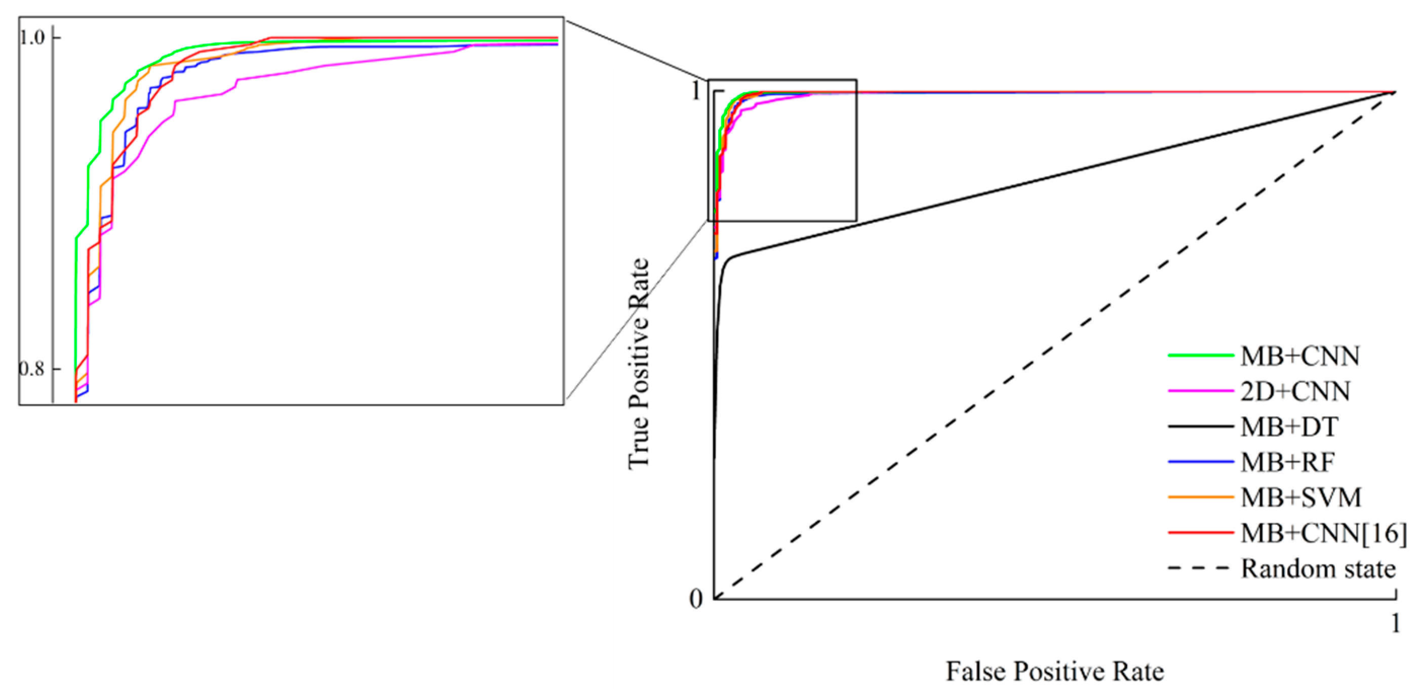
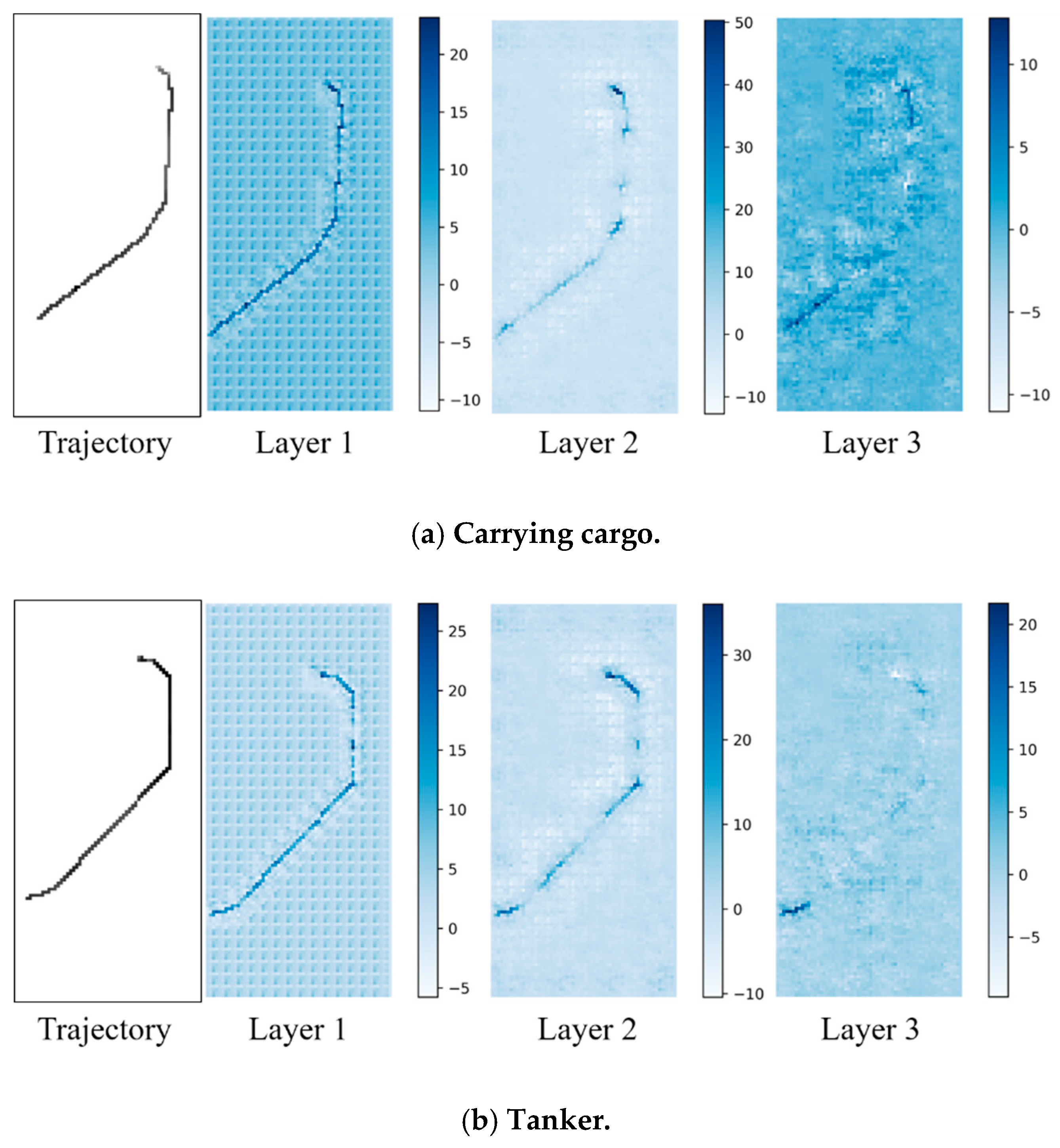
In this work, we proposed a data-driven method to mine the potential knowledge about mobility modes from raw trajectory data. The concerned issues consisted of two aspects: (1) mobility modes discovery and (2) mobility modes identification. Our method aimed to integrate these two issues together. To achieve this goal, we presented an unsupervised approach, i.e., OD points clustering, to discover route patterns from massive history trajectories. Then, we built a CNN-based identification model by taking advantage of the labeled history trajectory data. Experimental results on real data indicate the reasonable superiority of our method as expected. Further, visualization of deep features was also inspiring for understanding the mechanism of deep learning.

The conclusion of this work can be summarized as follows. (1) In the phase of mobility modes discovery, the proposed OD points clustering method performed excellently in discovering different route patterns. The uncovered mobility modes containing abundant geographical and semantic information were useful knowledge hidden in massive history trajectory data. This method and the corresponding results were valuable for land use planning and traffic management. (2) We put forward an advanced mobility-based structure of trajectory which integrated geometrical, geographical, and kinematic information comprehensively. This well-designed structure is preferable for capturing representative features directly from trajectories. (3) Moreover, we proposed a deep learning model leveraging a CNN to identify mobility modes. This model achieved good performance in capturing the deep features without any domain knowledge. This approach could be used to provide real-time identification result for traffic surveillance.

This work presents a typical way to transform the raw trajectory data into knowledge and decision support. This way is expected to be applied to many other trajectory mining investigation and various practical application fields. There still exist future fields to be explored over this work. Firstly, we will try to synthesize more useful attributes to construct a multi-dimensional trajectory structure, such as semantic and temporal information. We believe that more knowledge contained in multi-attributes can make different mobility modes more recognizable. In addition, we plan to perform further study on routes and destination prediction and abnormal behavior detection based on mobility modes awareness.