Spatial Interaction Modeling of OD Flow Data: Comparing Geographically Weighted Negative Binomial Regression (GWNBR) and OLS (GWOLSR)


Abstract
:1. Introduction
2. Materials and Methods
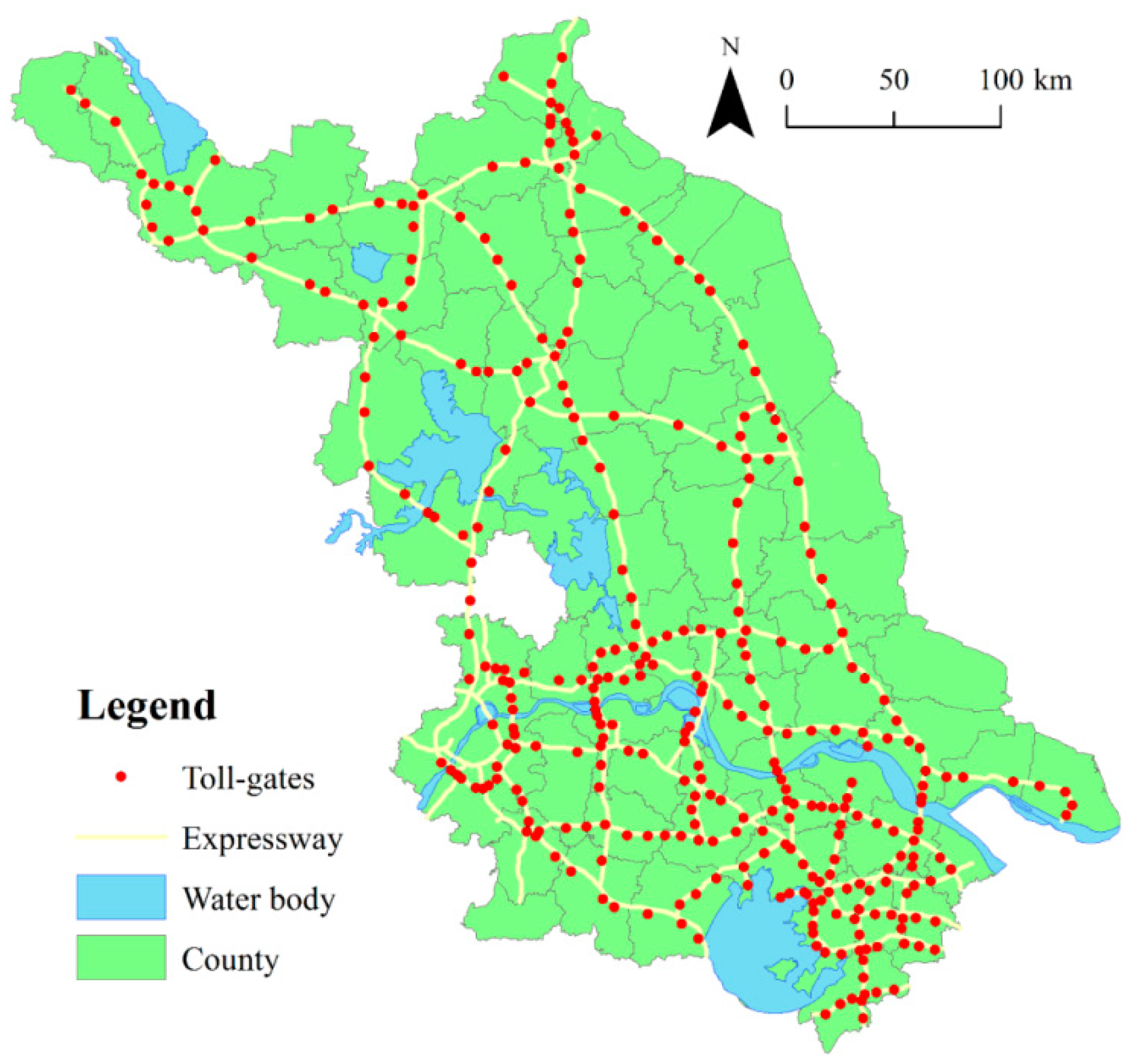
2.1. Study Area
2.2. Data Collection
2.3. Global and Local Modeling
2.3.1. Global Models of Flow
2.3.2. Local Models of Flow
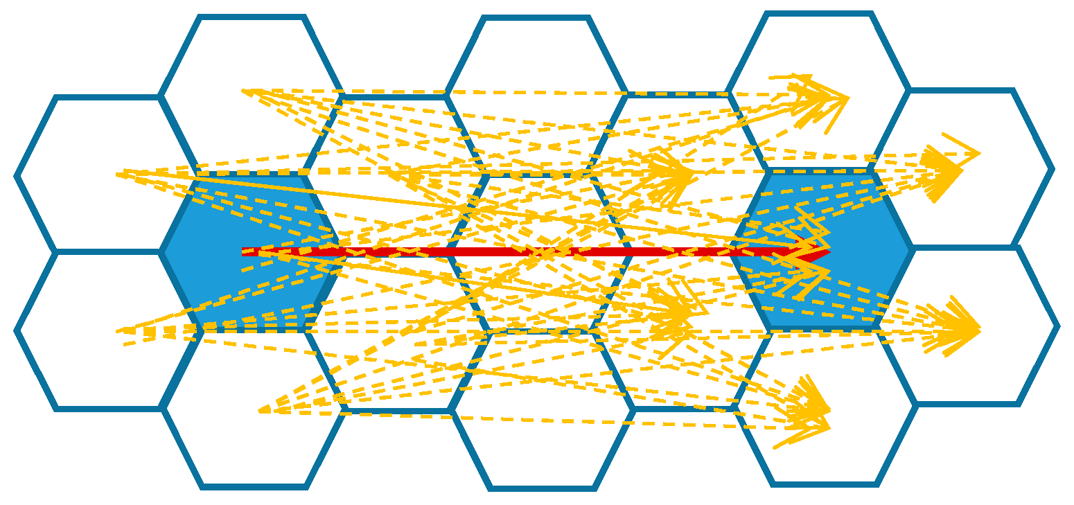
2.3.3. Bandwidth
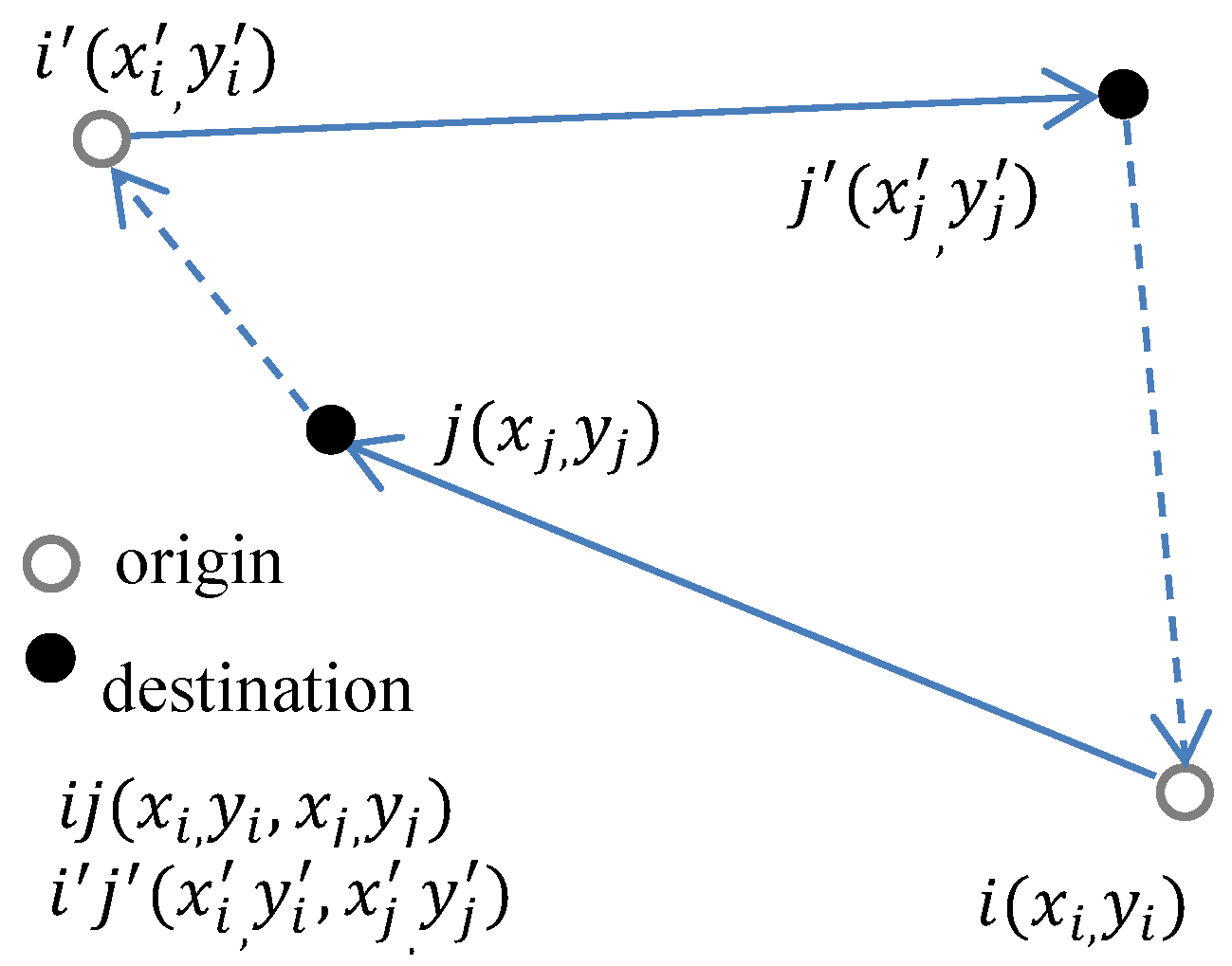
2.3.4. Flow-Based Global Moran
2.3.5. Comparisons
3. Results
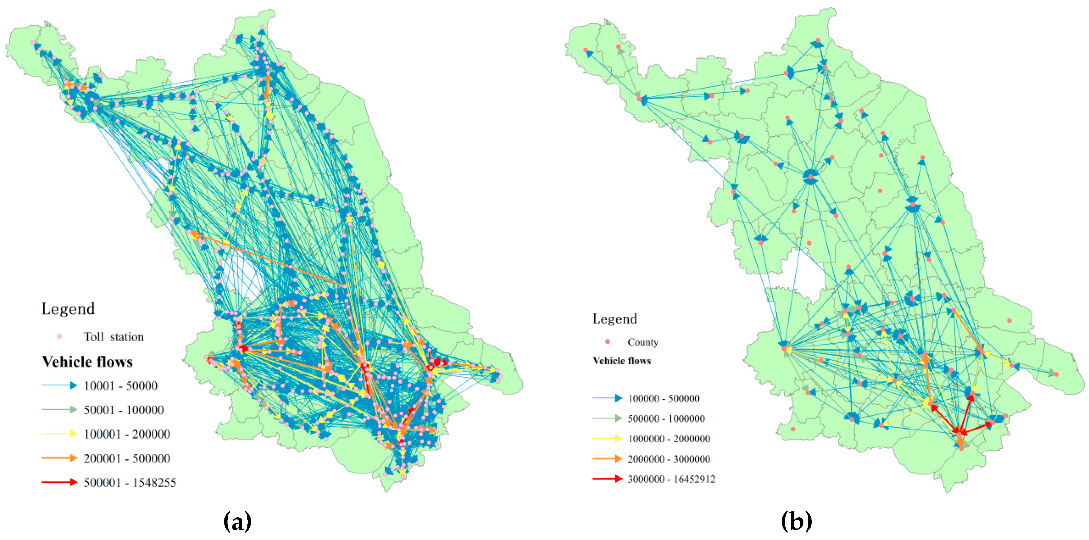
3.1. Flow Patterns
3.2. Global Modeling—OLS/NB
3.3. Local Modeling—OLS/NB
3.3.1. GWOLS Flowing Model
3.3.2. GWNBR Flowing Model
4. Discussion
5. Conclusions
Author Contributions
Funding
Conflicts of Interest
References
- Cheng, J.; Young, C.; Zhang, X.; Owusu, K. Comparing inter-migration within the European Union and China: An initial exploration. Migr. Stud. 2014, 2, 340–368. [Google Scholar] [CrossRef] [Green Version]
- Mak, J.; Moncur, J.E. Interstate migration of college freshmen. Ann. Reg. Sci. 2003, 37, 603–612. [Google Scholar] [CrossRef]
- Hwang, C.C.; Shiao, G.C. Analyzing air cargo flows of international routes: An empirical study of Taiwan Taoyuan International Airport. J. Transp. Geogr. 2011, 19, 738–744. [Google Scholar] [CrossRef]
- Neumayer, E. On the detrimental impact of visa restrictions on bilateral trade and foreign direct investment. Appl. Geogr. 2011, 31, 901–907. [Google Scholar] [CrossRef] [Green Version]
- McArthur, D.P.; Kleppe, G.; Thorsen, I.; Ubøe, J. The spatial transferability of parameters in a gravity model of commuting flows. J. Transp. Geogr. 2011, 19, 596–605. [Google Scholar] [CrossRef] [Green Version]
- Jin, C.; Cheng, J.; Xu, J. Using user-generated content to explore the temporal heterogeneity in tourist mobility. J. Travel Res. 2018, 57, 779–791. [Google Scholar] [CrossRef]
- Hoffmann, V.H.; Sprengel, D.C.; Ziegler, A.; Kolb, M.; Abegg, B. Determinants of corporate adaptation to climate change in winter tourism: An econometric analysis. Glob. Environ. Chang. 2009, 19, 256–264. [Google Scholar] [CrossRef]
- Fotheringham, A.S.; Brunsdon, C.; Charlton, M. Geographically Weighted Regression: The Analysis of Spatially Varying Relationships; Wiley: Chichester, UK, 2002; pp. 53–142. [Google Scholar]
- Xia, F.; Rahim, A.; Kong, X.; Wang, M.; Cai, Y.; Wang, J. Modeling and Analysis of Large-Scale Urban Mobility for Green Transportation. IEEE Trans. Ind. Inform. 2018, 14, 1469–1481. [Google Scholar] [CrossRef]
- Liao, C.; Brown, D.; Fei, D.; Long, X.; Chen, D.; Che, S. Big data-enabled social sensing in spatial analysis: Potentials and pitfalls. Trans. GIS 2018, 22, 1351–1371. [Google Scholar] [CrossRef]
- Long, Y.; Thill, J.C. Combining smart card data and household travel survey to analyze jobs-housing relationships in Beijing. Comput. Environ. Urban. 2015, 53, 19–35. [Google Scholar] [CrossRef]
- Zhang, Z.; He, Q.; Tong, H.; Gou, J.; Li, X. Spatial-temporal traffic flow pattern identification and anomaly detection with dictionary-based compression theory in a large-scale urban network. Transp. Res. Part C 2016, 71, 284–302. [Google Scholar] [CrossRef]
- Jenelius, E. Network structure and travel patterns: Explaining the geographical disparities of road network vulnerability. J. Transp. Geogr. 2009, 17, 234–244. [Google Scholar] [CrossRef]
- Kim, J.; Mahmassani, H.S. Spatial and temporal characterization of travel patterns in a traffic network using vehicle trajectories. Transp. Res. Procedia 2015, 9, 164–184. [Google Scholar] [CrossRef]
- Wilson, A.G. A family of spatial interaction models, and associated developments. Environ. Plan. A 1971, 3, 1–32. [Google Scholar] [CrossRef]
- Roy, J.R.; Thill, J.C. Spatial interaction modeling. Pap. Reg. Sci. 2004, 83, 339–361. [Google Scholar] [CrossRef]
- Qian, Z.S.; Li, J.; Li, X.; Zhang, M.; Wang, H. Modeling heterogeneous traffic flow: A pragmatic approach. Transp. Res. Part B 2017, 99, 183–204. [Google Scholar] [CrossRef]
- Hui, M.; Bai, L.; Li, Y.; Wu, Q. Highway traffic flow nonlinear character analysis and prediction. Math. Probl. Eng. 2015, 2015, 902191. [Google Scholar] [CrossRef]
- Manley, E.; Cheng, T. Exploring the role of spatial cognition in predicting urban traffic flow through agent-based modeling. Transp. Res. Part A 2015, 109, 14–23. [Google Scholar]
- Ahn, J.; Ko, E.; Kim, E.Y. Highway traffic flow prediction using support vector regression and Bayesian classifier. In Proceedings of the 2016 International Conference on Big Data and Smart Computing (BigComp), Hong Kong, China, 18–20 January 2016; pp. 239–244. [Google Scholar]
- Lv, Y.; Duan, Y.; Kang, W.; Li, Z.; Wang, F.Y. Traffic flow prediction with big data: A deep learning approach. IEEE Trans. Intell. Transp. 2015, 16, 865–873. [Google Scholar] [CrossRef]
- Jung, W.S.; Wang, F.; Stanley, H.E. Gravity model in the Korean highway. EPL (Europhys. Lett.) 2008, 81, 48005. [Google Scholar] [CrossRef] [Green Version]
- Chen, W.; Liu, W.; Ke, W.; Wang, N. Understanding spatial structures and organizational patterns of city networks in China: A highway passenger flow perspective. J. Geogr. Sci. 2018, 28, 477–494. [Google Scholar] [CrossRef]
- Fischer, M.M.; Griffith, D.A. Modelling spatial autocorrelation in spatial interaction data. J. Reg. Sci. 2008, 48, 969–989. [Google Scholar] [CrossRef]
- LeSage, J.P.; Pace, R.K. Spatial econometric modeling of origin-destination flows. J. Reg. Sci. 2008, 48, 941–967. [Google Scholar] [CrossRef]
- Chun, Y.; Kim, H.; Kim, C. Modeling interregional commodity flows with incorporating network autocorrelation in spatial interaction models: An application of the US interstate commodity flows. Comput. Environ. Urban 2012, 36, 583–591. [Google Scholar] [CrossRef]
- Kordi, M.; Fotheringham, A.S. Spatially Weighted Interaction Models (SWIM). Ann. Am. Assoc. Geogr. 2016, 106, 990–1012. [Google Scholar] [CrossRef]
- Lloyd, C.D. Local Models for Spatial Analysis; CRC Press: Boca Raton, FL, USA, 2010; pp. 97–123. [Google Scholar]
- Trigg, D.W.; Leach, A.G. Exponential smoothing with an adaptive response rate. J. Oper. Res. Soc. 1967, 18, 53–59. [Google Scholar] [CrossRef]
- Foster, S.A.; Gorr, W.L. An adaptive filter for estimating spatially-varying parameters: Application to modeling police hours spent in response to calls for service. Manag. Sci. 1986, 32, 878–889. [Google Scholar] [CrossRef]
- Hadayeghi, A.; Shalaby, A.; Persaud, B. Development of planning-level transportation safety models using full Bayesian semiparametric additive techniques. J. Transp. Saf. Secur. 2010, 2, 45–68. [Google Scholar] [CrossRef]
- Da Silva, A.R.; Rodrigues, T.C.V. Geographically weighted negative binomial regression-incorporating overdispersio. Stat. Comput. 2014, 24, 769–783. [Google Scholar]
- Jin, C.; Cheng, J.; Xu, J.; Huang, Z. Self-driving tourism induced carbon emission flows and its determinants in well-developed regions: A case study of Jiangsu province, China. J. Clean. Prod. 2018, 186, 191–202. [Google Scholar] [CrossRef]
- Wei, Y.D. Beyond new regionalism, beyond global production networks: Remaking the Sunan Model, China. Environ. Plan. C 2010, 28, 72–96. [Google Scholar] [CrossRef]
- Jiangsu Bureau of Statistics (JBS). Jiangsu Statistical Yearbook 2014; China Statistical Press: Beijing, China, 2015; pp. 1–199. [Google Scholar]
- Bröcker, J.; Korzhenevych, A.; Schürmann, C. Assessing spatial equity and efficiency impacts of transport infrastructure projects. Transp. Res. Part B 2010, 44, 795–811. [Google Scholar] [CrossRef]
- Han, J.; Hayashi, Y. Assessment of private car stock and its environmental impacts in China from 2000 to 2020. Transp. Res. Part D Transp. Environ. 2008, 13, 471–478. [Google Scholar] [CrossRef]
- Krisztin, T.; Fischer, M.M. The gravity model for international trade: Specification and estimation issues. Spat. Econ. Anal. 2015, 10, 451–470. [Google Scholar] [CrossRef]
- Etzo, I. The determinants of the recent interregional migration flows in Italy: A panel data analysis. J. Reg. Sci. 2011, 51, 948–966. [Google Scholar] [CrossRef]
- Khadaroo, J.; Seetanah, B. The role of transport infrastructure in international tourism development: A gravity model approach. Tour. Manag. 2008, 29, 831–840. [Google Scholar] [CrossRef]
- Matsumoto, H. International urban systems and air passenger and cargo flows: Some calculations. J. Air Transp. Manag. 2004, 10, 239–247. [Google Scholar] [CrossRef]
- Fotheringham, A.S.; O’Kelly, M.E. Spatial Interaction Models: Formulations and Applications; Kluwer Academic Publishers: Dordrecht, The Netherlands, 1989; pp. 65–156. [Google Scholar]
- Kimura, F.; Lee, H.H. The gravity equation in international trade in services. Rev. World Econ. 2006, 142, 92–121. [Google Scholar] [CrossRef]
- Piras, R. A long-run analysis of push and pull factors of internal migration in Italy. Estimation of a gravity model with human capital using homogeneous and heterogeneous approaches. Pap. Reg. Sci. 2017, 96, 571–602. [Google Scholar] [CrossRef]
- Xu, L.; Wang, S.; Li, J.; Tang, L.; Shao, Y. Modelling international tourism flows to China: A panel data analysis with the gravity model. Tour. Econ. 2018, 1354816618816167. [Google Scholar] [CrossRef]
- Flowerdew, R.; Aitkin, M. A method of fitting the gravity model based on the Poisson distribution. J. Reg. Sci. 1982, 22, 191–202. [Google Scholar] [CrossRef] [PubMed]
- Cullinan, J.; Duggan, J. A school-level gravity model of student migration flows to higher education institutions. Spat. Econ. Anal. 2016, 11, 294–314. [Google Scholar] [CrossRef]
- Falk, M. A gravity model of foreign direct investment in the hospitality industry. Tour. Manag. 2016, 55, 225–237. [Google Scholar] [CrossRef]
- Brunsdon, C.; Fotheringham, A.S.; Charlton, M.E. Geographically weighted regression: A method for exploring spatial nonstationarity. Geogr. Anal. 1996, 28, 281–298. [Google Scholar] [CrossRef]
- Chun, Y. Modeling network autocorrelation within migration flows by eigenvector spatial filtering. J. Geogr. Syst. 2008, 10, 317–344. [Google Scholar] [CrossRef]
- Lee, D.; Sallee, G. A method of measuring shape. Geogr. Rev. 1970, 60, 555–563. [Google Scholar] [CrossRef]


| Model | OGDP | DGDP | Distance | ||||||
|---|---|---|---|---|---|---|---|---|---|
| Mean | SD | Num. 1 | Mean | SD | Num. 1 | Mean | SD | Num. 1 | |
| GWOLS | 2.223 | 2.031 | 1624 | 2.414 | 1.894 | 1714 | −2.465 | 1.665 | 1440 |
| GWNBR | 4.812 | 3.285 | 2585 | 4.980 | 3.075 | 2735 | −5.601 | 2.303 | 3209 |
© 2019 by the authors. Licensee MDPI, Basel, Switzerland. This article is an open access article distributed under the terms and conditions of the Creative Commons Attribution (CC BY) license (http://creativecommons.org/licenses/by/4.0/).
Share and Cite
Zhang, L.; Cheng, J.; Jin, C. Spatial Interaction Modeling of OD Flow Data: Comparing Geographically Weighted Negative Binomial Regression (GWNBR) and OLS (GWOLSR). ISPRS Int. J. Geo-Inf. 2019, 8, 220. https://0-doi-org.brum.beds.ac.uk/10.3390/ijgi8050220
Zhang L, Cheng J, Jin C. Spatial Interaction Modeling of OD Flow Data: Comparing Geographically Weighted Negative Binomial Regression (GWNBR) and OLS (GWOLSR). ISPRS International Journal of Geo-Information. 2019; 8(5):220. https://0-doi-org.brum.beds.ac.uk/10.3390/ijgi8050220
Chicago/Turabian StyleZhang, Lianfa, Jianquan Cheng, and Cheng Jin. 2019. "Spatial Interaction Modeling of OD Flow Data: Comparing Geographically Weighted Negative Binomial Regression (GWNBR) and OLS (GWOLSR)" ISPRS International Journal of Geo-Information 8, no. 5: 220. https://0-doi-org.brum.beds.ac.uk/10.3390/ijgi8050220