A Convenient Tool for District Heating Route Optimization Based on Parallel Ant Colony System Algorithm and 3D WebGIS

Abstract

In a district heating engineering project, the design of the heating route is an indispensable but laborious process. This paper proposes a planning indicator to measure the suitability of a candidate heating route, and provides an intelligent method and a convenient tool for the preliminary design of the district heating route. The Fengrun heating engineering project was chosen as a case study. The remote sensing imagery and OpenStreetMap were used as the data sources. First, the remote sensing imagery was classified into five classes and converted into binary images. Second, the district heating route planning indicator was defined based on the cost function. The cost function and the updating strategy of the ant colony system algorithm were modified according to the heating route selection requirement. Additionally, the parallel computing technology was adopted to improve the efficiency. With the help of the open source Cesium engine and the three-dimensional (3D) WebGIS technology, an interactive route design platform that combined our algorithm was finally provided. The optimum routes by the platform were compared to the corresponding sequential algorithm, the route selected manually, as well as the commercial ArcGIS platform. The proposed algorithm can get 28 candidate routes with better indicator values than the manually selected route. Compared to the corresponding sequential algorithm, our algorithm improved the efficiency by 4.789 times. The proposed 3D WebGIS tool is more applicable and user-friendly for the heating route design.

1. Introduction

1.1. District Heating Optimization

District heating (DH) has become a common municipal infrastructure in modern cities. A DH system includes heat generation, distribution, and utilization. Heat can be provided from heating plants and delivered through the network to the end users [1]. It is recorded that the DH system can increase the overall energy efficiency of the cogeneration plant from approximately 35% to 80%, while decreasing the emissions of sulfur dioxide, nitrous oxide, and dust particulates per unit of energy produced by 50% to 60% [2].

DH is a large systematical project that requires huge capital investment. As to the geothermal district heating systems, piping networks have a significant share that is as high as 60% of the total investment cost [3]. Therefore, the optimal design of the DH pipeline deserves more attention to improve the energy efficiency and decrease the operational cost. Several studies have been conducted in this area. Dobersek and Goricanec performed optimization work with non-linear programming based on a simplex method to find the optimal routing and pipe diameter in a tree-structured DH network [4]. Li et al. applied the genetic algorithm (GA) to optimize the pipe diameters in the design of Xinghai Bay Commercial District heating and a cooling pipe network [5]. Yildirim et al. used Pipelab software [6] to optimize the piping network design of geothermal DH systems [3]. Most optimizations are focused on the system configuration, such as pipe dimension, heat loss, pressure, and temperature; the optimization of the DH route is not popular.

1.2. Intelligent Algorithms

With the rapid development of intelligent algorithms, many large scale, non-linear, global optimization problems can be solved. Swarm intelligence (SI)-based algorithms are a kind of intelligent algorithm that is inspired by nature, especially biological systems. They are quite suitable for path finding. For example, the ant colony optimization (ACO) algorithm [7] and artificial bee colony (ABC) algorithm [8] are inspired by the behavior of ants and honey bee swarms searching for food; the cuckoo search (CS) algorithm is inspired by the behavior of cuckoos searching host’s nests to lay their eggs [9]; the intelligent water drops (IWD) algorithm mimics the water drops’ flow within a river [10]. Most of them have been verified to solve the traveling salesman problem (TSP), which is an abstract path-finding problem [11]. For the DH route optimization problem, Zhang et al. [12] modified the ACO algorithm and the CS algorithm, and proposed a hybrid algorithm that combined the two algorithms. They applied the algorithms to the Zhuozhou–Fangshan heating engineering project, and found that the modified ACO algorithm had better convergence and was more stable, but spent more computation time. Meanwhile, the modified CS ran more quickly, but was easily stuck in prematureconvergence. Therefore, in this paper, we chose the ACO algorithm and focused on the further modification of the algorithm to improve the efficiency.

The ACO algorithm is a series of SI-based intelligent algorithms that are perfectly suitable for solving TSP. There are several similarities between DH routing design and the TSP. For example, the visited cities should be passed only once, and the aim is to find the minimum of the cost function. However, the DH routing does not traverse all cities, and the specific start point and end point of the route are usually different; furthermore, the DH route must follow several regulations rather than be selected randomly. Therefore, we chose ACO as our algorithm prototype, and focused on improving a more effective algorithm to settle our DH route design problem. The ant system (AS) was developed by Dorigo in 1991 and was continually improved afterwards [7,13,14,15,16]. Much development has been focused on the adjustment of ACO variants. Yu et al. proposed ACO with a new pheromone-updating rule called the “ant-weight strategy”. They found that the proposed algorithm was effective for the capacitated vehicle routing problem (CVRP), which was a generalized TSP [17]. Tuba et al. proposed a new type of ACO with pheromone trail correction for solving the TSP. The method can avoid search stagnation [18]. To solve the problems with multiple or conflicting objectives, the multi-objective ACO was proposed. Objectives can be ordered with respect to their importance, or they can be combined into a single-objective by using a weighted sum approach [19]. Gambardella et al. applied a two-colony ant colony system (ACS) algorithm for the vehicle routing problem with time windows [20]. There are also various studies on the hybridization of ACO with other intelligent algorithms. Zhang et al. combined ACO with the CS algorithm to solve the heating route optimization problem [12]. Mahi et al. proposed a new hybrid method to optimize parameters using particle swarm optimization (PSO). A three-opt heuristic method was added to improve local solutions [21]. To further improve the efficiency, parallel computing techniques have been adapted to ACO algorithms. Tsutsui et al. proposed parallelization methods for the cunning AS algorithm on a multi-core processor. They found that the rough asynchronous parallel model showed the most promising results [22]. Delévacq et al. presented effective parallelization strategies for the max–min ant system (MMAS) on graphics processing units (GPUs). They applied their methods as well as the original sequential algorithm to solve the TSPs, and found that the speedups can reach 23.60 with similar solution quality [23]. Pedemonte et al. categorized the parallel ACO algorithms into several patterns, i.e., a master–slave model, cellular model, parallel independent runs model, multi-colony model, and the hybrid model. Among these models, they found that the simplest way of parallelizing the ACO algorithms, based on parallel independent runs, was surprisingly effective. In this case, several sequential ACOs were executed on a set of processors, and the communication was not so frequent that the total efficiency was high [24].

From the references aforementioned and our previous study on the DH route optimization [12], we can draw that the AS is the first ACO algorithm to be proposed in the literature. Meanwhile, the ACS is built on the AS and outperforms AS in three main aspects: (i) the state transition rule, (ii) the global updating rule, and (iii) the local pheromone updating rule [16]. In this paper, we chose the ACS as our algorithm prototype, and improved the efficiency by executing parallel searching. The proposed parallel ACS algorithm that is suitable for the DH route design makes the first contribution.

1.3. GIS Tools for Designers

Besides the DH route optimization algorithms, convenient tools are essential for the designers. A user-friendly software that integrates the intelligent algorithm not only can help the designers view the whole scene and information intuitively, but also can present the candidate routes and do quantitative analysis.

Geographic Information System (GIS) provides an opportunity to combine the global visualization and the spatial analysis together. GIS has been widely used for the route optimization applications. The ArcGIS network analyst tool makes up a high proportion. ArcGIS is a series of GIS software produced by Environmental Systems Research Institute, Inc (ESRI). It is powerful for GIS network analysis [25]. Kallel et al. used the ArcGIS tool for the optimization of solid waste collection and transport in Sfax City, Tunisia [26]. Abousaeidi et al. adopted ArcGIS to determine the quickest routes for fresh vegetable delivery [27]. Alazab et al. modified the Dijkstra’s algorithm, using the ArcGIS tool to acquire real-time traffic information, and developed an optimal transportation routing approach [28]. However, the GIS tool for the specific DH routing design is rare. A relevant work may be a GIS tool for hydrogen pipeline network design [29].

Three-dimensional (3D) WebGIS is a hotspot of current GIS development areas. 3D GIS provides us with a way to observe the world more realistically. Meanwhile, WebGIS technology lightens the GIS platform for the client and makes the access to the GIS tool more convenient. Various 3D GIS engines have emerged in recent years. Google Earth was released in 2005 [30], and launched the application programming interface (API) to developers in 2008. However, the Google Earth API interface was shut down at the end of 2015. Series of ESRI’s ArcGIS software [25], Skyline SkylineGlobe products [31], Super Map products [32], and EV-Globe products [33] can provide the enterprise solution for users by secondary development. However, due to their commercial software property, product updating and maintenance require continue investment, and enterprises do not have independent intellectual property rights. World Wind [34] is an open source, cross-platform compatible virtual earth environment released by the National Aeronautics and Space Administration (NASA) Ames research center. However, the target users of the platform are mainly scientists, researchers, and students. The interface is not friendly enough for industry application. Cesium is an open source JavaScript package supporting the presentation of 3D contents within the web browser [35]. Due to the well-structured code and documentation, as well as the open-source and non-commercial features, Cesium has been utilized in many applications. Torres-Martínez et al. used Cesium to reconstruct an archaeological site, namely, Tolmo De Minateda [36]. Gobakis et al. utilized Cesium to develop a WebGIS platform for zero-energy settlement monitoring [37].

Based on the studies mentioned above, ArcGIS is commercial software that is not publicly available. It is not as flexible as the self-developed software for the designers to attempt more individual algorithms. The 3D WebGIS platform is more convenient for users. The open source Cesium engine can present a virtual globe. Given the 3D WebGIS and Cesium technology, as well as our DH route optimization algorithm, it is possible to provide a convenient tool for the DH route design. A literature survey showed that such studies and platforms are rare. We also consulted relevant design institutes, and found that the DH route planning is still mainly dependent on manual design, which may severely influence the progress of the project. In this paper, we developed a 3D WebGIS platform integrating the open-source Cesium engine and the proposed parallel ACS algorithm, which makes the second contribution. With the help of the platform, designers can acquire the optimum route automatically and interactively execute the design.

This paper is organized as follows. Section 2 introduces the study area, defines the DH route planning indicator, and prepares data from remote sensing imagery and OpenStreetMap for subsequent applications. The method of the parallel ACS and the proposed 3D WebGIS platform are elaborated in detail. Section 3 describes the results of our parallel ACS algorithm and the 3D GIS-based interactive tool. The results are discussed and compared with the sequential algorithm, the manually selected route, and the route selected by ArcGIS. Finally, Section 4 provides the conclusions.

2. Materials and Methods

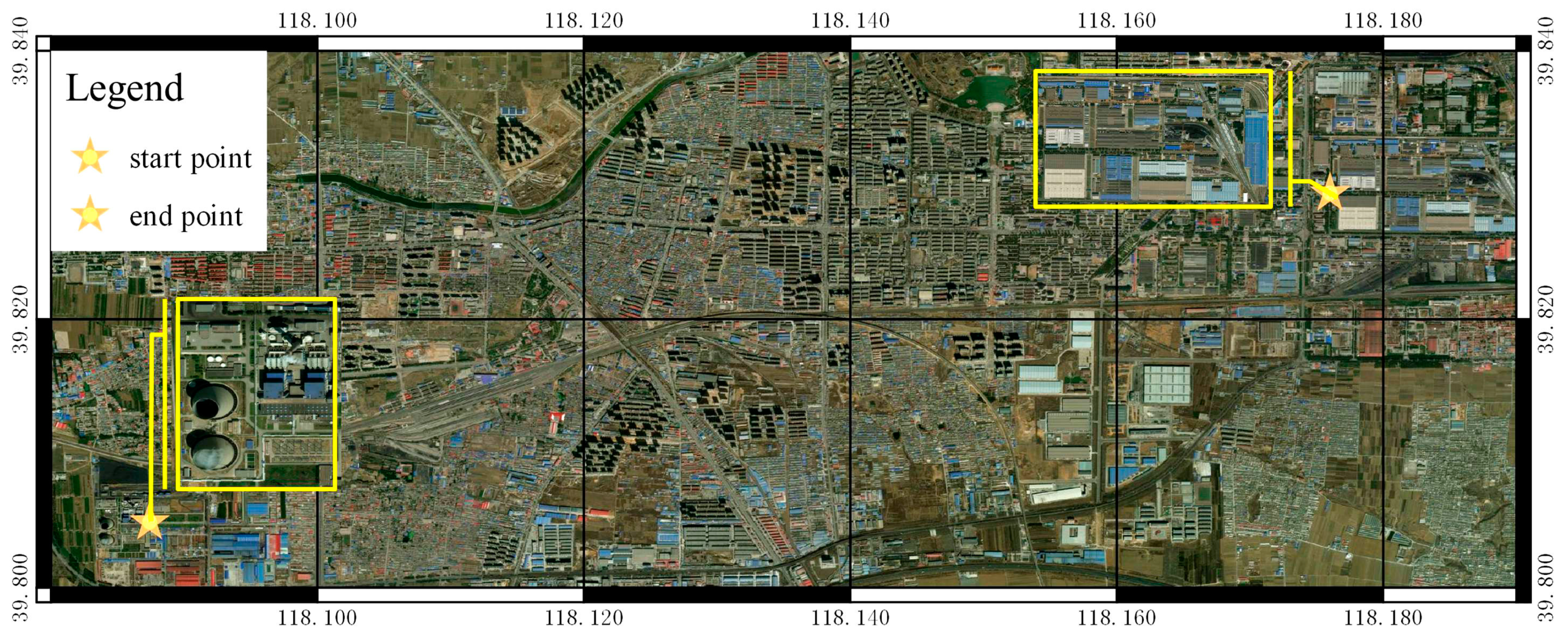
2.1. Study Area

The DH project lies in Tangshan City, Hebei Province. The project starts from the Fengrun cogeneration plant and ends at the China railway rolling stock corporation. It aims mainly for industrial heating as well as residential heating along the route. The project was constructed in 2017–2018. After the implementation of the project, the emissions of greenhouse gases and pollutants can be reduced significantly. Figure 1 shows the remote sensing image of the study area acquired from Google Earth. Google Earth’s imageries are retrieved from satellites or aircraft. The spatial resolutions are from 15 meters to 15 centimeters. In this paper, we cut the latest image of the study area. From Figure 1, we can generally find that the land-cover types are mainly road, vegetation, water, buildings, and bare land.

2.2. DH Route Planning Indicator (DHRPI) Definition

It is of great importance for stakeholders to evaluate the alternative DH routes by indicators. The ACS algorithm can select the best route by solving the cost function. Therefore, we chose the remote sensing image as the data source, and designed the cost function as the sum of the weighted classified pixels that the route covered. Then, the DHRPI is defined as the cost function values. The route with the minimum DHRPI is treated as the optimum route.

According to the design code for the city heating network (CJJ 34-2010) [38], heating pipes through non-built areasshould belaid along the highway in priority. To get the weights of different land-cover types, we invited a panel of experts from Beijing Gas and Heating Engineering Design Institute and North China Power Engineering Co., Ltd., and forecasted the weights by the Delphi method [39,40]. The weights of the road, bare land, vegetation, building groups, and water were set to 0.0477, 0.0953, 0.190, 0.286, and 0.381, respectively.

Roads are broken into numerous segments at the intersections. The endpoints and the intersections constitute the elementary entities (nodes). Suppose that nodes i and j belong to the same road. Then, the cost c_i,j (or c_j,i) is the sum of the weights of the pixels that the real road segment covered, as shown in Equation (1):

$$c_{i,j}=wr\times {\displaystyle \sum _{p=1}^{r}I{R}_p}$$

(1)

where p is the pixel number of the road segment covered. IR is the binary image of road. IR_p refers to the exact road pixel, and the value is set to one. wr represents the weights of the road.

Otherwise, if i and j belong to different roads, then the cost c_i,j (or c_j,i) is the sum of the weights of the pixels that the linear segment from i to j (or j to i)covered, as shown in Equation (2):

$$c_{i,j}={\displaystyle \sum _{p=1}^s(IB{L}_p\times wbl+I{V}_p\times wv+I{W}_p\times ww+I{B}_p\times wb)}$$

(2)

where p is the pixel number of the linear segment covered. IBL, IV, IB, and IW are the binary images of bare land, vegetation, building, and water. wbl, wv, wb, and ww represent the weights of bare land, vegetation, building, and water, respectively. One can trace the corresponding row and column numbers of p in the binary images. For instance, if the location of p is a bare land pixel, then the IBL_p is 1, and IV_p, IW_p, and IB_p are 0, so only the wbl has an effect on the c_ij.

Through computing the cost of every two nodes, we can derive a cost matrix C_n×n, as shown in Equation (3):

$$C=\left(\begin{array}{cccc}{c}_{1,1}& c_{1,2}& \dots & c_{1,n}\\ c_{2,1}& c_{2,2}& \dots & c_{2,n}\\ \dots & \dots & \dots & \dots \\ c_{n,1}& c_{n,2}& \dots & c_{n,n}\end{array}\right)(i,j\in [1,n])$$

(3)

where c_ij means the cost of the edge connecting node i and j.

Then, the DHRPI can be derived by Equation (4):

$$f_{ind}={\displaystyle \sum _{n=1}^{N-1}{D}_{\mathrm{n},\mathrm{n}+1}}$$

(4)

where n is the sequential number of the nodes of the route passed. N is the total node number of the route covered. D_n,n+1 is the cost of the specific segment, and it can be traced to c_i,j by the index of the node.

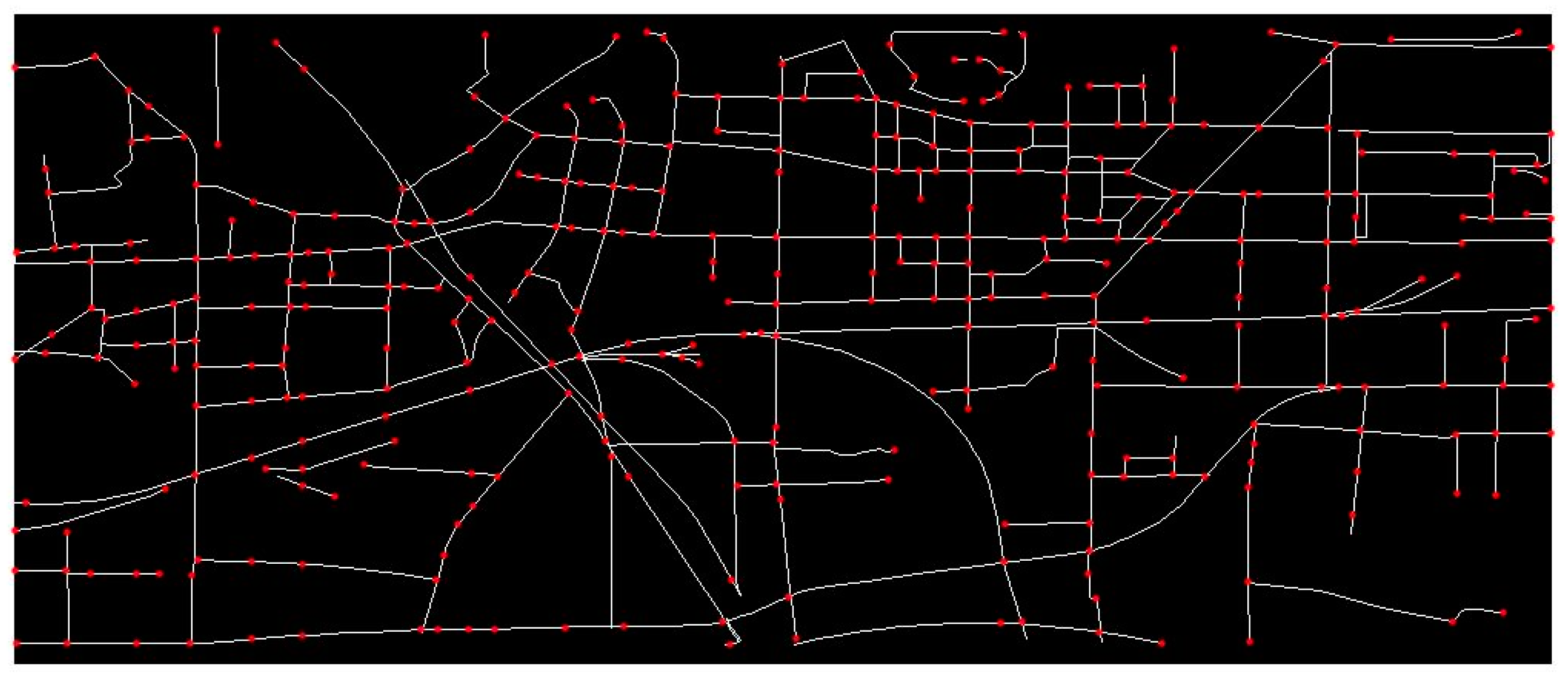
2.3. Data Preparation

In this paper, Google Earth imagery is treated as the primary data source. The node distribution data store the node locations (i.e., row and column numbers) in the Google Earth imagery. The classification data can be extracted from the image and stored as the binary image. Different land covers are given different weights. Both the node distribution data and the classification data are substituted into Equation (2) for the DHRPI calculation as described in Section 2.2. Besides the Google Earth imagery, we select OpenStreetMap (OSM) as an auxiliary data source. OSM is a prominent example of volunteered geographic information. OSM data can be downloaded from the official website (https://www.openstreetmap.org/) given the exact coordinate range. The downloaded OSM file contains point, line, and polygon features. We pay more attention to the lines and polygons, which represent most roads and buildings. However, volunteered geographic informationinevitably has some data redundancy and data loss. Therefore, we further supplemented and revised the classifications with the help of an open source QGIS platform based on the remote sensing imagery from Google Earth. Road, bare land, vegetation, building groups, and water were extracted in detail. Figure 2a is the downloaded data from OSM, while Figure 2b is the classification map reprocessed by QGIS and the remote sensing imagery. The processed file was converted to the “.shp” format.

Based on the lines of roads, we extracted the nodes. As shown in Figure 3, there are in total 361 nodes in the study area.

With the help of ENVI software (a geospatial imagery analysis and processing application) [41,42], we derived the binary images as shown in Figure 4. Combining the weights we assigned for different classifications, we can calculate the cost between every two nodes. Thus, a 361 × 361 cost matrix was obtained.

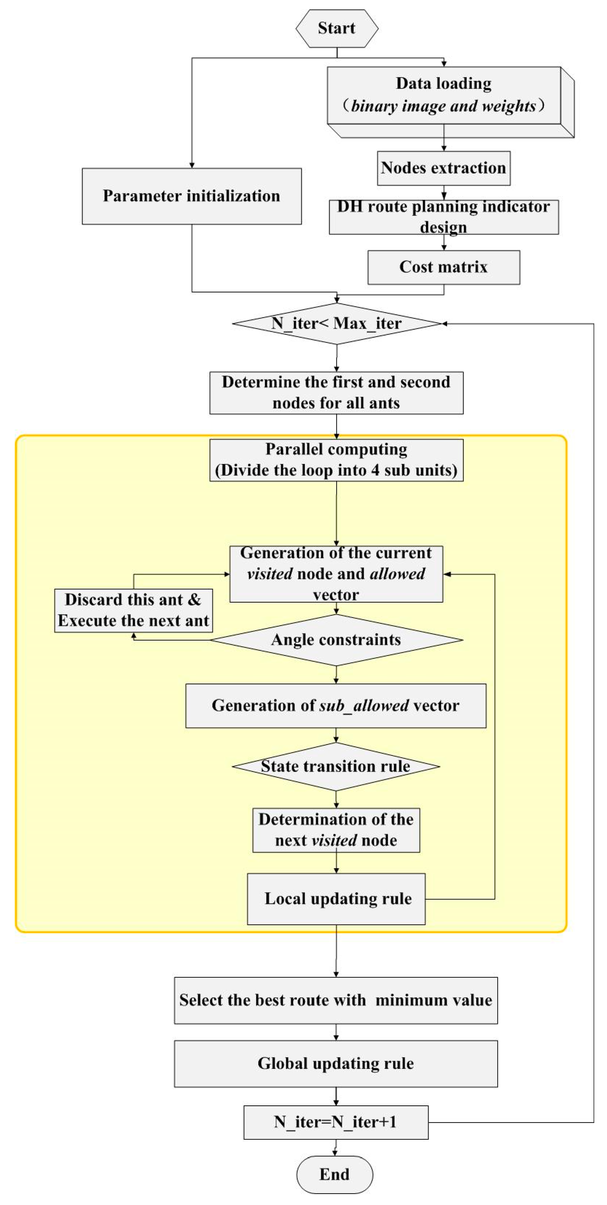
2.4. Parallel ACS Algorithm

In this paper, we chose ACS as our algorithm prototype and modified the ACS algorithm to suit the DH route design problem. Moreover, to improve the efficiency, we convert ACS to a parallel version. The principle of the algorithm is described as follows:

2.4.1. Parameter Initialization

As mentioned in Section 2.2 and Section 2.3, the number of nodes (n) is 361, and a 361 × 361 cost matrix (C) has been prepared. The pheromone matrix is set the same dimension as the cost matrix, which stores the pheromone between every two nodes. The initial value of the pheromone (${\tau }_0$) is set at 1.0 for all the edges. The number of ants (m) is set to 36, considering both the diversity and the efficiency. Among the 361 nodes, the start point of the route (Sp) is fixed on the 238th node, while the end point of the route (Ep) is the 216th node. We also determine the heuristic information (${\eta }_{ij}$) as the inverse of the edge’s cost, which can be expressed as Equation (5):

$${\eta }_{ij}=1/c_{ij}$$

(5)

The index of visited nodes are stored in a m×n matrix named Tabu. As to the current ant, the index of the visited nodes are stored in a vector named visited, while the index of the candidate nodes are stored in a vector named allowed. $allowed\cup visited$ comprises the total 361 nodes.

2.4.2. Route Searching

As the Sp and the Ep are fixed, the search starts from the second point and ends when meeting the Ep. The effective route is limited from Sp to Ep. There are several points that need attention in the route searching process:

• The parallelization of the route searching

The route searching algorithm is converted to a parallel one to further improve the efficiency. In this paper, the number of nodes is 361, and the number of ants is 36. The time spent on the route searching procedure takes the largest proportion. Since we develop the code with MATLAB software on a computer with a quad core CPU systems (Intel(R) Core(TM) i5-6500 CPU @3.2GHz), the route searching algorithm is divided into four parallel algorithms. Therefore, every thread has nine ants executing the searching. The angle constraint module, the state transition rule module, and the local updating rule module mentioned below are executed separately for different threads. Theoretically, the operating efficiency can be around four times compared to the sequential algorithm.

• The angle constraint module

The angle constraint is introduced to further screen the alternative nodes. In ACS, ant selects the next node to reach from the allowed vector. However, according to the Design Code For the City Heating Network (CJJ 34-2010) [39], the DH route should have no intersections, and the crossing angle should be more than 90°. Therefore, it is a prerequisiteto screen the nodes satisfying the angle requirement from the allowed vector. An angle judgment model based on the cosine law is introduced as shown in Equation (6):

$$\begin{array}{l}fori=1:N_{allowed}\\ \hspace{1em}a=\sqrt{{(X_{this}-X_{last})}^2+{(Y_{this}-Y_{last})}^2}\\ \hspace{1em}b=\sqrt{{(X_{this}-X_{next})}^2+{(Y_{this}-Y_{next})}^2}\\ \hspace{1em}c=\sqrt{{(X_{next}-X_{last})}^2+{(Y_{next}-Y_{last})}^2}\\ \hspace{1em}\cos \theta =\frac{(a^2+b^2-c^2)}{2ab}\\ \hspace{1em}if\cos \theta <0\\ \hspace{1em}\hspace{1em}discard{P}_{next}(X_{next},Y_{next})\\ \hspace{1em}end\\ end\end{array}$$

(6)

where N_allowed is the size of the allowed vector. $P_{next}(X_{next},Y_{next})$ is one of the points from the allowed vector, while $P_{this}(X_{this},Y_{this})$ and $P_{last}(X_{last},Y_{last})$ are the current point and the previous point. After the angle screening step, a subset of the allowed vector, namely sub_allowed, is acquired, and used for the subsequent calculations.

Due to the stricter angle constraints, it is possible that the search is finished without meeting the Ep. In this case, the ant and the route are given up, and they no longer participates in the updating and cost function calculation.

• The state transition rule module

The ant selects the next node according to the ACS state transition rule. A random number q is generated and used for the next node selection. The rule is given by Equation (7):

$$\{\begin{array}{l}\arg \max \left\{{[{\tau }_{ij}(t)]}^{\alpha }{[{\eta }_{ij}(t)]}^{\beta }\right\},\hspace{1em}\hspace{1em}\hspace{1em}\hspace{1em}\hspace{1em}\hspace{1em}\hspace{1em}\hspace{1em}\left(7\text{-}1\right)\hspace{1em}\hspace{1em}\hspace{1em}q\le q_0\\ \hspace{1em}{p}_{ij}^k(t)=\{\begin{array}{ccc}\frac{{[{\tau }_{ij}(t)]}^{\alpha }\times {[{\eta }_{ij}(t)]}^{\beta }}{{\displaystyle \sum _{k\in sub\_allowe{d}_k}{[{\tau }_{ik}(t)]}^{\alpha }\times {[{\eta }_{ik}(t)]}^{\beta }}},& j\in allowe{d}_k& \left(7\text{-}2\right)\\ 0& & (7\text{-}3)\end{array}\hspace{1em}\hspace{1em}q>q_0\end{array}$$

(7)

where q is a random number uniformly distributed in [0,1], and q_o is a constant. Here, we set q₀ = 0.9 as a reference [16]. i is the current node, while j is any one candidate node from the sub_allowed vector. ${\tau }_{ij}(t)$ is the intensity of the pheromone between i and j at time t. ${\eta }_{ij}(t)$ is the heuristic information between i and j at time t. sub_allowed_k stores the candidate nodes. α and β are two constantsthat can be described as the weighted values of the pheromone (${\tau }_{ij}(t)$) and heuristic information (${\eta }_{ij}$), respectively. Here, we set α = 0.1 and β = 2 as references [16].

Since the ant favors choosing the next node with a short edge and a large amount of pheromone, when q ≤ q₀, we directly set the next visited node to the one with the maximum value, as shown in (7-1). Otherwise, when q > q₀, the roulette wheels method is executed. For every j belongs to sub_allowed_k, $p_{ij}^k(t)$ is calculated by Equation (7-2), given a random generated number p, and the node with $p_{ij}^k(t)$≥ p is chosen as the next visited node. If j doesn’t belong to sub_allowed_k, $p_{ij}^k(t)$ is set to 0 as shown in Equation (7-3). We can determine that the search is finished for one ant when Ep is chosen as the next visited node.

• The local updating rule module

A local updating rule is applied once the next node is fixed as reference [16]. The local updating rule is described as shown in Equation (8):

$${\tau }_{ij}=(1-\rho ){\tau }_{ij}+\rho ·△{\tau }_{ij}^{}$$

(8)

where i is the current node, and j is the next node that the ant has chosen. 0 < ρ < 1, and ρ is a parameter; here, we set ρ = 0.1. $△{\tau }_{ij}^{}$ is set the same as the initial value of pheromone (${\tau }_0$), i.e., $△{\tau }_{ij}^{}$= 1.0.

The first part of Equation (8) represents the evaporation of the pheromone, while the second part represents the reinforcement of the pheromone. With the help of the local updating rule, the route is shuffled dynamically, and the search can take full advantage of the pheromone information. It is worth noting that the pheromone updating is only focused on the current iteration and the segments between the start point and the end point.

2.4.3. Pheromone Updating

After all the ants complete their trip for one iteration, the path’s pheromone intensity should be updated. Here, we conduct the global updating rule as ACS. Only the globally best ant is allowed to deposit pheromones. The formulation is shown in Equation (9):

$${\tau }_{ij}=(1-\alpha ){\tau }_{ij}+\alpha ·△{\tau }_{ij}^{}$$

(9)

where i and j are the nodes belonging to the best route, 0 < α < 1, and α is the pheromone decay parameter; here, we set α = 0.1. The first part of Equation (9) represents the evaporation of the pheromone, while the second part represents the reinforcement of the pheromone. $△{\tau }_{ij}^{}$ is defined as shown in Equation (10):

$$△{\tau }_{ij}^{}=\{\begin{array}{cc}{(L_{best})}^{-1},\hfill & \hfill if(i,j)\in global\_best\_route\\ 0,\hfill & \hfill otherwise\end{array}$$

(10)

where $L_{best}$ is the DHRPI of the best route. It is worth noting that the pheromone updating is only focused on the segments between the start point and the end point.

Based on the description of the aforementioned algorithm principle, we can get the flowchart of the parallel ACS for DH route design, as shown in Figure 5. It should be noted that the yellow part is the route searching module, and executes parallel computing.

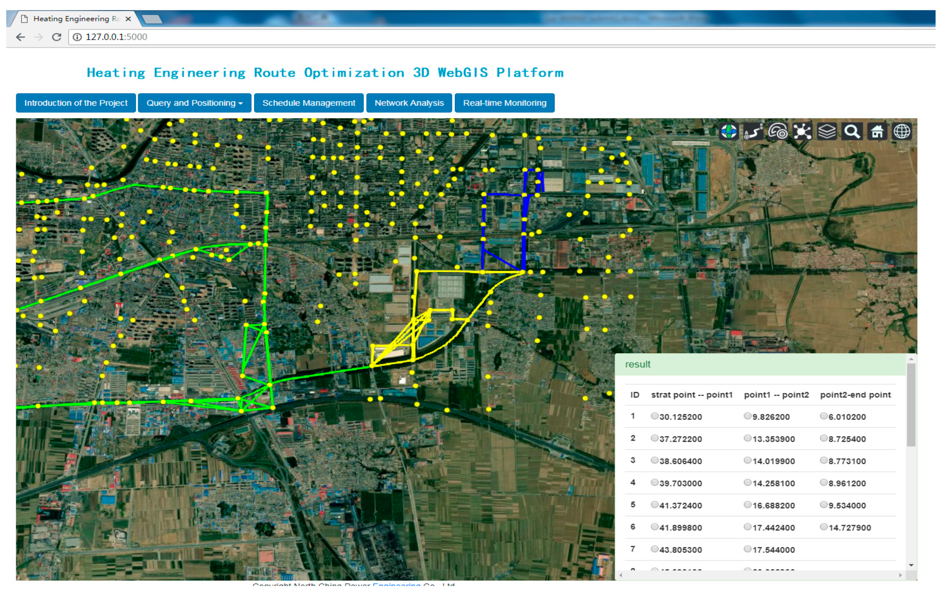
2.5. Interactive 3D WebGISTool

We present a 3D WebGIS platform for the route designers. The platform combines the parallel ACS algorithm as well as the 3D visualization function. HTML and CSS are used to design the front end. The parallel ACS algorithm is developed by MATLAB and is invoked by the platform using python. The Cesium visualization engine is introduced toachieve the 3D visualization. As a case study, we put the website on the server of our corporation.

With this platform, the interactive design can be realized. Users can assign no more than five favorite points that the route must pass. The selected nodes are treated as the new starting point and end point, and the study area is divided into several sub zones. The identification (ID) numbers of the user-defined points are transferred to the back-end and invoked by the algorithm. As shown in Figure 6, the starting point and the end point are expressed in orange, and points 1 and 2 (red points) are the user-defined mandatory passed nodes.

The best routes for all subsets are calculated accordingly. The final best route can be derived by linking the best sub routes end to end. Users can define the number of the best routes to be presented. As shown in Figure 7, the candidate routes and the indicators are displayed on thelower right corner of the user interface. The alternative routes of the first, second, and third sub zone are displayed in green, yellow, and blue, respectively. Then, users can compare all of them and pick the most appropriate one.

3. Results and Discussion

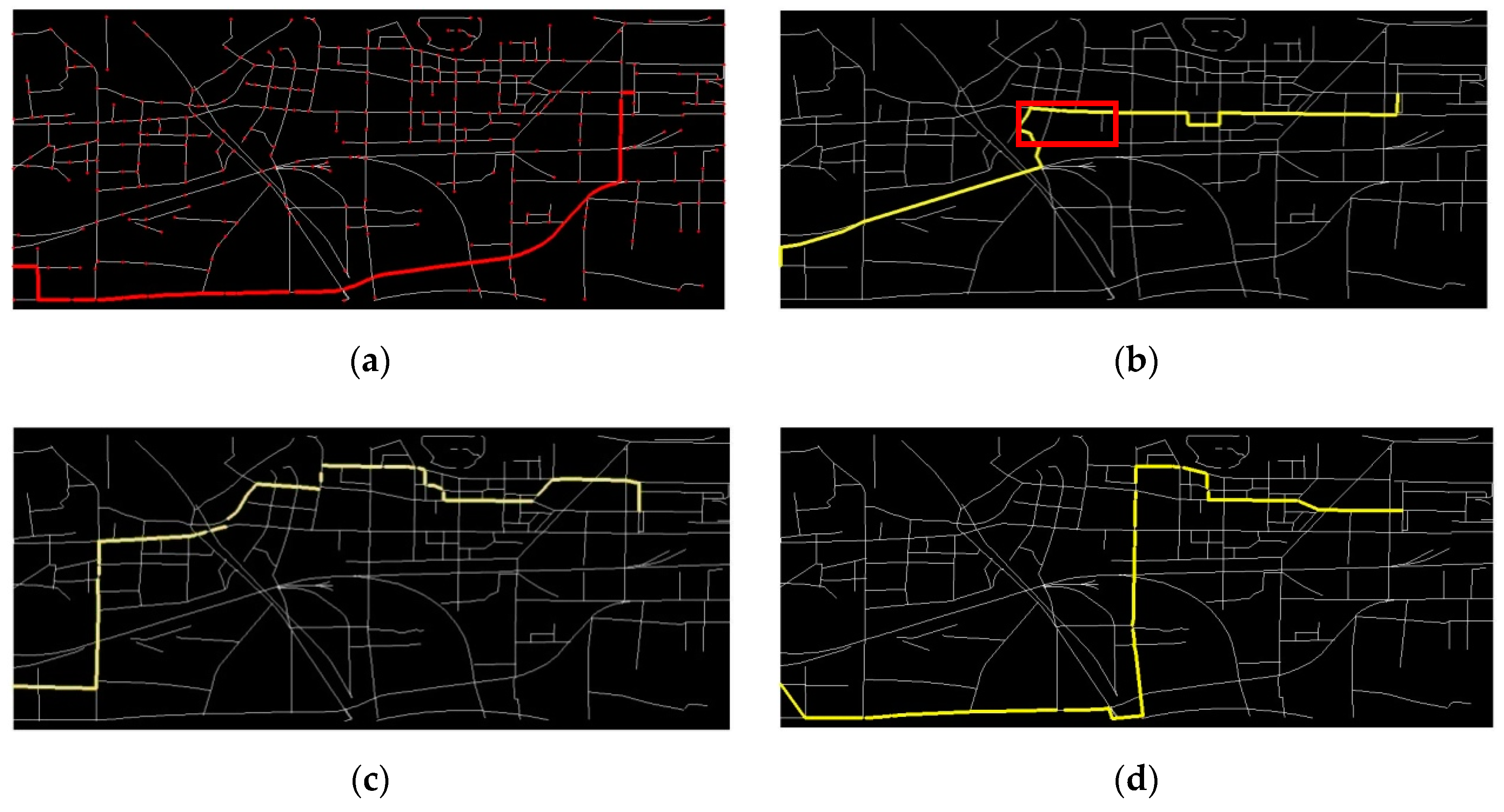
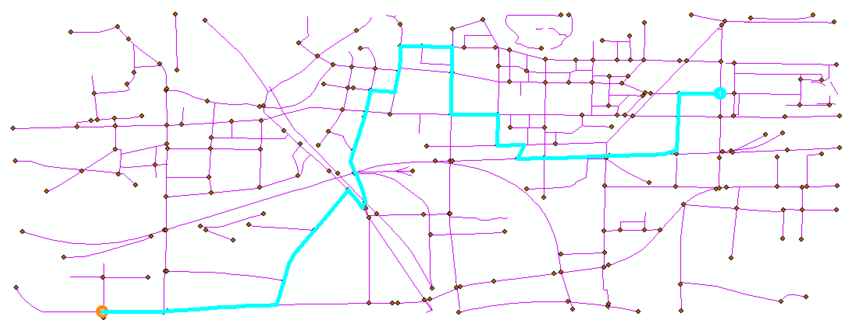
3.1. Comparation with the Manually Designed Route

We set the number of iterations as 100 and repeated them 10 times to verify the stability. The indicators of the top 30 best routes areshown in

Table 1. The indicators of the top 30 best routes.

No.	Indicators	No.	Indicators	No.	Indicators
1	29.2184	11	36.5449	21	38.8374
2	30.2141	12	36.7126	22	39.1459
3	30.7896	13	36.9894	23	39.8428
4	31.9826	14	37.1286	24	39.905
5	32.0779	15	37.2763	25	41.9456
6	32.3144	16	37.4986	26	42.3429
7	32.6468	17	37.9436	27	44.4666
8	33.5068	18	38.231	28	45.2416
9	36.2242	19	38.5003	29	47.052
10	36.3235	20	38.6646	30	48.335

. We can illustrate that the value of the manually selected route (46.22) is between the 28th (45.24) and the 29th (47.05) best performers.

Figure 8 shows the manually designed route (a), as well as the first (b), the 28th (c), and the 29th (d) routes selected by our algorithm. Compared to the manually selected route, the parallel ACS can derive the routes with even smaller indicators. However, the best route isnear a railway station (red rectangular area), as shown in Figure 8b. It is not a good choice to lay the DH pipe near a railway, because the underground engineering may cause hidden trouble with safety. Considering all the situations, the algorithm can give more alternatives for decision making. It can greatly reduce the repeated reconnaissance and save a lot of time.

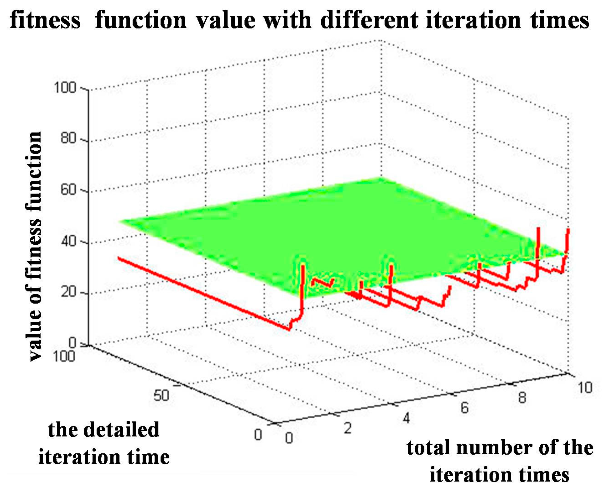
3.2. Comparation with the Corresponding Sequential Algorithm

The average operating time of our parallelACS algorithm is 3.912 seconds for one iteration (36 ants divided into four groups, every group contains nine ants), while the corresponding sequential algorithm costs 18.736 seconds for one iteration (containing 36 ants). Considering that there are four cores of our computer, the efficiency is increased 4.789 times. Additionally, we analyzed the convergence of the algorithm. As shown in Figure 9, the green plane is the DHRPI of the manually selected route, while the red lines are the indicators of 10 repetitions from the first iteration to the 100th iteration, respectively. We can illustrate that all 10 repetitions can reach the minimum DHRPI within 30 iterations.

3.3. Comparation with ArcGIS Network Analyst Tool

As for the ArcGIS platform, we used ArcGIS 10 to fulfill the job. The ArcGIS 10 Network Analyst tool can find the shortest route based on the well-known Dijkstra algorithm. The shape file of the road was loaded into the layer, and a network dataset was built with the wizard. The edges and junctions of the network were generated at the end of the wizard. Since the original vertex may be inadequate, we have to split the roads at the junctions manually. Then, the network analyst can be executed by setting two stops. Figure 10 shows the best route solved by ArcGIS. Although the Dijkstra’s algorithm can solve the DH routing problem given the weighted cost of different edges, the integrated ArcGIS network analyst tool is not quite specific to the DH routing design problem compared to our platform. For example, the route selection is considered only along the roads. However, in reality, the route selection may be laid across the vegetation, rivers, or other land covers comprehensively considering length and cost. Additionally, in ArcGIS, users can get the best route with less quantitative information. It is not flexible enough for designers to compare several candidate routes.

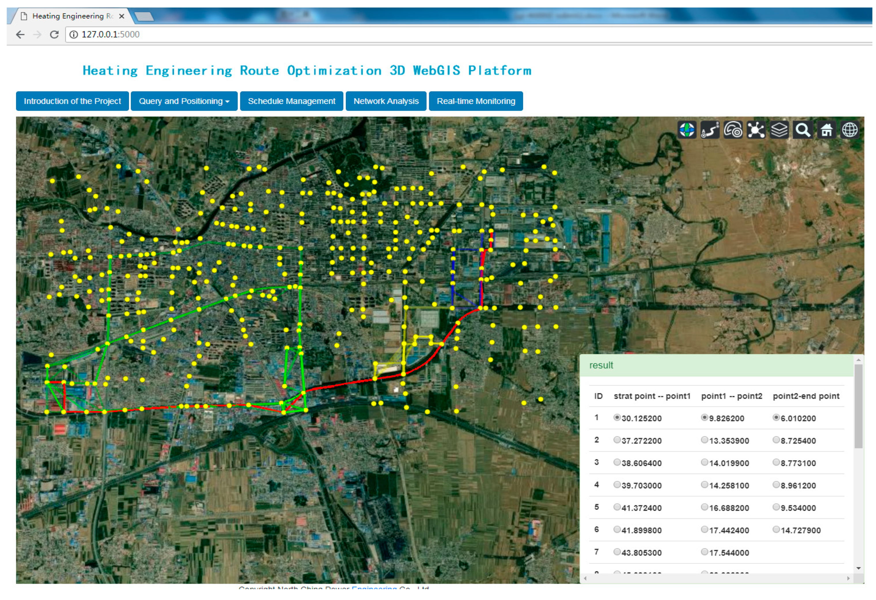
3.4. Interactive Design Results of the 3D WebGIS Tool

As shown in Figure 6 and Figure 7, by defining the mandatory passed points, users can design the route interactively. Figure 11 shows the best operation result (the red line). By appointing two intermediate points, the platform can get the best route, which is even the same as the manually selected one.

4. Conclusions

This paper provides a DHRPI to estimate the quality of the alternative heating routes. Remote sensing imagery and the OpenStreetMap data act as the data sources. A parallel ACS algorithm suitable for the DH route design is proposed, which performs as the first contribution of this paper. The second contribution is the development of a convenient tool for the DH route preliminary design. The tool combines the proposed parallel ACS algorithm and the 3D WebGIS technology. It is applied to the route design of the Fengrun heating engineering project. Compared to the manually-selected route, as well as the commercial ArcGIS platform, the study illustrates that our algorithm can get 28 candidate routes with smaller indicators than the manually selected DHRPI (46.22). The average operating time of our parallel ACS algorithm is 3.912 seconds for one iteration (36 ants divided into four groups, every group contains nine ants), which condensed by 4.789 times for the corresponding sequential algorithm. The algorithm can reach the minimum DHRPI within 30 iterations. Additionally, the proposed 3D WebGIS tool with our improved ACS algorithm is more flexible and user-friendly, and is aimed at the heating route design. The platform has the following features:

(1). The platform integrates our parallel ACS algorithm, which can provide the best heating route automatically and efficiently.

The remote sensing-based heating route planning indicator, the weighted cost matrix, and the updating strategy of the ACS algorithm are proposed to suit the specific heating route requirements. Additionally, the parallel pattern is proposed to shorten the operating time. With the help of the parallel ACS algorithm, we can give a quantitative assessment for the alternative routes.

(2). The platform combines the 3D WebGIS technology in which users can design the DH route intuitively and interactively.

The open source Cesium engine is introduced to realize the rendering and visualization of 3D scenes. The WebGIS technology is adopted to provide the light weighted platform. As the algorithm and the platform are based on an open source 3D engine and independent development, the platform can be continuously maintained and improved.

Still, there is much that can be done to improve the performance of our platform. For example, in this study, we generally set different weights of different land-cover types to represent different factors (e.g. excavation cost, compensation for demolition and resettlement, pipe materials, the impact on traffic, and so on). The weights are roughly calculated by the Delphi method. A more accurate cost estimation is required. Additionally, the 3D visualization has not reached its full potential. Since the main DH project is under ground, the excavation depth should be taken into account for the cost calculation. Considering the movement of water and the elimination of air, the pipe should have a certain slop. Moreover, there are complex pipe networks for other uses at different depth and different directions; thus, the design of the DH route should pay attention to avoid collision. All of them require the introduction of the elevation information. However, most of the information is undisclosed. Therefore, in this paper, we focused on the preliminary design of the DH route and the realization of the 3D platform. Our future work will aim at improving the algorithm and platform built in this paper for further detailed design, especially the 3D design.

References

1. Li, H.; Svendsen, S. District heating network design and configuration optimization with genetic algorithm. J. Sustain. Dev. Energy Water Environ. Syst. 2013, 1, 291–303. [Google Scholar] [CrossRef]
2. Bloomquist, R.G. Geothermal district energy system analysis, design, and development. Available online: https://pangea.stanford.edu/ERE/pdf/IGAstandard/ISS/2001Romania/bloomquist_dh.pdf (accessed on 15 April 2019).
3. Yildirim, N.; Toksoy, M.; Gokcen, G. Piping network design of geothermal district heating systems: Case study fora university campus. Energy 2010, 35, 3256–3262. [Google Scholar] [CrossRef]
4. Dobersek, D.; Goricanec, D. Optimization of tree path pipe network with nonlinear optimization method. Appl. Therm. Eng. 2009, 29, 1584–1591. [Google Scholar] [CrossRef]
5. Li, X.; Duanmu, L.; Shu, H. Optimal design of district heating and cooling pipe network of seawater-source heat pump. Energy Build. 2010, 42, 100–104. [Google Scholar] [CrossRef]
6. Valdimarsson, P. PipeLab 3.18 Software. NuonTechnischBedrijf; University ofIceland: Reykjavík, Iceland, 2002. [Google Scholar]
7. Dorigo, M.; Maniezzo, V.; Colomi, A. The Ant System: An Autocatalytic Optimizing Process. Available online: http://citeseerx.ist.psu.edu/viewdoc/citations;jsessionid=C806753D4246E244F6BF5A5B82397014?doi=10.1.1.51.4214 (accessed on 15 April 2019).
8. Karaboga, D. An Idea Based on Honey Bee Swarm for Numerical Optimization. Available online: http://citeseerx.ist.psu.edu/viewdoc/summary?doi=10.1.1.714.4934 (accessed on 15 April 2019).
9. Yang, X.-S.; Deb, S. Cuckoo Search Via Lévy Flights. In Proceedings of the World Congress on Nature & Biologically Inspired Computing (NaBIC), Coimbatore, India, 9–11 December 2009; pp. 210–214. [Google Scholar]
10. Shah-Hosseini, H. The intelligent water drops algorithm: A nature-inspired swarm-based optimization algorithm. Int. J. Bio-Inspired Comput. 2009, 1, 71–79. [Google Scholar] [CrossRef]
11. Lawler, E.L.; Lenstra, J.K.; Kan, A.R.; Shmoys, D.B. The Traveling Salesman Problem: AguidedTour of Combinatorial Optimization; Wiley: Chichester, UK, 1985. [Google Scholar]
12. Zhang, Y.; Zhao, H.; Cao, Y.; Liu, Q.; Shen, Z.; Wang, J.; Hu, M. A hybrid ant colony and cuckoo search algorithm for route optimization of Heating engineering. Energies 2018, 11, 2675. [Google Scholar] [CrossRef]
13. Dorigo, M.; Maniezzo, V.; Colorni, A. Ant system: Optimization by a colony of cooperating agents. IEEE Trans. Syst. Man. Cybern. Part B 1996, 26, 29–41. [Google Scholar] [CrossRef] [PubMed]
14. Bullnheimer, B.; Hartl, R.F.; Strauss, C. A new rank-based version of the ant system: A computational study. Cent. Eur. J. Oper. Res. Econ. 1999, 7, 25–38. [Google Scholar]
15. Stützle, T.; Hoos, H. MAX–MIN Ant System and Local Search for the Traveling Salesman Problem. In Proceedings of the 1997 IEEE International Conference on Evolutionary Computation (ICEC’97), Indianapolis, IN, USA, 13–16 April 1997; pp. 309–314. [Google Scholar]
16. Dorigo, M.; Gambardella, L.M. Ant colony system: A cooperative learning approach to the traveling salesman problem. IEEE Trans. Evol. Comput. 1997, 1, 53–66. [Google Scholar] [CrossRef]
17. Yu, B.; Yang, Z.-Z.; Yao, B. An improved ant colony optimization for vehicle routing problem. Eur. J. Oper. Res. 2009, 196, 171–176. [Google Scholar] [CrossRef]
18. Tuba, M.; Jovanovic, R. Improved ACO algorithm with pheromone correction strategy for the traveling salesman problem. Int. J. Comput. Commun. 2013, 8, 477–485. [Google Scholar] [CrossRef]
19. Dorigo, M.; Stützle, T. Ant Colony Optimization: Overview and Recent Advances. In Handbook of Metaheuristics; Gendreau, M., Potvin, J.Y., Eds.; Springer: New York, NY, USA, 2009. [Google Scholar]
20. Gambardella, L.M.; Taillard, E.D.; Agazzi, G. MACS-VRPTW: A Multiple Ant ColonySystem for Vehicle Routing Problems with Time Windows. In New Ideas in Optimization; Corne, D., Dorigo, M., Glover, F., Eds.; McGraw Hill: London, UK, 1999; pp. 63–76. [Google Scholar]
21. Mahi, M.; Baykan, Ö.K.; Kodaz, H. A new hybrid method based on particle swarm optimization, ant colony optimization and 3-opt algorithms for traveling salesman problem. Appl. Soft Comput. 2015, 30, 484–490. [Google Scholar] [CrossRef]
22. Tsutsui, S.; Fujimoto, N. Parallel Ant colony optimization algorithm on a multi-core processor. In Proceedings of the 7th International Conference onSwarm Intelligence, Brussels, Belgium, 8–10 September 2010; pp. 488–495. [Google Scholar]
23. Delévacq, A.; Delisle, P.; Gravel, M.; Krajecki, M. Parallel ant colony optimization on graphics processing units. J. Parallel Distrib. Comput. 2013, 73, 52–61. [Google Scholar] [CrossRef]
24. Pedemonte, M.; Nesmachnow, S.; Cancela, H. A survey on parallel ant colony optimization. Appl. Soft Comput. 2011, 11, 5181–5197. [Google Scholar] [CrossRef]
25. Arcgis Online. Available online: www.arcgis.com (accessed on 15 April 2019).
26. Kallel, A.; Serbaji, M.M.; Zairi, M. Using GIS-based tools for the optimization of solid waste collection and transport: Case study of Sfax City, Tunisia. J. Eng. 2016, 10, 1–7. [Google Scholar] [CrossRef]
27. Abousaeidi, M.; Fauzi, R.; Muhamad, R. Geographic Information System (GIS) modeling approach to determine the fastest delivery routes. Saudi J. Biol. Sci. 2016, 23, 555–564. [Google Scholar] [CrossRef] [PubMed]
28. Alazab, A.; Venkatraman, S.; Abawajy, J.; Alazab, M. An Optimal Transportation Routing Approach Using GIS-Based Dynamic Traffic Flows. In Proceedings of the International Conference on Management Technology and Applications, Singapore, 10–12 September 2010; pp. 172–178. [Google Scholar]
29. Baufumé, S.; Grüger, F.; Grube, T.; Krieg, D.; Linssen, J.; Weber, M.; Stolten, D. GIS-based scenario calculations for a nationwide German hydrogen pipeline infrastructure. Int. J. Hydrog. Energy. 2013, 38, 3813–3829. [Google Scholar] [CrossRef]
30. Google Earth. Available online: http://earth.google.com (accessed on 15 April 2019).
31. Skyline. Available online: http://www.skylineglobe.cn/ (accessed on 15 April 2019).
32. Website of Super map. Available online: http://www.supermap.com/cn/ (accessed on 15 April 2019).
33. Website of EV-Globe. Available online: http://www.ev-image.com/products/l-3852968750166. html (accessed on 15 April 2019).
34. NASA WorldWind Project Suspension Update. Available online: https://worldwind.arc.nasa.gov/ (accessed on 15 April 2019).
35. Website of Cesium. Available online: http://cesiumjs.org/ (accessed on 15 April 2019).
36. Torres-Martínez, J.A.; Seddaiu, M.; Rodríguez-Gonzálvez, P.; Hernández-López, D.; González-Aguilera, D. A Multi-Data Source and Multi-Sensor Approach for the 3D Reconstruction and Visualization of a Complex Archaelogical Site: The Case Study of Tolmo De Minateda. Int. Arch. Photogramm.Remote Sens. 2015, XL-5/W4, 37–44. [Google Scholar]
37. Gobakis, K.; Mavrigiannaki, A.; Kalaitzakis, K.; Kolokotsa, D.-D. Design and Development of a Web Based GIS Platform for Zero energy Settlements Monitoring. In Proceedings of the 9th International Conference on Sustainability in Energy and Buildings, Chania, Greece, 5–7 July 2017; pp. 48–60. [Google Scholar]
38. People’s Republic of China Ministry of Housing and Urban-Rural Development. Design Code for City Heating Network; CJJ 34-2010; China Building Industry Press: Beijing, China, 2011.
39. Dalkey, N.; Helmer, O. An experimental application of the Delphi method to the use of experts. Manag. Sci. 1963, 9, 458–467. [Google Scholar] [CrossRef]
40. Rowe, G.; Wright, G. The Delphi technique as a forecasting tool: Issues and analysis. Int. J. Forecast. 1999, 15, 353–375. [Google Scholar] [CrossRef]
41. Website of ENVI/IDL. Available online: http://www.enviidl.com/ (accessed on 15 April 2019).
42. Website of ENVI. Available online: https://www.harrisgeospatial.com/ (accessed on 15 April 2019).
Figure 1. The location of the heating engineering project.
Ijgi 08 00225 g001
Figure 2. Classification data of the study area. (a) The downloaded data from OSM; (b) The reprocessed classification maps.
Ijgi 08 00225 g002
Figure 3. The distribution of roads and nodes.
Ijgi 08 00225 g003
Figure 4. Classification maps of the study area. (a) Binary image of roads; (b) Binary image of buildings; (c) Binary image of water; (d) Binary image of vegetation; (e) Binary image of bare land; (f) Distribution of nodes.
Ijgi 08 00225 g004
Figure 5. Flowchart of the parallel ant colony system (ACS) algorithm.
Ijgi 08 00225 g005
Figure 6. The interactive design interface by assigning the mandatory passed nodes (red points).
Ijgi 08 00225 g006
Figure 7. Scheme comparison interface with alternative routes of the three sub zones (green ones for the first zone, yellow ones for the second zone, and blue ones for the third zone).
Ijgi 08 00225 g007
Figure 8. District heating (DH) routes by manual design and the algorithm (cost function value sorted from the smallest to the biggest). (a) The manually designed route; (b) The route with minimum cost function value; (c) The 28th route; (d) The 29th route.
Ijgi 08 00225 g008
Figure 9. The cost function value variation from thefirst iteration to the 100th iteration for the 10 repetitions.
Ijgi 08 00225 g009
Figure 10. The best route solved by ArcGIS.
Ijgi 08 00225 g010
Figure 11. Best route solved by the interactive design platform (red line).
Ijgi 08 00225 g011