Anisotropic Diffusion for Improved Crime Prediction in Urban China

1
State Key Lab of Information Engineering in Surveying Mapping and Remote Sensing, Wuhan University, Wuhan 430079, China
2
Collaborative Innovation Center of Geospatial Technology, Wuhan 430079, China
3
Key Laboratory of Aerospace Information Security and Trusted Computing of the Ministry of Education, Wuhan University, Wuhan 430079, China
4
Key Laboratory of Police Geographic Information Technology, Ministry of Public Security, Changzhou 213022, China
5
Urban Informatics & Spatial Computing Lab, New Jersey Institute of Technology, Newark, NJ 07102, USA
*
Author to whom correspondence should be addressed.
ISPRS Int. J. Geo-Inf. 2019, 8(5), 234; https://0-doi-org.brum.beds.ac.uk/10.3390/ijgi8050234
Submission received: 20 March 2019
/
Revised: 5 May 2019
/
Accepted: 14 May 2019
/
Published: 20 May 2019
(This article belongs to the Special Issue Urban Crime Mapping and Analysis Using GIS)
Abstract
:As a major social issue during urban development, crime is closely related to socioeconomic, geographic, and environmental factors. Traditional crime prediction models reveal the spatiotemporal dynamics of crime risks, but usually ignore the environmental context of the geographic areas where crimes occur. Therefore, it is difficult to enhance the spatial accuracy of crime prediction. We propose the use of anisotropic diffusion to include environmental factors of the evaluated geographic area in the traditional crime prediction model, thereby aiming to predict crime occurrence at a finer scale regarding spatiotemporal aspects and environmental similarity. Under different evaluation criteria, the average prediction accuracy of the proposed method is 28.8%, improving prediction accuracy by 77.5%, as compared to the traditional methods. The proposed method can provide strong policing support in terms of conducting targeted hotspot policing and fostering sustainable community development.
1. Introduction
Criminal analytics involves estimating the spatial distribution of crimes, searching the areas inclined to crimes, and predicting crimes. The most common prediction method is kernel density estimation [1,2,3,4], characterized by smoothness and spatial symmetry [5,6]. The traditional kernel density estimation algorithm is aimed at determining hotspots in the spatial distribution of crimes and assumes that hotspots might persist until the next timestep [7,8]; it is thus more effective for predicting crimes in areas with stable crime hotspots [2,7,9]. However, it might fail to accurately determine crime hotspots at a small scale, given data sparsity [10].
Unlike kernel density estimation, which imposes strict requisites and assumptions, crime prediction based on near-repeat theory does not assume stable crime hotspots. The near-repeat theory states that local crime risk rises with high occurrence frequency and decays with increased space–time distance. Diffusion models are used for crime prediction that simulate the spatiotemporal transmission of crime risk described by the near-repeat theory and retrieve higher prediction accuracy than kernel density estimation [11,12,13,14,15]. However, while not all geographic units provide the same opportunities for crime, criminal activity is closely related to environmental factors [16]. For instance, an offender tends to observe the surroundings to find a suitable target to commit a crime, and the interaction between various environmental factors and offenders determine specific crime opportunities [17]. Therefore, instead of causing a crime, specific environmental factors in a location provide objective conditions for criminals to commit crimes (e.g., population size can be related to the wealth of a region).
The influence of environment on the spatial distribution of crimes is mainly reflected in the following aspects: (1) crime distribution is restricted locally, e.g., burglary cases mainly occur in buildings; (2) environmental factors are correlated with crime rates [18], as crime distribution is influenced by local and social structures as well as environmental factors in an area. The environmental factors allow for distinguishing geographic units, in which similar factors are likely to attract the same kinds of criminals.
In this study, we focused on the crime risk of burglary at the community level (a typical community in Wuhan city has a population about 60,000 people within 60 km2 of area) and propose crime prediction based on anisotropic diffusion. Traditional diffusion models do not consider social and environmental factors of the analyzed geographic area. In contrast, the proposed method introduces environmental factors as background spatial information according to the geographic unit into the diffusion model for improved accuracy of (burglary) crime prediction.
The remainder of this paper is organized as follows. Section 2 provides an overview of related work on near-repeat theory, environmental criminology, and crime prediction. Section 3 introduces the proposed method and evaluation data. Section 4 reports the results of applying the proposed method and evaluations of model parameters. Finally, Section 5 presents the conclusions of our study.
2. Related Work
2.1. Near-Repeat Theory
The near-repeat theory describes the spatiotemporal correlation between actual and possible future occurrences of crimes, and suggests that the probability of criminal acts in an area can increase substantially in the short term. The near-repeat phenomenon of crimes is similar to the transmission and diffusion of diseases [19]. Just as healthy people are likely to become ill shortly after exposure to a vector of infection, the risk of crime can also spread in space and time, in a process called diffusion of crime risk [20]. One of the earliest empirical studies on burglary was conducted at the UCL (University College London) Department of Security and Crime Science in 2004 [19]. By using data on burglaries from Merseyside, UK, researchers found that within 2 months of a burglary event, the probability of another burglary occurring within 400 m from the first one was significantly increased. Several evaluations have shown that the near-repeat phenomena of crimes occur in most areas, especially regarding shootings and burglary. For example, by using data from 2009 to 2014 in Malmö, Sweden, Hoppe and Gerell found that the risk of crime is 183% higher than the average within the first week after an incident at the surrounding 100 m from the incident [21]. Similar studies have been conducted in various regions including Turkey [22], Sweden [23], Brazil [24], and China [25].
Although the near-repeat phenomenon of crime is well-documented, several limitations remain regarding its theoretical foundation, methods, and analysis settings [26]. In fact, the space–time rhythms of crime are likely to reflect behavioral patterns that can be associated with environmental criminology theories, such as rational choice, routine activity, and crime pattern [20] theories, but theoretical explanations of the near-repeat phenomenon are not well-established [12] given the limited number of empirical studies. In addition, the Knox test requires predefined space–time spans to explore these processes. Therefore, the test outcome often depends on the span [20]. Moreover, most studies reveal spatiotemporal dynamics of criminal activity, but the results are holistic and macroscopic, and it is impossible to predict crime on single and small geographic units.
2.2. Environmental Criminology
The local heterogeneity in spatial distribution of crimes is not solely due to geographic but also environmental factors. In environmental criminology, the difference between two criminal cases is determined by spatial and environmental distances that respectively refer to the geometric distance and divergence in social environmental factors, which in turn relate criminal events to the social environment. The space structure and social situation in a region have a profound impact on whether criminals in that region are motivated or dissuaded of committing crimes.
To date, several studies have addressed the quantitative analysis of crime causes from social factors, such as economy, education, unemployment rate, and population. For example, Rosenfeld and Levin studied the relationship between environmental factors (e.g., inflation, unemployment rate, GDP, and income level) and crime rate, and found that only inflation exhibited a sustained short- and long-term impact on the changes of crime rates in the United States from 1960 to 2012 [27]. Marie et al., found that a decreasing rate of undereducated people led to a significant decrease of crime rates against property in England and Wales [28]. Still, few studies have been focused on the relationship between population and crime rate, despite household and population density often appearing as independent variables with significant correlation to crime rates [29,30,31,32,33,34,35]. Law et al., used Bayesian spatial regression to analyze the correlation between economy, population density, ethnicity and crime rate in Yorkshire, Canada aiming to address juvenile delinquency [18]. Likewise, Liu and Zhu found a significant correlation between burglary rate and household density in Wuhan City, China based on Bayesian regression [34,35].
Based on the significant correlation between environmental factors and crime rate, we hypothesize that buildings around a target and areas with similar social environmental factors exhibit closer crime rates than when considering only building proximity. Moreover, criminals are more likely to choose familiar regions or targets regarding social environment to commit crimes [36] instead of selecting areas where crimes have been successfully committed. For crime prediction, the correlation between environmental factors and crime rate obtained by traditional geographic weighted regression can provide a firm theoretical foundation, especially when dealing with multiple environmental factors, whose importance should be measured.
2.3. Crime Prediction
According to the near-repeat theory, burglary cases do not occur independently in an area. The first case is similar to a flag [20,37,38] that marks a region as having the necessary conditions for crime, leading to succession after initiation. The spatiotemporal near-repeat phenomenon of crimes provides a theoretical foundation [8,19,20,39,40,41] for criminology to estimate crime risk and suggests that recent cases have a significant influence on crime occurrence. Therefore, space and time are used as influencing factors to determine crime risks. Thus, the near-repeat phenomenon reflects the spatiotemporal process [42] of potential crimes (i.e., crime risk), indicating that past crimes can be used for crime prediction in a limited spatiotemporal scope [41,42]. Still, significant differences have been found between the spatiotemporal correlation of real crimes and the early retrospective crime analysis that predicts crimes, assuming that hotspots remain stable until the next period under consideration [7].
To study the spatiotemporal dynamics of crime, Short et al., introduced the isotropic diffusion model (IsotDM) in 2008 [43]. This model describes rising local crime with the occurrence of a triggering case and its decay with distance and time, thus establishing a special case of the near-repeat theory. The research group developing the IsotDM also simulated the spatiotemporal transmission of crime using mathematical models [13,43,44,45]. Short et al., also improved crime spatiotemporal simulation and introduced a spatial background for crime transmission through nonhomogeneous terms [45]. The spatiotemporal background can be described as an attraction field of criminals with heterogeneity. Jones et al., expanded the IsotDM and simulated the spatial movement of law executors and criminals by a random walk to determine crime hotspots with diffusion models and crime attraction as a game between criminals and law executors [46]. Berestycki and Nadal performed a similar study [47] by establishing a series of diffusion equation models, such as dynamic evolution of crime distribution, influence of social supervision on crimes, and influence of law executors on crime distribution, by defining losses or enhancement functions. Kolokolnikov et al., discussed the solution stability of applying reaction–diffusion models to criminal problems [48]. Davies and Bishop studied the dynamic process of burglary using diffusion models under the restriction of road networks [49]. Gu et al., studied a multidimensional nonlinear convection–diffusion reaction system under homogeneous Neumann boundary conditions to simulate the effect of criminal activities in a geographic area with spatial heterogeneity on the spatiotemporal distribution of crime [50]. D’Orsogna and Perc studied the introduction of geographic and environmental spatial heterogeneity into diffusion models to enhance the crime prediction accuracy at a spatial microscale [51]. However, traditional crime prediction based on the diffusion model does not consider the influence of environment during crime diffusion. Consequently, crime transmission described by such prediction is isotropic [13,43,44,45,50,52], i.e., the efficiency of crime transmission is only related to the distance from the case occurrence, neglecting the correlation between crime risk and specific environmental factors of geographic units.
The near-repeat phenomenon can also be simulated by a static Poisson process or a self-exciting point process, and the statistical distribution of cases over time allows for estimating the strength of the phenomenon as a basis for crime prediction. This approach has been used to predict earthquake aftershocks, burglary, and other events [11,12,13,14,15]. For example, Short et al., proposed a Poisson process assuming that the probability burglary is statistically independent in a node (e.g., house, building, or other place where crime occurs), and the near-repeat phenomenon is the only factor inducing the spatial variation of node crime risk [13]. Hence, the phenomenon provides the probability of burglary at different nodes and periods based on the random event hypothesis [53]. Johnson simulated the interpretation model for two kinds of near-repeat phenomena based on the banner and facilitative theories by Poisson processes and reported the characteristics and advantages of these interpretation models [12]. Mohler proposed crime prediction by combining a self-exciting point process and kernel density estimation [11]. This method can establish temporary and chronic crime hotspot models obtained from the expectation–maximization algorithm. However, the influence of environmental factors among geographic units on crime risk has been rarely investigated, and information on spatial constraints of case distribution and environmental factors of geographic units is scarce.
Conversely, risk terrain modeling (RTM) considers the correlation between environmental factors and crime location for applying density estimation to predict crime [7,54] Barnum et al., [55] used risk terrain modeling to analyze drug-related crimes in Chicago and found that drug trafficking was significantly related to areas with gas stations, retail and catering industries, bus stops, bars, hotels, among others. Risk terrain modeling considers the environmental background of crimes and can be considered as regression combined with density analysis. However, as analysis depends on regression, temporal influences cannot be included in the model, and consequently the estimates of crime distribution are limited to a specific period, assuming a constant regression coefficient over time. In this study, we aimed to effectively combine spatiotemporal information of crimes with their geographic and environmental factors for more accurate and detailed crime prediction over time.
3. Data and Methods
3.1. Study Area and Data
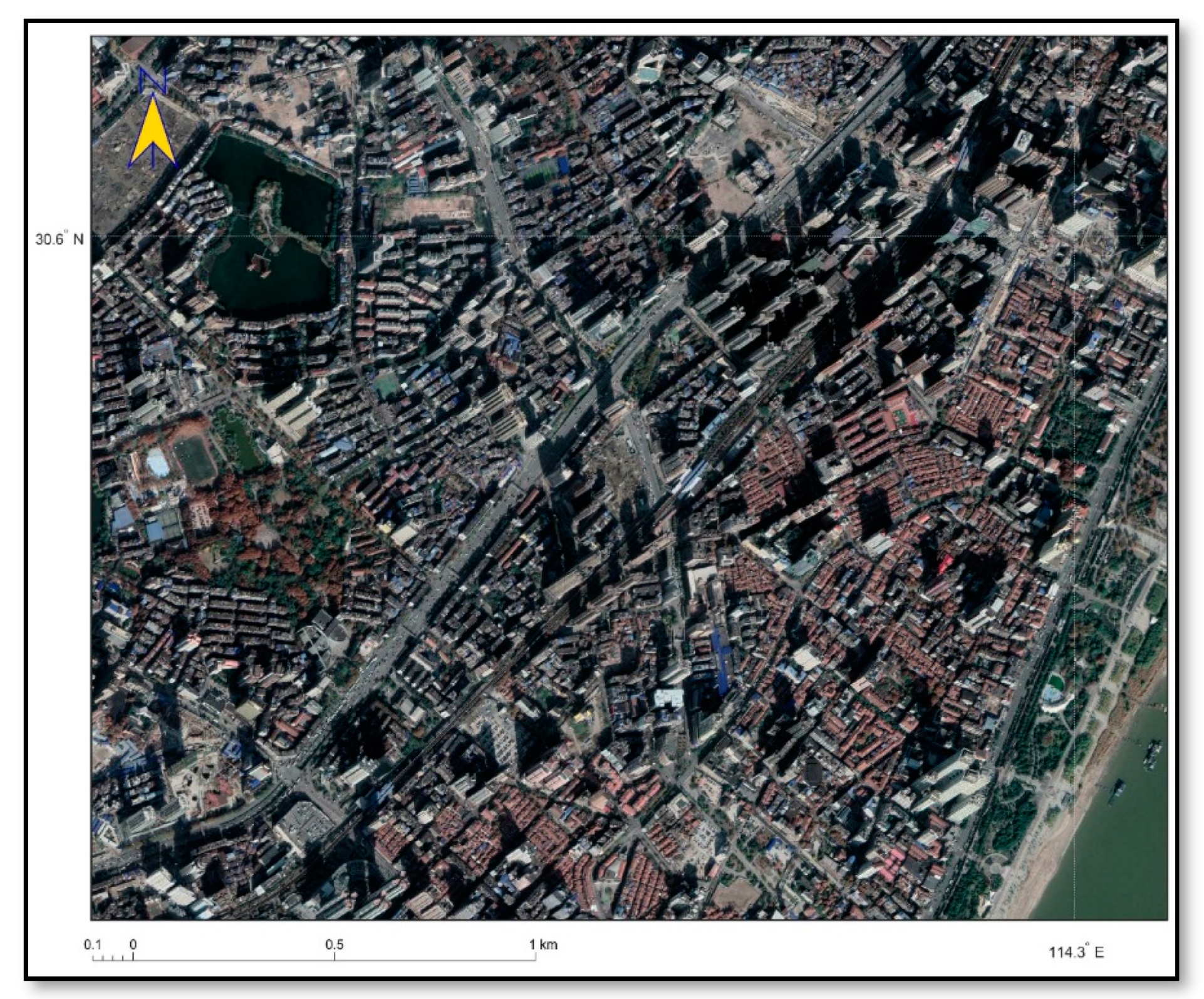
The study area considered the southwestern corner of Jiang’an District, Wuhan, Hubei Province, China. This area is under the jurisdiction of the Qiuchang Street Police Station, comprises approximately 7.5 km2 (30°58′ N–30°60′ N, 114°27′ E–114°30′ E) and has a registered population of 222,413 inhabitants. All data (i.e., crime records, building boundaries, and household records) were obtained from the Police Geographical Information System of the Wuhan Public Security Bureau.
The study area belongs to the old city of Wuhan and is a typical urban commercial and residential area. There are high- and medium-grade commercial units in the area, along with construction sites and several farms. The layout of the area is relatively complicated, and the number of crimes, especially burglary, is high. Figure 1 shows the satellite image of the study area.
After organizing the burglary data provided by the Police Geographical Information System, we located the 392 burglary cases over 7 consecutive months from 1 January 2013 to 30 July 2013 in the study area (Figure 1). Hence, 56 crimes were committed per month on average, with a standard deviation of 2.797. Each datapoint includes the geographic location and time of the crime (usually the time of reporting to the police accurate up to a daily scale).
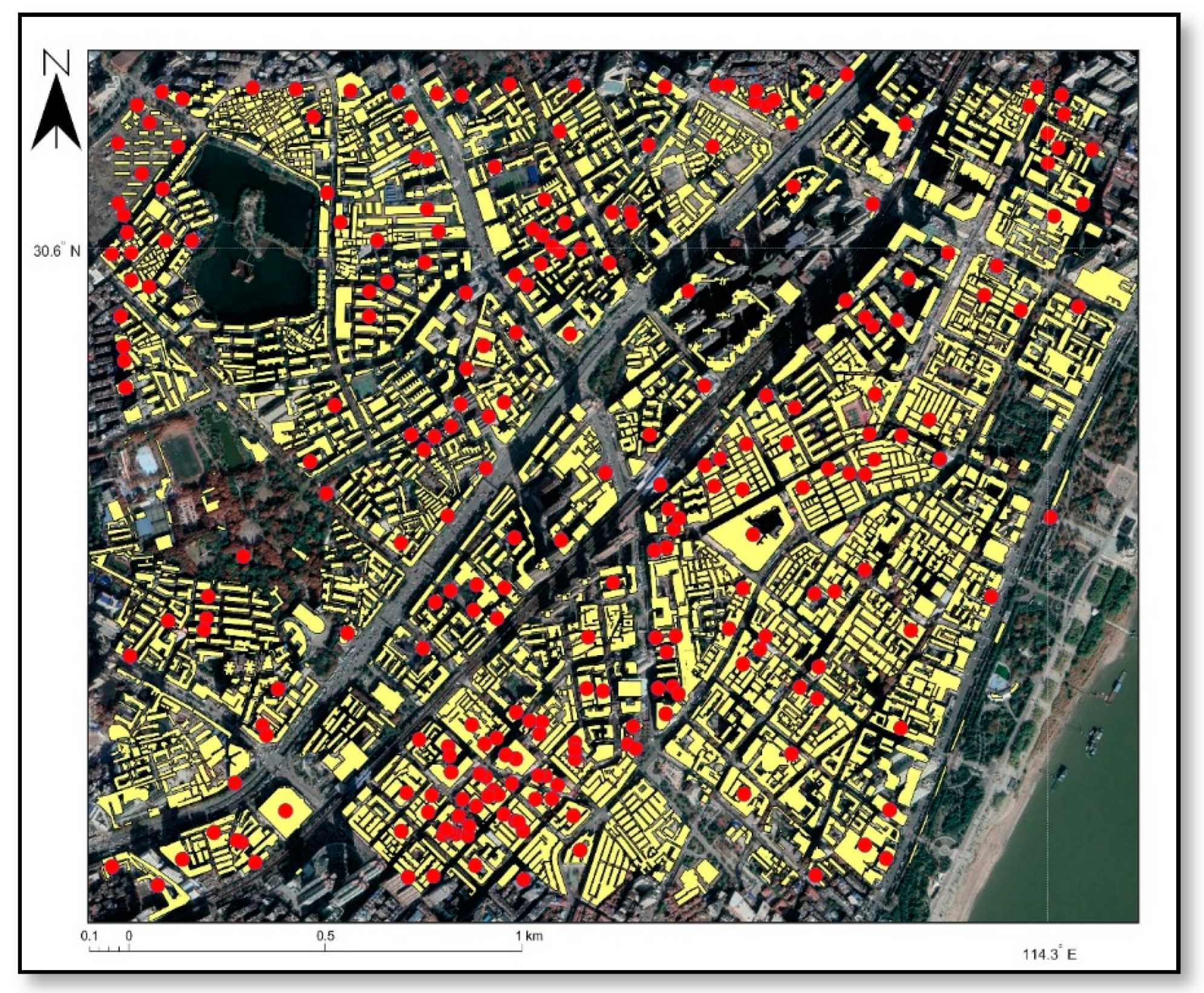
The geographic units (i.e., buildings) used as spatial constraints in this study are described by its boundary vector data. To calculate the crime risk at each type of building in the study area, it is necessary to independently determine its social indicators and environmental factors. Table 1 summarizes the data used in this study. Figure 2 illustrates the burglary cases and geographic units defined by building boundaries in the study area.
3.2. Similarity Measurement of Environmental Factors
To introduce differences of buildings into the traditional diffusion model, it is necessary to understand the spatial distribution characteristics of social and environmental factors within the study area and then calculate the similarity between buildings in which burglary cases occurred and their surroundings. As different buildings have specific social environments, conditions for crimes also vary. Here, we refer to crime condition as external environmental factors required to turn a crime motivation into action (e.g., many targets for burglary). Due to the limited data, we consider household density as the only environmental factor of buildings in the study area.
3.2.1. Spatial Distribution of Environmental Factors
We use house boundary to constrain the space for burglary cases and household data, and to facilitate the determination of location, size, and household density, thus allowing for quantifying the social environment in buildings. In addition, the topological spatial relations [56] between house boundary and location are used to obtain environmental factors of specific geographic units. The household density per geographic unit can be calculated as:
where is the household density, is the number of households, and , are the number of floors and area, respectively, of geographic unit .
For setting geographic areas, we use grids corresponding to the latitude and longitude are with as the respective lengths:
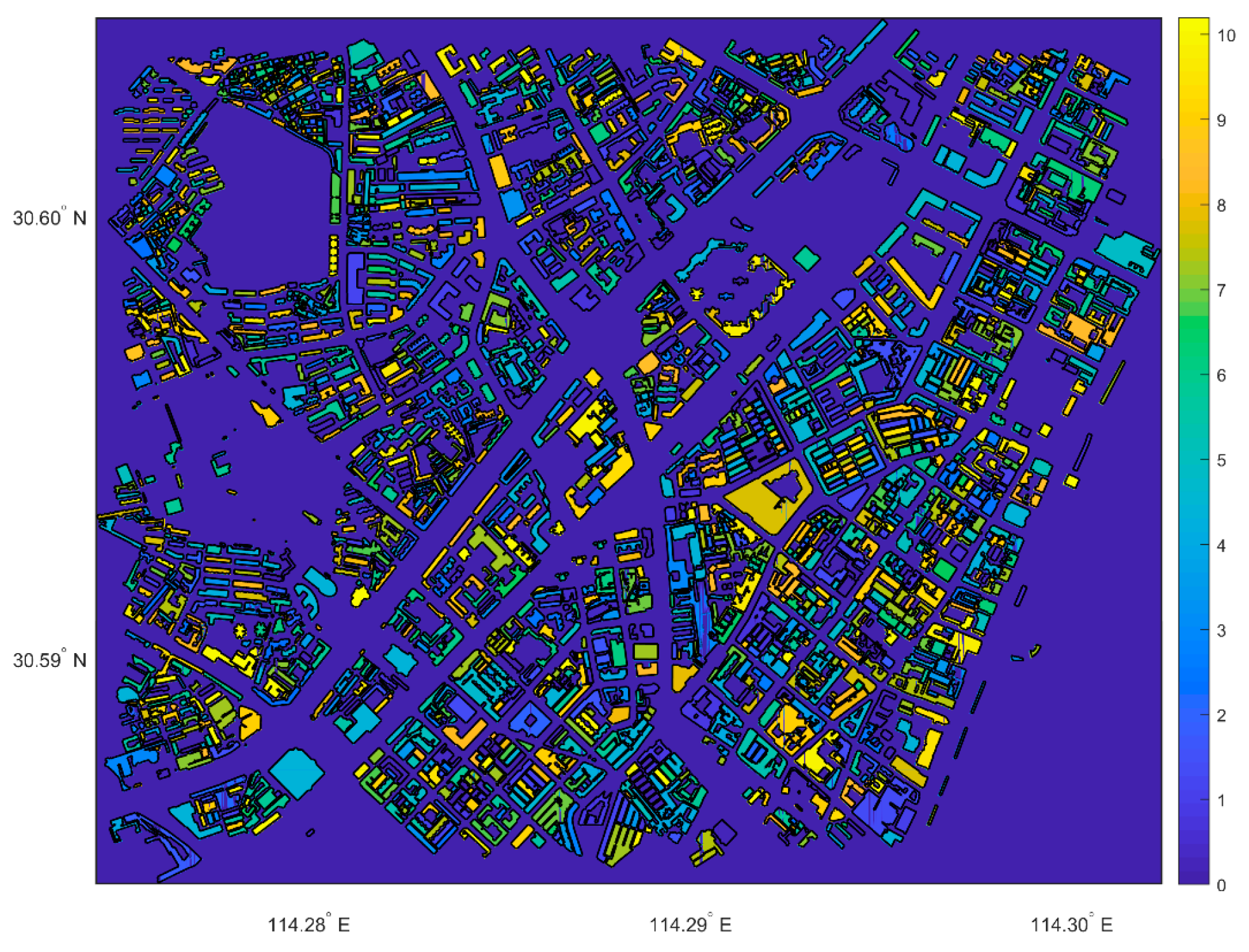
The grid lines divide the geographic space of the study area into cells, for which the density values are determined. The results of household density rasterization in the study area are shown in Figure 3, where . The household density in the study area ranges from large (yellow) to small (blue). The spatial distribution of household density is highly variable among buildings.
3.2.2. Similarity Measure
In machine learning and data mining, it is common to quantify the differences in samples to evaluate their similarity. The distance between feature vectors of samples is commonly used to determine similarity through methods including the Euclidean distance, Mahalanobis distance, cosine distance, Manhattan distance, and comentropy. To calculate the similarity of environmental factors between buildings in which burglary cases occurred and surrounding buildings, we assign a diffusion intensity of crime risk to surrounding buildings, and the similarity in the environmental factor (i.e., household density) between buildings is then determined.
Similarity is defined by the distance of household density in geographic units. The distance of household density from building (in which a burglary case occurred) to building is defined as:
where and are the household density of buildings and , respectively, is the dissimilarity of household density between the buildings, is a parameter controlling the decline of distance of the environmental factor with spatial distance, and is a parameter controlling the smoothness of the distance measure between buildings.
When a burglary case occurs in a building, the near-repeat theory indicates that the risk of a similar crime spreads to adjacent buildings and declines with increasing space and time distance [43]. Assuming that the similarity of environmental factors also affects the spatial distribution of crime risk, we consider the similarity measure among buildings in the study area to improve the prediction accuracy of the traditional diffusion model.
Specifically, when burglary occurs, the similarity between the building where it occurred and surrounding buildings is evaluated using Formula (2), and a distribution vector diagram of residence similarity is generated and rasterized to describe the spatial distribution of environmental factors with respect to the target building. For the vector diagram, we generate similarity distributions in all the buildings where burglary cases occurred.
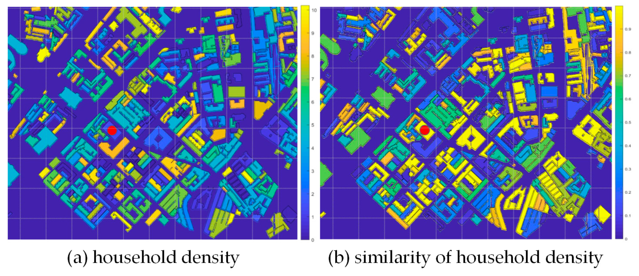
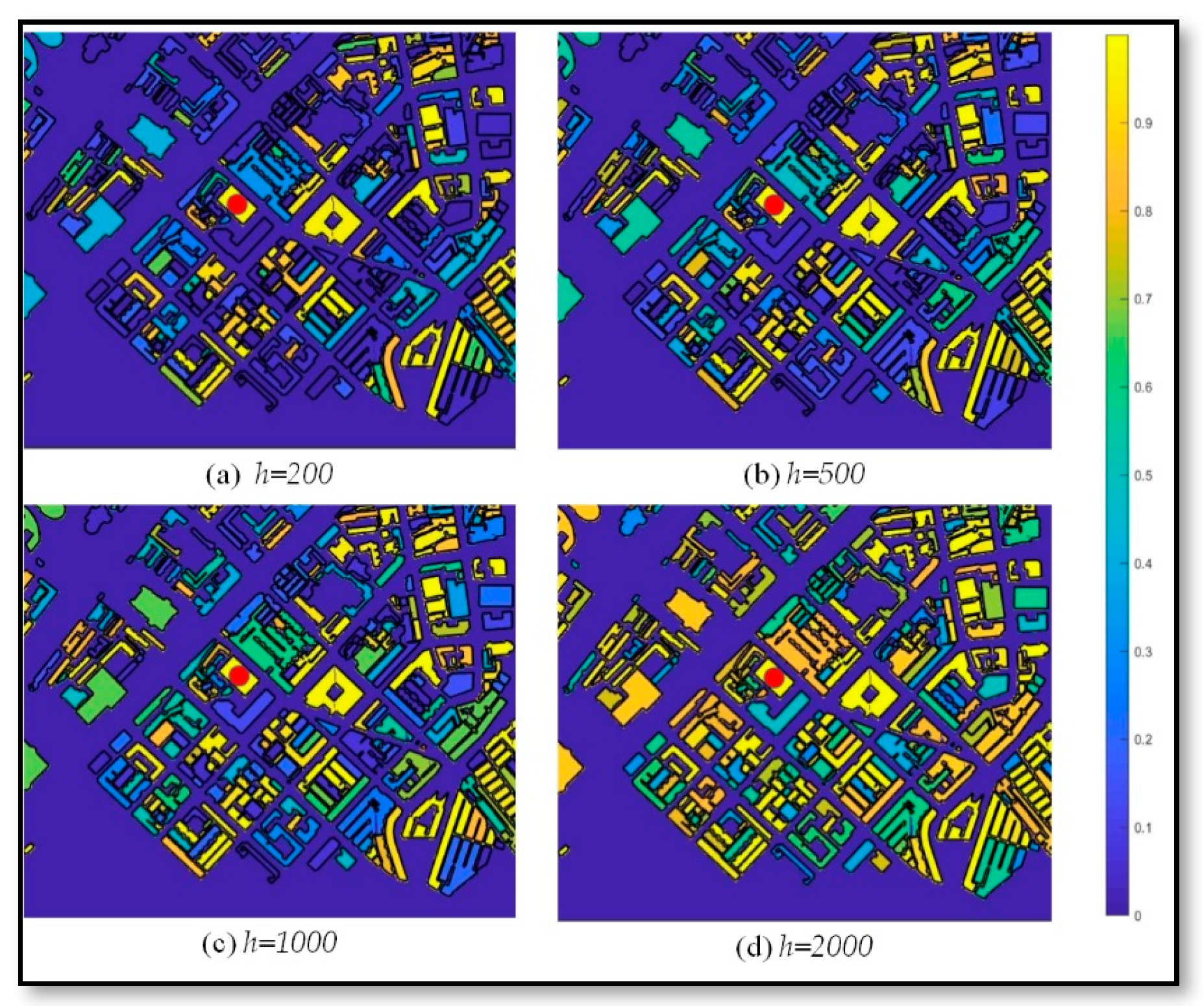
Figure 4a shows the spatial distribution of household density in the study area and crime cases marked with red dots. Figure 4b shows the spatial distribution of household density similarity between a building marked with red dot and the surrounding buildings with yellow and blue indicating high and low similarity, respectively. The similarity is clearly low regarding environmental factors between the target and surrounding buildings. The spatial distribution of similarity, , is generated by case , which after rasterization, is regarded as a binary function of the spatial distribution of similarity between buildings for this case. Figure 5 shows the influence of parameter on the similarity between geographic units. Figure 5 shows that higher parameter implies higher similarity between geographic units.
3.3. Diffusion Model
In this section, we focus on the motivation and process of using environmental similarity to construct the proposed anisotropic diffusion model (AnisDM).
3.3.1. Diffusion Coefficient Function
The AnisDM is widely used in digital image processing [57,58] for tasks such as image denoising, restoration [57], and segmentation [58]. Unlike the traditional diffusion model [13,42,50] with constant diffusion coefficients, the AnisDM allows a variable diffusion rate per grid cell in a geographic area. The AnisDM is given by:
where is the divergence operator, and respectively represent the gradient operator and Laplace operator, is a diffusion coefficient function, which is a function of the image gradient in image processing and usually designed according to two conditions: (1) intensify the diffusion coefficient in the smooth and homogeneous areas of the image grayscale value to reduce noise, and (2) weaken the diffusion coefficient in edges, textures, and other areas of the image to preserve features.
Different from the traditional isotropic diffusion models, by using diffusion coefficient function , the AnisDM controls the diffusion efficiency of pixels in different spatial positions in the image and varies the diffusion rate of pixels in different spatial grayscale values. Based on this concept, we improve the traditional diffusion model [43] by combining the diffusion coefficient function with environmental factors of the geographic units at crime locations.
Specifically, we use the diffusion coefficient function to describe the transmission of crime (burglary) risk in a specific area and environment. Based on [59], we propose the following diffusion coefficient function considering spatiotemporal and environmental distance:
The functions with subscript indicate the relationship between current building i (in which a burglary case occurred) and surrounding building . Function is the spatiotemporal and environmental distance between buildings , and weighs spatial distance coefficient and environmental similarity coefficient . The weight between the spatial and environmental distances is balanced by parameter . In addition, describes the spatial distance between buildings.
3.3.2. Proposed AnisDM
To better understand the spatiotemporal distribution of crime risk, we analyzed the distribution transference considering the spatial coordinates of crime cases. Then, we devised a method to include environmental factors, which distinguish geographic units in the study area, for predicting the spatiotemporal dynamics of crime risk. The diffusion coefficient function is used to describe the influence of environmental factors on the spatial distribution of crime risk by setting the diffusion rate per grid cell.
When case occurs in building , similarity between the household density of building and building is calculated, and the corresponding diffusion coefficient function is generated. An intuitive way to understand this is to consider the environmental difference between buildings and for places of crime occurrence to establish a crime sensitivity according to the degree of similarity, and then integrate the calculation into the model for diffusion.
The proposed AnisDM is given by:
where represents the dynamic process of crime (burglary) risk caused by crime in geographic area . Formula (9) is the overall distribution of crime risk, in Equation (10) is the diffusion coefficient function of crime risk generated by case, and is the initial distribution where indicate the initial risk caused by case . Equations (11) and (12) are Dirichlet boundary conditions.
For case , its risk value is introduced through initial distribution . The parameters can be determined by a spatiotemporal diffusion distance (e.g., considering 400 m and 28 days) of risk values obtained by near-repeat analysis combined with the size of the grid and cells and the timestep. Beyond a spatiotemporal distance threshold, the risk value falls below 20% of the initial value, reaching a level at which hotspot policing does not need to be carried out. Then, a crime risk below 20% means that the probability of burglary is only 20% higher than the average, where 20% is an empirically chosen value determined by the user (e.g., police officer), and this rate does not obviously appear on the map.
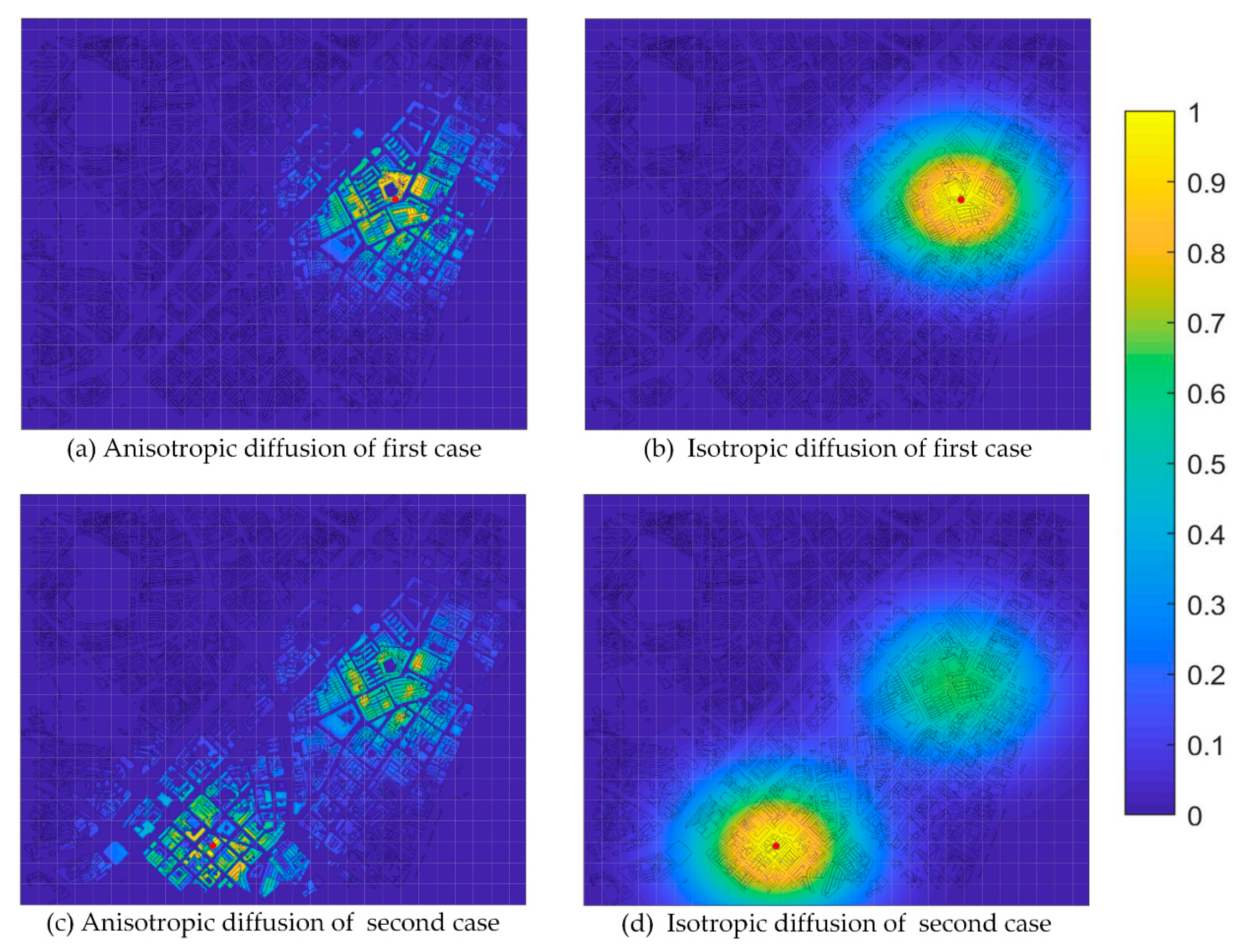
Two burglary cases from January 2013 are illustrated in Figure 6. The cases were located at 30°5958′ N, 114°2953′ E and 30°5877′ N, 114°2851′ E, and occurred over a period of 8 days. According to the near-repeat theory [37,38], these two cases change the spatial distribution of local crime risk in the area where they occurred, as crime risk spreads from its origin to the surroundings. The level of crime risk indicates where hotspot policing is necessary and its specific space–time and range. Figure 6a,b respectively show the test results of anisotropic and isotropic diffusion, where crime risk of the surrounding buildings obtained from the IsotDM only considers spatiotemporal distance, whereas that obtained from the AnisDM also considers the similarity between buildings and household density around the case location. Figure 6c,d show the spatial distribution of crime risk 1 week after the second case occurred, where the local crime risk caused by the first case has dropped to less than 50%.
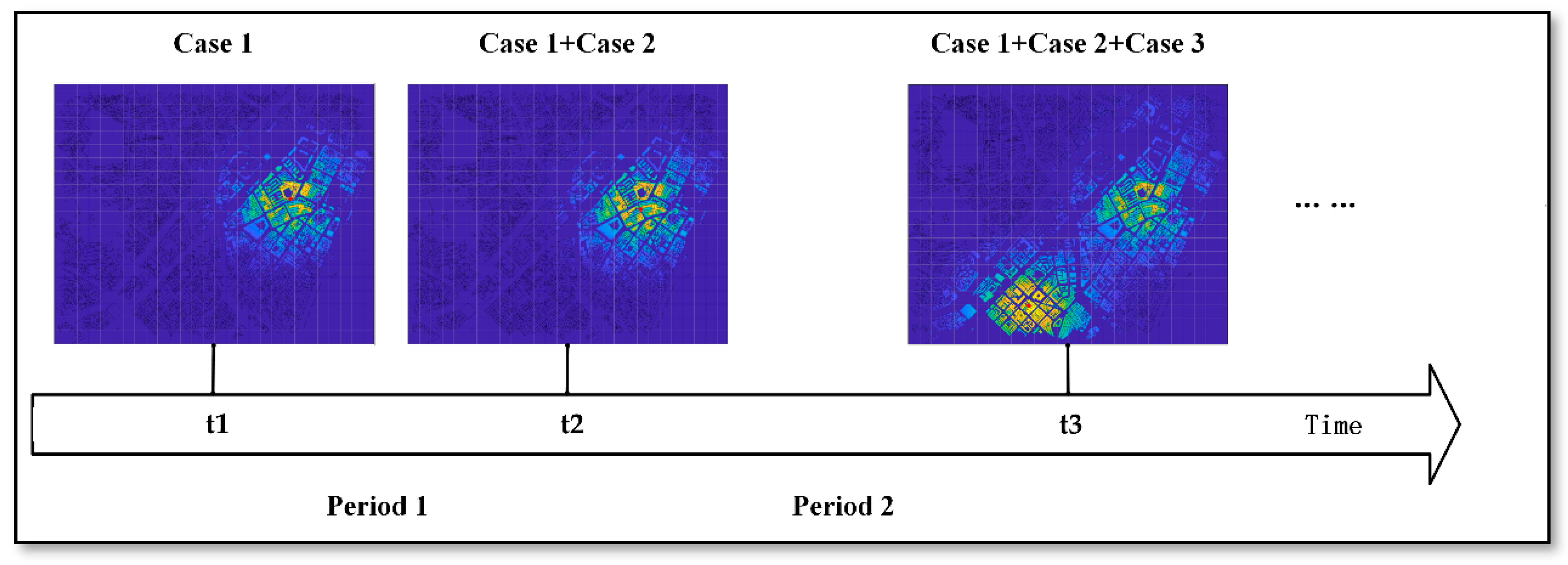
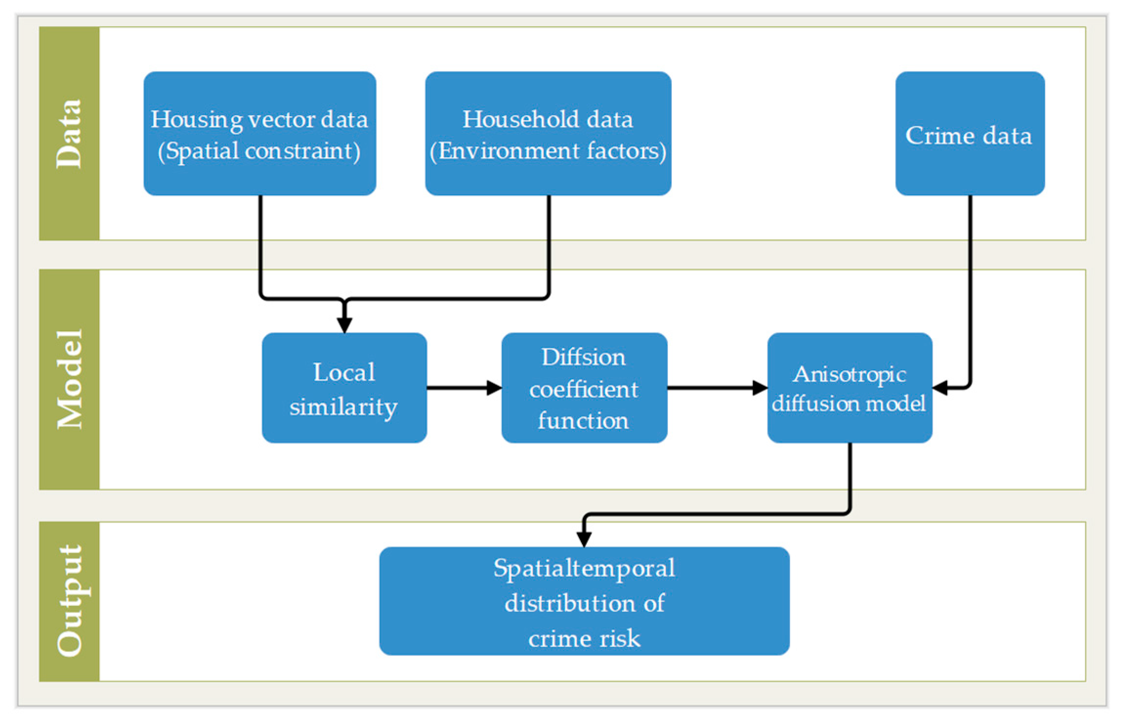
To calculate the spatiotemporal transmission of crime risk caused by case in chronological order, all burglary cases should be input into Formula (8). Then, through Formula (9), the processes are superimposed according to chronological order, as illustrated in Figure 7, where the time interval is 1 day between cases 1 and 2, and 3 days between cases 2 and 3. By inputting the crime risk caused by burglary into the diffusion model described by Formula (8) and overlaying each case according to the time interval of case occurrence, the overall spatiotemporal distribution of crime (burglary) risk is finally obtained. The flowchart of the proposed crime prediction algorithm is shown in Figure 8.
4. Experiment, Results and Discussion
To verify the effectiveness of the algorithm in this study, we used real data to verify the proposed prediction method. The study area comprises the interior of Jiangan District, Wuhan City, Hubei Province, China. A computer with Core i7 4770MQ processor, GTX765m GPU, and 8 GB memory was employed to run the algorithms implemented on MathWorks’ MATLAB 2016 and Python 3.6 (including GeoPandas, PySAL, and other open source tools of geographical information processing). The test area was of approximately on a grid of cells, and thus the area represented by a single cell was approximately .
There are 2428 housing vector datapoints in the test area. The housing vectors provide spatial constraints for the crime cases and household data, and allow determining the accuracy of crime prediction at building scale. There is a registered population of 222,413 inhabitants in the study area. The number of cases is 392 over a time span of 7 months (January to July, 2013), with an average of 56 cases per month, standard deviation of 21.54, and range of 55. The month with the largest number of cases was May with 72 cases, and that with the least cases was February with 17 cases.
We used results from [20] to set the spatiotemporal distance of crime risk transmission for the model in this study, obtaining values of 400 m and 28 days. The initial value of crime risk was set to 0.94. Moreover, the grid cells with the top 10% crime risk values were regarded as areas requiring hotspot policing.
For implementing the method, we considered the following parameters in the AnisDM:
are indices of geographic units, and is a collection of geographic units, ;
is the case index, and is number of cases, ;
is a time index of burglary cases. We divided criminal cases into parts by month, ;
is the similarity of household density values between buildings and ;
is the initial distribution of crime risk caused by case , ;
is used to control the smoothness of environmental distance between different buildings, which was set to 1000;
is the number of geographic units in the study area, being 2428 in this study;
and are the space steps between latitude and longitude, respectively, which are approximately 1 m;
and are the number of grids longitudinally and latitudinally, where and ;
is used to control the weight between spatial and environmental distances, which was set to 0.5 in this study.
4.1. Crime Prediction Results
To verify the effectiveness of the AnisDM for crime prediction, we used the attributes of incident time per burglary case and divided the datapoints from January until July, 2013 to employ the model in a monthly basis. By analyzing the spatial distribution of burglary risk at the -th month and comparing the real distribution of burglary cases at the ()-th month, we evaluated the effectiveness of the AnisDM on crime prediction. In addition, we considered monthly data to conveniently analyze the prediction accuracy. Still, the proposed method can be iterated in a case basis and generate the corresponding results (see Figure 7), thus being suitable for real-time application.
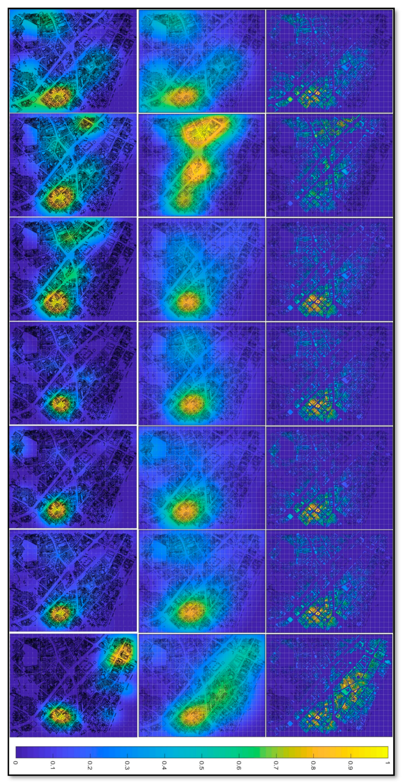
For comparison, we evaluated crime prediction using the IsotDM and spatial KDE (Kernel Density Estimation) [43,44]. The first column of Figure 9 shows the results obtained from the spatial KDE from January to July. The second column shows the results obtained from the IsotDM, and the third one shows the results obtained from the proposed AnisDM over the study area. Overall, the spatial distribution of crime risk predicted using the proposed AnisDM is similar to that using the IsotDM, and spatial KDE is different from them because it is time independent. The main hotspots of crime risk are clustered around the spatiotemporal points of burglary case occurrences. The most notable difference between the two crime prediction methods is the detailed crime prediction of hotspots at the building level obtained from the proposed AnisDM. Compared to the IsotDM, the AnisDM specifies the degree of risk at different buildings in the hotspot areas. In the following, we provide a quantitative analysis of the test results through various indices.
4.2. Crime Prediction Accuracy
We assessed the accuracy of spatiotemporal distribution of burglary cases forecasted by the IsotDM and AnisDM using the prediction accuracy index (PAI) [10,60], which requires using high-risk regions over small areas to evaluate more cases of crime prediction. The general expressions of PAI is given by:
where is the value of cases located in crime risk hotspots upon determination (generally, the grid cells with the top 10% of crime risk is deemed as hotspot) and allows for forecasting the correct case number, is the number of predicted crime cases, is the area of crime risk hotspots upon determination, and is the study area.
We divided the study area into different regions according to crime-risk values estimated by the IsotDM and AnisDM (grid cells with 0.5%, 1%, 5%, and 10% of the crime risk ranking), and then the prediction hit rate and PAI of each model in these regions were calculated to assess crime prediction effectiveness [10,60]. Although the hotspot distribution and risk values of crime obtained from the two models vary, uniformly selecting high-risk areas in proportion can effectively reduce the variation among crime prediction models during estimation. Therefore, the PAI can be used to intuitively compare the prediction effectiveness of the models [60].
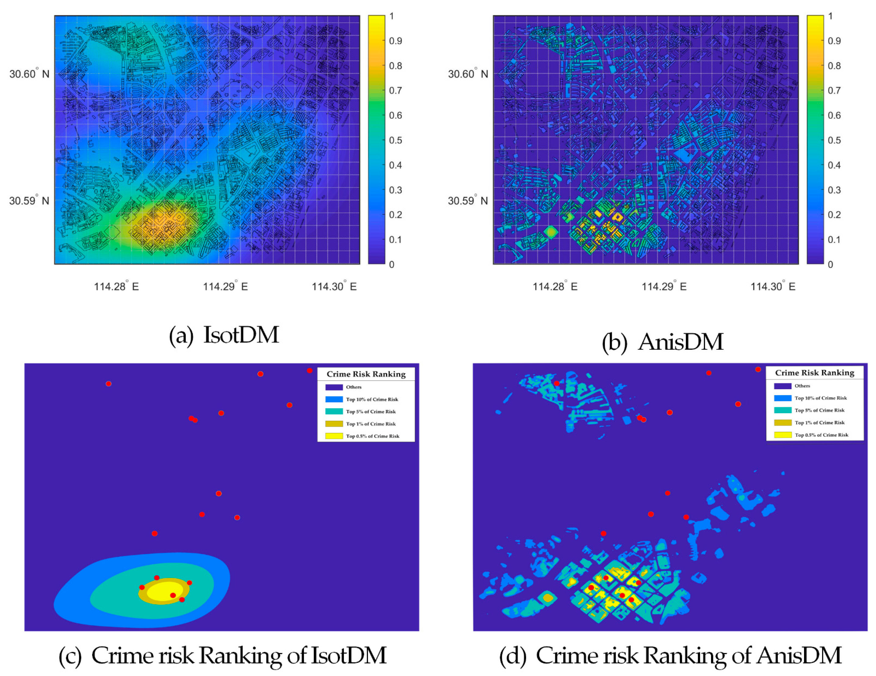
The performance of crime prediction using the IsotDM and AnisDM is shown in Figure 10 considering burglary case data from January, 2013. In addition, data from February was used for overlay analysis with the crime risk map for a deeper comparison between crime prediction results. The location of crime risk hotspots forecast by the IsotDM and AnisDM is similar (centered on the lower-left region of the study area), but the crime risk distribution varies greatly in local details, both in space and scope. The PAI of the IsotDM and AnisDM is shown in Figure 10c,d, respectively. Figure 10d shows that five cases with crime risk estimated through the AnisDM are among the top 0.5% in ranking with PAI of 58.823, and five cases are among the top 1% in ranking with PAI of 29.411. Moreover, six cases are among the top 5% in ranking with PAI of 7.058, and six cases are among the top 10% in ranking with PAI of 3.529.
4.3. Crime Prediction Comparison and Analysis
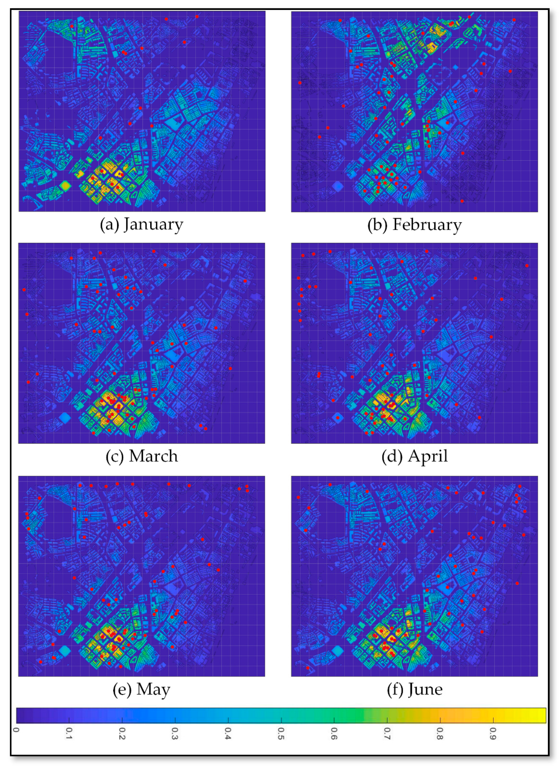
Here, we describe the calculation of prediction correctness for four types of crime risks (i.e., top 0.5%, 1%, 5%, and 10% crime risk values) obtained from the spatial KDE, IsotDM and AnisDM. In addition, an overlay analysis is conducted for crime cases from February to July on a monthly basis considering the last stage of crime risk distribution and different crime risk areas for the AnisDM. Figure 11a–f show the crime prediction using the AnisDM and cases from January to June, with the crime data from February to July being overlaid on the corresponding maps. The overlapping degree of crime prediction in February with the crime data in March shows low potential criminality, maybe by the occurrence of a massive event called Spring Festival. Compared with other months, the number of crime cases in February is low, being only 17, which is much less than the average of 56 cases per month. Apart from these months, crime prediction results are similar among consecutive months, and crime prediction is accurate.
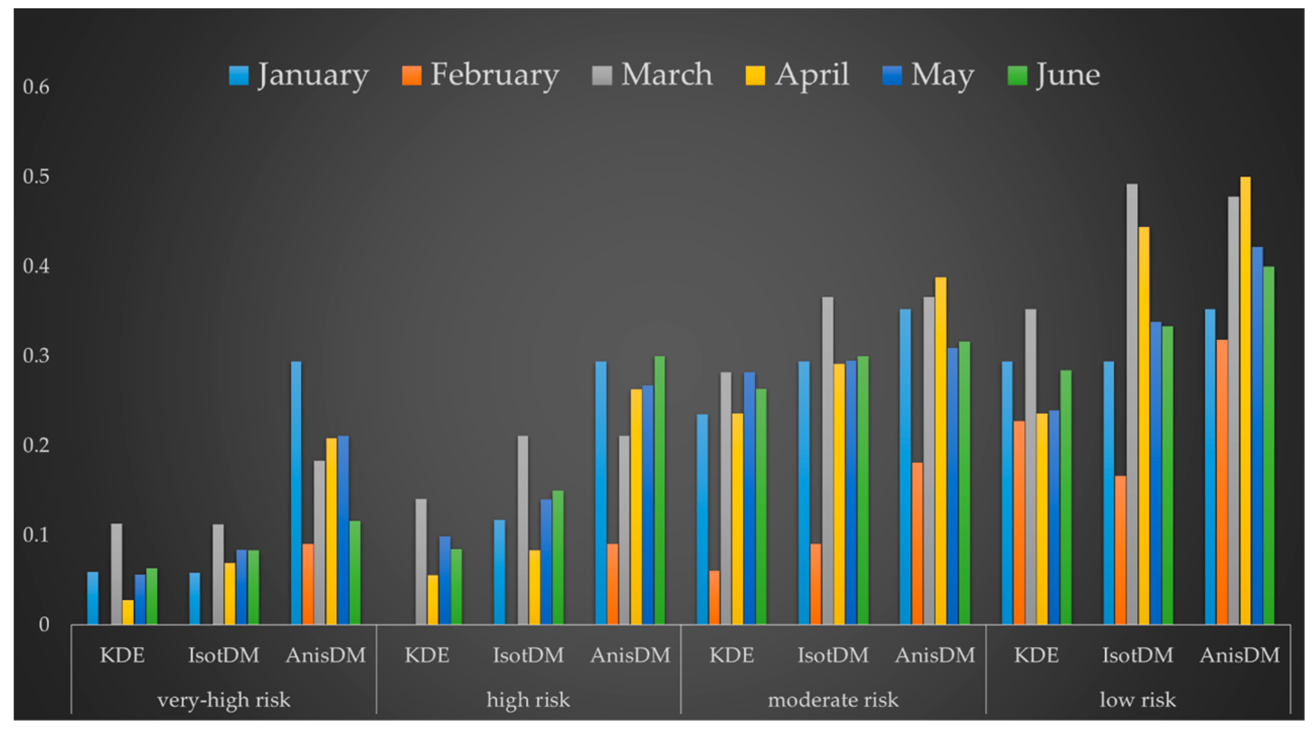
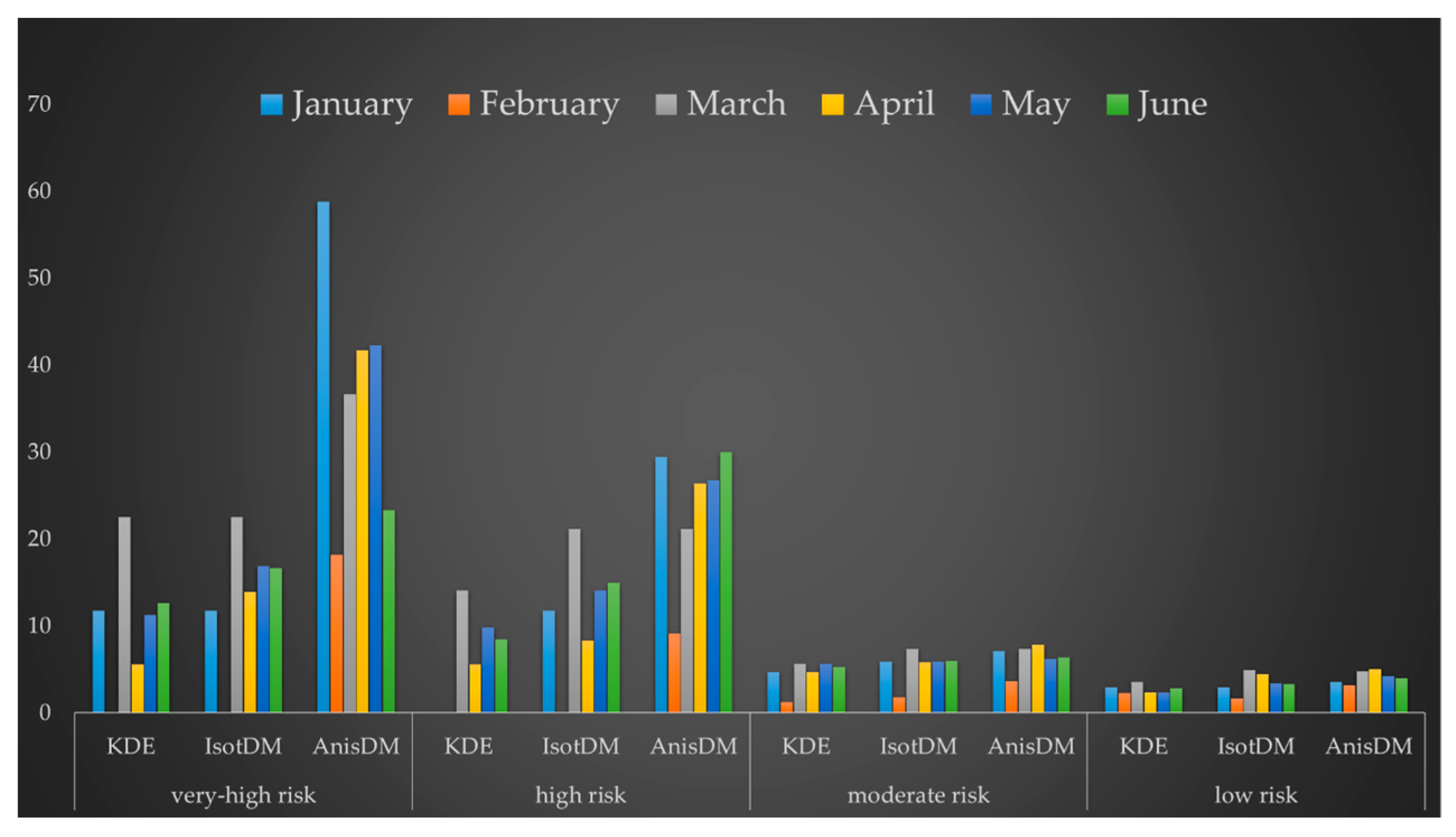
Then, we compared the PAIs from all the results to quantify and analyze the prediction effect of the spatial KDE, IsotDM and AnisDM. We labeled the four types of crime risks, namely, 0.5%, 1%, 5%, and 10%, as very-high, high, moderate, and low risk, respectively. We predicted the number of burglary cases over the following month in the study area considering these four types of crime risks. Then, we calculated the PAI and hit rate and performed comparisons for each of the 6 evaluated months. The resulting hit rate and PAI are shown in Figure 12 and Figure 13, respectively.
The hit rate of the AnisDM is greater than or equal to that of the IsotDM and spatial KDE, especially for very-high and high risk. In fact, the IsotDM has average hit rate of only 6.8% and 11.7%, with average PAI of 13.62 and 11.71 for very-high and high risk, respectively, and the PAI of spatial KDE even lower with average of 10.6 and 6.3, whereas the AnisDM algorithm has average hit rate of 18.4% and 23.8%, with average PAI of 36.81 and 23.79, respectively. Thus, the prediction performance of the AnisDM is 170% and 103.5% above that of the IsotDM. Hence, nearly one fifth of burglary cases in the next month occur in a geographic space that covers only 0.5% or 1% of the research area. If key policing and surveillance is carried out in this region, there is a chance of achieving better crime prevention while saving manpower and financial resources. For moderate and low risk, the difference between the prediction performance of the two models gradually reduce. The hit rate of the IsotDM algorithm is 27.31% and 34.49% with PAI of 5.46 and 3.45 for moderate and low risk, respectively, and that of the AnisDM is 31.93% and 41.20% with PAI of 6.38 and 4.12, respectively. Therefore, the prediction performance of the AnisDM only increases by 16.9% and 19.5% compared to that of the IsotDM at the respective levels. Hence, as crime risk decreases, the prediction effect of the AnisDM gradually approaches that of the IsotDM. This is because the theoretical basis of the AnisDM is consistent with that of the IsotDM, and both are based on the near-repeat theory. Still, the AnisDM considers environmental similarity of geographic units where crimes occurred, providing more detailed crime prediction than the IsotDM.
The IsotDM simply conducts smoothing and diffusion of crime risk per grid cell in the study area in order to determine the spatiotemporal evolution of crime described by the near-repeat theory, but neglects social and environmental factors of the different geographic units where cases occur. By using the diffusion coefficient function to describe environmental factors at a building level in the study area, the proposed AnisDM extends the diffusion model based on the near-repeat theory by considering the correlation between the spatial distance and crime rate related to different environmental factors to improve crime prediction [34,35,61,62,63].
4.4. Sensitivity Analysis
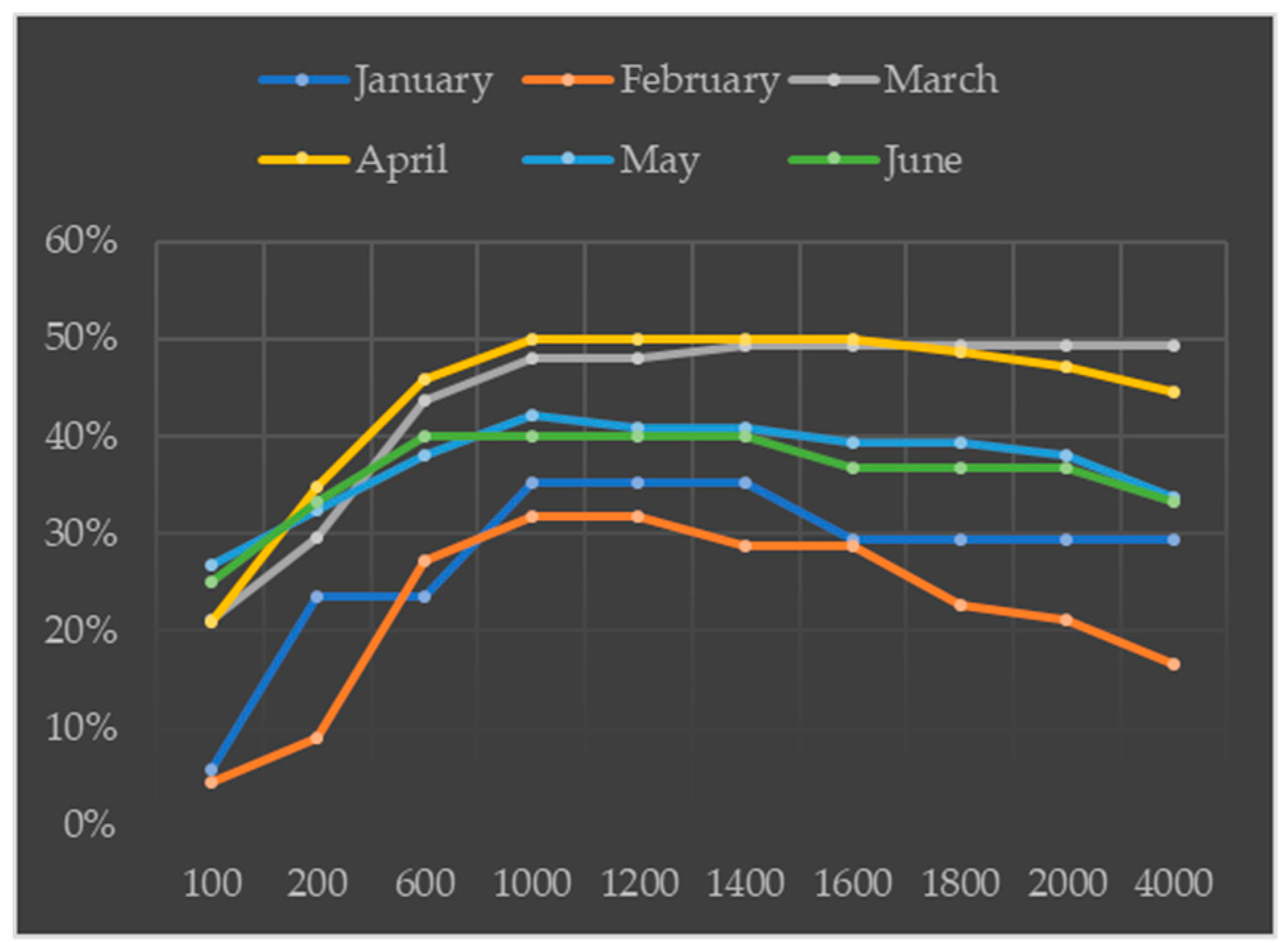
In the AnisDM, parameters and have great influence on the output. Hence, we analyzed the sensitivity of these parameters by changing their values and observing their influence on the prediction results.
Parameter controls the smoothness of the environmental similarity between different buildings. Hence, larger values imply higher similarity between buildings. For , the analysis results are shown in Figure 14, where the x and y axes depict parameter and the prediction accuracy, respectively, under extremely low risk (geographic area containing the top 10% grid cells of crime risk). For , the environmental similarity between buildings is extremely low, resulting in deficient crime prediction. For values of approximately 1000, the prediction accuracy reaches its maximum, and further increasing of parameter makes the accuracy to gradually decrease. In fact, increasing h beyond the maximum accuracy causes the AnisDM to degenerate into the IsotDM.
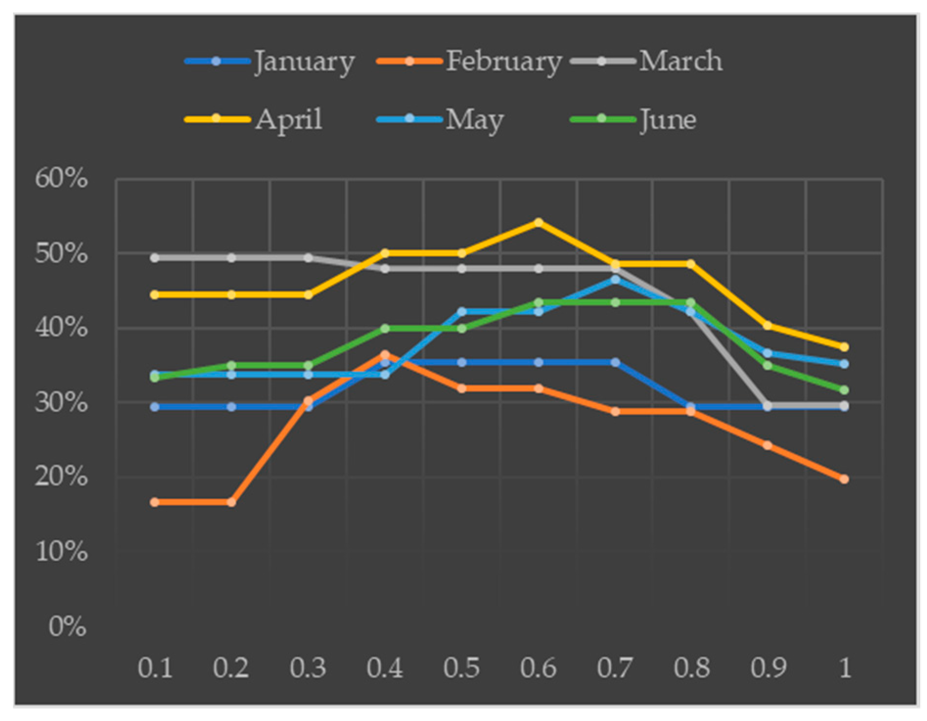
Parameter weighs the spatial and environmental distances of the diffusion coefficient function in the AnisDM. Hence, larger values imply higher correlation between crime prediction and environmental similarity. For , the prediction accuracy of the AnisDM is shown in Figure 15, where the x and y axes depict parameter and the prediction accuracy, respectively, under extremely low risk. For , the diffusion coefficient function mainly assigns the crime risk value to the surrounding buildings based on the spatiotemporal distance. Consequently, the AnisDM degenerates into the IsotDM, which only considers the spatial distance. For , this parameter has a substantial influence on crime prediction, reaching the maximum accuracy between 0.4 and 0.8 (we used to obtain the results in previous sections). Further increasing makes the prediction accuracy to gradually decrease. In fact, excessive values lead the model to only consider environmental factors for prediction, thus neglecting the location of crimes and undermining diffusion and prediction accuracy.
5. Conclusions
Based on the near-repeat theory, we propose the AnisDM for crime (specifically burglary) prediction. First, we determine environmental factors from buildings and their similarity in the study area to quantify environmental factors among buildings. Then, the diffusion coefficient function of the AnisDM combines the environmental factors with crime case locations to quantify the sensitivity of different buildings to crime. Finally, spatiotemporal dynamics are included in the diffusion model to predict crime as suggested by the near-repeat theory. Experimental results verify the advantages of the AnisDM compared to the traditional IsotDM regarding detailed crime prediction at building level to determine specific policing hotspots, which can provide support to deploy law enforcement.
Some limitations of the proposed method remain to be addressed. A gap remains between the crime prediction and application by the police. Due to data sensitivity, the quantity of environmental factors available for analysis is limited to household density, and reliable data on other factors are difficult to collect. Consequently, crime prediction accuracy has not reached a desired level for real-world application. In addition, parameter optimization should be considered to achieve the best prediction results. Although we have explored the gradient descent method and other optimization methods to find the optimal parameters, the non-convexity of the problem impedes achieving good results. Thus, we are currently selecting parameters based on our experience, but still investigating formal optimization methods [64]. Furthermore, the special combination of parameters may lead to the blow-up behavior in the solution of the diffusion model (i.e., the prediction results deviate greatly from the true value). Although the occurrence of this behavior is rare, it is worth of attention.
In future work, we will focus on several improvements to the proposed method. Specifically, we will consider how to use global optimization to obtain the optimal parameters. In addition, we will collect more data related to residential burglary for covering the following factors: economy (e.g., quantity and density of commercial buildings, such as stores, supermarkets, and commercial centers, and house pricing), geographical factors (e.g., density of high- and low-rise buildings, urbanization), population (e.g., number of permanent residents and migrants, rate of rental households, rate of private households, unemployment rate), nature of land utilization (e.g., road, residential, commercial, industrial zones, settlement places, public facilities), and risk factors (e.g., distribution of security cameras and police offices in communities). These data can be directly associated with surface geographic entities. Furthermore, we will consider the integration method between different environmental factors. We plan to use geographically weighted regression to analyze the correlation between different environmental factors and crime rates. With more detailed environmental factors per geographic unit, we believe that the crime prediction accuracy can be further improved. Finally, research shows that network-based crime prediction substantially outperforms the grid-based approach in terms of accuracy [64], and hence, we will apply road network data [65,66] to the diffusion model to further improve prediction.
Author Contributions
Conceived and designed the experiments: Yicheng Tang, Xinyan Zhu and Wei Guo. Performed the experiments: Yicheng Tang., and Wei Guo. Analyzed the data: Yicheng Tang. and Yaxin Fan. Wrote the paper. Ling Wu. updated the manuscript.
Funding
This research was funded by the National Key R&D Program, grant number 2018YFB0505500 and 2018YFB0505503; the National Natural Science Foundation of China, grant number 41830645, LIESMARS (State Key Laboratory of Information Engineering in Surveying, Mapping and Remote Sensing, Wuhan University) Special Research Funding, Research on key techniques of dynamic map with position-perceived and Social Geographic Computing Theory and Software Platform (Key Open Fund, LIESMARS), and Fundamental Research Funds for the Central Universities.
Acknowledgments
We gratefully acknowledge the anonymous reviewers for their insightful comments on the manuscript.
Conflicts of Interest
The authors declare no conflict of interest.
References
- Ye, X.; Wu, L. Analyzing the dynamics of homicide patterns in Chicago: ESDA and spatial panel approaches. Appl. Geogr. 2011, 31, 800–807. [Google Scholar] [CrossRef]
- Sherman, L.W.; Gartin, P.R.; Buerger, M.E. Hot Spots of Predatory Crime: Routine Activities and the Criminology of Place. Criminology 2010, 27, 27–56. [Google Scholar] [CrossRef]
- Farrell, G.; Pease, K. Once Bitten, Twice Bitten: Repeat Victimisation and Its Implications for Crime Prevention; Police Research Group Crime Prevention Unit Paper; Paper No. 46; Home Office Police Department: London, UK, 1993. [Google Scholar]
- Boni, M.A.; Gerber, M.S. Automatic Optimization of Localized Kernel Density Estimation for Hotspot Policing. In Proceedings of the IEEE International Conference on Machine Learning and Applications, Cancun, Mexico, 18 December 2017; pp. 32–38. [Google Scholar]
- Chiu, S.T. A comparative review of bandwidth selection for kernel density estimation. Stat. Sinica 1996, 6, 126–145. [Google Scholar]
- Turlach, B.A. Bandwidth Selection in Kernel Density Estimation: A Review. CORE Inst. Statist. 1993, 23–493. [Google Scholar]
- Kennedy, L.W.; Caplan, J.M.; Piza, E. Risk Clusters, Hotspots, and Spatial Intelligence: Risk Terrain Modeling as an Algorithm for Police Resource Allocation Strategies. J. Quant. Criminol. 2011, 27, 339–362. [Google Scholar] [CrossRef]
- Gorr, W.; Olligschlaeger, A.; Thompson, Y. Short-term forecasting of crime. Int. J. Forecast. 2003, 19, 579–594. [Google Scholar] [CrossRef]
- Gerber, M.S. Predicting crime using Twitter and kernel density estimation. Decis. Supp. Syst. 2014, 61, 115–125. [Google Scholar] [CrossRef]
- Chainey, S.; Tompson, L.; Uhlig, S. The Utility of Hotspot Mapping for Predicting Spatial Patterns of Crime. Secur. J. 2008, 21, 4–28. [Google Scholar] [CrossRef] [Green Version]
- Mohler, G. Marked point process hotspot maps for homicide and gun crime prediction in Chicago. Int. J. Forecast. 2014, 30, 491–497. [Google Scholar] [CrossRef]
- Johnson, S.D. Repeat burglary victimisation: A tale of two theories. J. Exp. Criminol. 2008, 4, 215–240. [Google Scholar] [CrossRef]
- Short, M.B.; D’Orsogna, M.R.; Brantingham, P.J.; Tita, G.E. Measuring and Modeling Repeat and Near-Repeat Burglary Effects. J. Quant. Criminol. 2009, 25, 325–339. [Google Scholar] [CrossRef] [Green Version]
- Mohler, G.O.; Short, M.B. Geographic Profiling from Kinetic Models of Criminal Behavior. Siam J. Appl. Math. 2012, 72, 163–180. [Google Scholar] [CrossRef] [Green Version]
- Tang, Y.; Zhu, X.; Guo, W.; Ye, X.; Hu, T.; Fan, Y.; Zhang, F. Non-Homogeneous Diffusion of Residential Crime in Urban China. Sustainability 2017, 9, 934. [Google Scholar] [CrossRef]
- Law, J.; Quick, M. Exploring links between juvenile offenders and social disorganization at a large map scale: A Bayesian spatial modeling approach. J. Geogr. Syst. 2013, 15, 89–113. [Google Scholar] [CrossRef]
- Lee, J.S.; Park, S.; Jung, S. Effect of Crime Prevention through Environmental Design (CPTED) Measures on Active Living and Fear of Crime. Sustainability 2016, 8, 872. [Google Scholar] [CrossRef]
- Law, J.; Quick, M.; Chan, P. Bayesian Spatio-Temporal Modeling for Analysing Local Patterns of Crime Over Time at the Small-Area Level. J. Quant. Criminol. 2014, 30, 57–78. [Google Scholar] [CrossRef]
- Johnson, S.D.; Bowers, K.J. The Burglary as Clue to the Future: The Beginnings of Prospective Hot-Spotting. Eur. J. Criminol. 2004, 1, 237–255. [Google Scholar] [CrossRef]
- Ye, X.; Xu, X.; Lee, J.; Zhu, X.; Wu, L. Space-time interaction of residential burglaries in Wuhan, China. Appl. Geogr. 2015, 60, 210–216. [Google Scholar] [CrossRef]
- Hoppe, L.; Gerell, M. Near-repeat burglary patterns in Malmö: Stability and change over time. Eur. J. Criminol. 2018, 1203272670. [Google Scholar] [CrossRef]
- Bediroglu, G.; Bediroglu, S.; Colak, H.E.; Yomralioglu, T. A Crime Prevention System in Spatiotemporal Principles with Repeat, Near-Repeat Analysis and Crime Density Mapping: Case Study Turkey, Trabzon. Crime Delinq. 2018, 475245375. [Google Scholar] [CrossRef]
- Sturup, J.; Rostami, A.; Gerell, M.; Sandholm, A. Near-repeat shootings in contemporary Sweden 2011 to 2015. Secur. J. 2017, 31, 73–92. [Google Scholar] [CrossRef]
- Melo, S.N.D.; Andresen, M.A.; Matias, L.F. Repeat and near-repeat victimization in Campinas, Brazil: New explanations from the Global South. Secur. J. 2017. [Google Scholar] [CrossRef]
- Chen, P.; Yuan, H.; Li, D. Space-time analysis of burglary in Beijing. Secur. J. 2013, 26, 1–15. [Google Scholar] [CrossRef]
- Wells, W.; Wu, L. Proactive Policing Effects on Repeat and Near-Repeat Shootings in Houston. Police Q. 2011, 14, 298–319. [Google Scholar] [CrossRef]
- Rosenfeld, R.; Levin, A. Acquisitive Crime and Inflation in the United States: 1960–2012. J. Quant. Criminol. 2016, 32, 427–447. [Google Scholar] [CrossRef]
- Marie, O.; Machin, S.; Vujić, S. The Crime Reducing Effect of Education. Econ. J. 2011, 121, 463–484. [Google Scholar] [Green Version]
- Zhang, L.; Messner, S.F.; Liu, J. A multilevel analysis of the risk of household burglary in the city of Tianjin, China. Brit. J. Criminol. 2007, 47, 918–937. [Google Scholar] [CrossRef]
- Harrison, R.A.; Gemmell, I.; Heller, R.F. The population effect of crime and neighbourhood on physical activity: An analysis of 15,461 adults. J. Epidemiol. Community Health 2007, 61, 34–39. [Google Scholar] [CrossRef]
- Fazel, S.; Grann, M. The population impact of severe mental illness on violent crime. Am. J. Psychiat. 2006, 163, 1397–1403. [Google Scholar] [CrossRef]
- McCann, B.J. Contesting the Mark of Criminality: Race, Place, and the Prerogative of Violence in NWA’s Straight Outta Compton. Crit. Stud. Media Commun. 2012, 29, 367–386. [Google Scholar] [CrossRef]
- Malleson, N.; Andresen, M.A. The impact of using social media data in crime rate calculations: Shifting hot spots and changing spatial patterns. Cartogr. Geogr. Inf. Sci. 2015, 42, 112–121. [Google Scholar] [CrossRef]
- Liu, H.; Zhu, X. Joint Modeling of Multiple Crimes: A Bayesian Spatial Approach. ISPRS Int. J. Geo. Inf. 2017, 6, 16. [Google Scholar] [CrossRef]
- Liu, H.; Zhu, X. Exploring the Influence of Neighborhood Characteristics on Burglary Risks: A Bayesian Random Effects Modeling Approach. ISPRS Int. J. Geo. Inf. 2016, 5, 102. [Google Scholar] [CrossRef]
- Guerette, R.T. Analyzing Crime Displacement and Diffusion; Justice, U.D.O., Ed.; Center for Problem-Oriented Policing, 2009; Volume 10. Available online: http://www.popcenter.org/tools/displacement/print/ (accessed on 20 May 2019).
- Townsley, M.; Homel, R.; Chaseling, J. Infectious burglaries—A test of the near repeat hypothesis. Brit. J. Criminol. 2003, 43, 615–633. [Google Scholar] [CrossRef]
- Wells, W.; Wu, L.; Ye, X. Patterns of Near-Repeat Gun Assaults in Houston. J. Res. Crime Delinq. 2012, 49, 186–212. [Google Scholar] [CrossRef]
- Grubesic, T.H.; Mack, E.A. Spatio-temporal interaction of urban crime. J. Quant. Criminol. 2008, 24, 285–306. [Google Scholar] [CrossRef]
- Braga, A.A. The Effects of Hot Spots Policing on Crime. Ann. Am. Acad. Polit. Soc. Sci. 2001, 578, 104–125. [Google Scholar] [CrossRef]
- Townsley, M.; Homel, R.; Chaseling, J. Repeat Burglary Victimisation: Spatial and Temporal Patterns. Aust. N. Z. J. Criminol. 2000, 33, 37–63. [Google Scholar] [CrossRef] [Green Version]
- Mohler, G.O.; Short, M.B.; Brantingham, P.J.; Schoenberg, F.P.; Tita, G.E. Self-Exciting Point Process Modeling of Crime. Publ. Am. Stat. Assoc. 2011, 106, 100–108. [Google Scholar] [CrossRef] [Green Version]
- Short, M.B.; D’Orsogna, M.R.; Pasour, V.B.; Tita, G.E.; Brantingham, P.J.; Bertozzi, A.L.; Chayes, L.B. A statistical model of criminal behavior. Math. Mod. Meth. Appl. S 2008, 18, 1249–1267. [Google Scholar] [CrossRef]
- Zipkin, J.R.; Short, M.B.; Bertozzi, A.L. Cops on the Dots in a Mathematical Model of Urban Crime and Police Response. Discr. Cont. Dyn. B 2014, 19, 1479–1506. [Google Scholar] [CrossRef]
- Short, M.B.; Brantingham, P.J.; Bertozzi, A.L.; Tita, G.E. Dissipation and displacement of hotspots in reaction-diffusion models of crime. Proc. Natl. Acad. Sci. USA 2010, 107, 3961–3965. [Google Scholar] [CrossRef] [Green Version]
- Jones, P.A.; Brantingham, P.J.; Chayes, L.R. Statistical Models of Criminal Behavior: The Effects of Law Enforcement Actions. Math. Mod. Meth. Appl. S 2010, 201, 1397–1423. [Google Scholar] [CrossRef]
- Berestycki, H.; Nadal, J. Self-organised critical hot spots of criminal activity. Eur. J. Appl. Math. 2010, 21, 371–399. [Google Scholar] [CrossRef]
- Kolokolnikov, T.; Ward, M.J.; Wei, J. The Stability of Steady-State Hot-Spot Patterns for a Reaction-Diffusion Model of Urban Crime. Discr. Cont. Dyn. B 2014, 19, 1373–1410. [Google Scholar]
- Davies, T.P.; Bishop, S.R. Modelling patterns of burglary on street networks. Crime Sci. 2013, 2, 10. [Google Scholar] [CrossRef] [Green Version]
- Gu, Y.; Wang, Q.; Yi, G. Stationary patterns and their selection mechanism of urban crime models with heterogeneous near-repeat victimization effect. Eur. J. Appl. Math. 2017, 28, 141–178. [Google Scholar] [CrossRef]
- D’Orsogna, M.R.; Perc, M. Statistical physics of crime: A review. Phys. Life Rev. 2015, 12, 1–21. [Google Scholar] [CrossRef] [Green Version]
- Pitcher, A.B. Adding police to a mathematical model of burglary. Eur. J. Appl. Math. 2010, 21, 401–419. [Google Scholar] [CrossRef]
- Nelson, J.F. Multiple Victimization in American Cities: A Statistical Analysis of Rare Events. Am. J. Sociol. 1980, 85, 870–891. [Google Scholar] [CrossRef]
- Caplan, J.M.; Kennedy, L.W.; Miller, J. Risk Terrain Modeling: Brokering Criminological Theory and GIS Methods for Crime Forecasting. Justice Q. 2011, 28, 360–381. [Google Scholar] [CrossRef]
- Barnum, J.D.; Campbell, W.L.; Trocchio, S.; Caplan, J.M.; Kennedy, L.W. Examining the Environmental Characteristics of Drug Dealing Locations. Crime Delinq. 2016, 63, 456385799. [Google Scholar] [CrossRef]
- Strobl, C. Dimensionally Extended Nine-Intersection Model (DE-9IM). Encycl. GIS 2008, 240–245. [Google Scholar]
- Tebini, S.; Mbarki, Z.; Seddik, H.; Ben Braiek, E. Rapid and efficient image restoration technique based on new adaptive anisotropic diffusion function. Digit. Signal Proces 2016, 48, 201–215. [Google Scholar] [CrossRef]
- Perona, P.; Malik, J. Scale-Space and Edge-Detection Using Anisotropic Diffusion. IEEE T Patt. Anal. 1990, 12, 629–639. [Google Scholar] [CrossRef]
- Tu, J.; Yang, B. A Sobel-TV Based Hybrid Model for Robust Image Denoising. Appl. Math. 2014, 5, 1310–1316. [Google Scholar] [CrossRef]
- Adepeju, M.; Rosser, G.; Cheng, T. Novel Evaluation Metrics for Sparse Spatio-Temporal Point Process Hotspot Predictions—A Crime Case Study. Int. J. Geogr. Inf. Sci. 2016, 30, 2133–2154. [Google Scholar] [CrossRef]
- Brunsdon, C.; Fotheringham, A.S.; Charlton, M.E. Geographically weighted regression: A method for exploring spatial nonstationarity. Geogr. Anal. 1996, 28, 281–298. [Google Scholar] [CrossRef]
- Kubrin, C.E.; Stewart, E.A. Predicting who reoffends: The neglected role of neighborhood context in recidivism studies. Criminology 2006, 44, 165–197. [Google Scholar] [CrossRef]
- Cahill, M.; Mulligan, G. Using geographically weighted regression to explore local crime patterns. Soc. Sci. Comput. Rev. 2007, 25, 174–193. [Google Scholar] [CrossRef]
- Rosser, G.; Davies, T.; Bowers, K.J.; Johnson, S.D.; Cheng, T. Predictive Crime Mapping: Arbitrary Grids or Street Networks? J. Quant. Criminol. 2017, 33, 569–594. [Google Scholar] [CrossRef]
- Wan, N.; Zhan, F.B.; Cai, Z. A spatially weighted degree model for network vulnerability analysis. Geo-Spat. Inf. Sci. 2011, 14, 274–281. [Google Scholar] [CrossRef]
- Domingo, M.; Thibaud, R.; Claramunt, C. A graph-based approach for the structural analysis of road and building layouts. Geo-Spat. Inf. Sci. 2019, 22, 59–72. [Google Scholar] [CrossRef]
Figure 1.
Satellite image of study area.

Figure 2.
Building boundary (spatial constraints) and burglary distribution considered in this study.
Figure 2.
Building boundary (spatial constraints) and burglary distribution considered in this study.

Figure 3.
Household density.

Figure 4.
Environmental similarity of buildings.

Figure 5.
Changes of environmental similarity according to parameter h.

Figure 6.
Anisotropic and isotropic diffusion of crime risk in study area.

Figure 7.
Cumulative crime risk over time.

Figure 8.
Flowchart of crime prediction using diffusion and environmental factors.

Figure 9.
Spatial KDE (first column), IsotDM (second column) and AnisDM (third column).

Figure 10.
Prediction accuracy of IsotDM and AnisDM.

Figure 11.
Effectiveness of AnisDM for crime prediction over time.

Figure 12.
Monthly hit rate of IsotDM and AnisDM.

Figure 13.
Monthly prediction accuracy index (PAI) of IsotDM and AnisDM.

Figure 14.
Sensitivity of AnisDM to similarity smoothness parameter .

Figure 15.
Sensitivity of AnisDM to parameter that weighs location and environmental factors


Table 1.
Data collected for crime prediction.
| Data Type | Format | Year | Major Attributes | Datapoints |
|---|---|---|---|---|
| Crime case | Vector point data | 2013 | Type, time, location, and description | 392 |
| Building boundary | Vector plane data | 2013 | Vector data of buildings | 2428 |
| Household registry | Vector point data | 2013 | ID and address | 222,413 |
© 2019 by the authors. Licensee MDPI, Basel, Switzerland. This article is an open access article distributed under the terms and conditions of the Creative Commons Attribution (CC BY) license (http://creativecommons.org/licenses/by/4.0/).
Share and Cite
MDPI and ACS Style
Tang, Y.; Zhu, X.; Guo, W.; Wu, L.; Fan, Y. Anisotropic Diffusion for Improved Crime Prediction in Urban China. ISPRS Int. J. Geo-Inf. 2019, 8, 234. https://0-doi-org.brum.beds.ac.uk/10.3390/ijgi8050234
AMA Style
Tang Y, Zhu X, Guo W, Wu L, Fan Y. Anisotropic Diffusion for Improved Crime Prediction in Urban China. ISPRS International Journal of Geo-Information. 2019; 8(5):234. https://0-doi-org.brum.beds.ac.uk/10.3390/ijgi8050234
Chicago/Turabian StyleTang, Yicheng, Xinyan Zhu, Wei Guo, Ling Wu, and Yaxin Fan. 2019. "Anisotropic Diffusion for Improved Crime Prediction in Urban China" ISPRS International Journal of Geo-Information 8, no. 5: 234. https://0-doi-org.brum.beds.ac.uk/10.3390/ijgi8050234
Note that from the first issue of 2016, this journal uses article numbers instead of page numbers. See further details here.