1. Introduction
With the wide application of spatio-temporal Big Data and improvements in the social sensing concept [
1], analyzing both spatially embedded networks and man-land relationship theory has gained a lot of popularity among many researchers. Sensing spatial interactions is one of the important aspects of social sensing. Generally, multisource geodata offer an unprecedented opportunity to explore geographic phenomena with spatial interactions. Most studies apply social-media check-in data [
2,
3], mobile-phone records [
4], taxi-trajectory data [
5], and airport data [
6,
7,
8,
9,
10,
11] to construct spatial-interaction networks.
Research on spatial-interaction networks depends on the approach of complex network methods in order to explore geospatial characteristics such as degree distribution, centralization index, clustering coefficient, average path length, k-core value, and community detection. For example, one could identify communities within cities by using a community-detection method [
2,
3,
5]. Exploring airport networks is similar to ‘small-world’ and ‘scale-free’ networks, based on clustering coefficient, average path length, and degree distribution [
6,
7,
8], and discovering the hierarchical structure of an airport network can be done by using the k-core decomposition method [
9,
10]. Moreover, researching the spatio-temporal change characteristics of spatial-interaction networks with the help of k-core decomposition occurs widely [
11,
12].
The definition of k-core, first introduced by Seidman [
13], is of fundamental importance in detecting hierarchical structures [
9,
10] finding influential nodes in networks [
14], and producing a visual representation of the network [
15]. The k-core method splits a network into subgraphs based on the weight of nodes. In general, the weight of nodes is defined by a degree of centrality, which is the number of edges that a node shares with other nodes. In addition, some methods use an improved k-core method, such as k-dense [
16], s-core [
17], and D-core [
18]. Garas [
19] defines the weighted k-core decomposition method as taking into account both the degree and its links, in order to calculate the k-core structure of a network.
Previous studies have accomplished a great deal by applying a complex network method. However, there are few studies that draw attention to the heterogeneity of a geographic space. Moreover, there is some research on the evolution of spatial-interaction networks on a yearly scale, but little analysis on a daily scale. This research takes a somewhat different approach: (1) we redefine the weighted k-core decomposition method by combining the complex-network analysis method and spatial weight to obtain the importance of nodes, and (2) we research the spatio-temporal change characteristics on a daily scale.
Our research began by extracting the footprints of places using point-of-interest (POI) data as units. Next, the day was divided into 24 60-min intervals, and the 24 origin and destination (OD) metrics were accordingly constructed by taxi Global Positioning System (GPS) data. We merged them into four clusters for the following research. Lastly, we identified the hierarchy structure and change characteristics of the Spatial-Interaction Networks of Beijing (SINB) by using the weighted k-core decomposition method. The aim of this paper was to reflect spatio-temporal change characteristics, to better understand the internal organization of SINB and their network properties, and to guide urban development. In addition, the study identifies number and location changes of influential places during one day, which plays a significant role in understanding an urban structure. The remainder of this paper is organized as follows.
Section 2 introduces the data and processing.
Section 3 presents the methods of Jensen–Shannon divergence, hierarchical clustering, weighted k-core decomposition, and additional methods.
Section 4 analyzes the change characteristics of SINB at four periods during one day.
Section 5 provides a summary and a brief discussion of the future relevance of the work.
2. Data Description and Processing
2.1. Study Area and Data Description
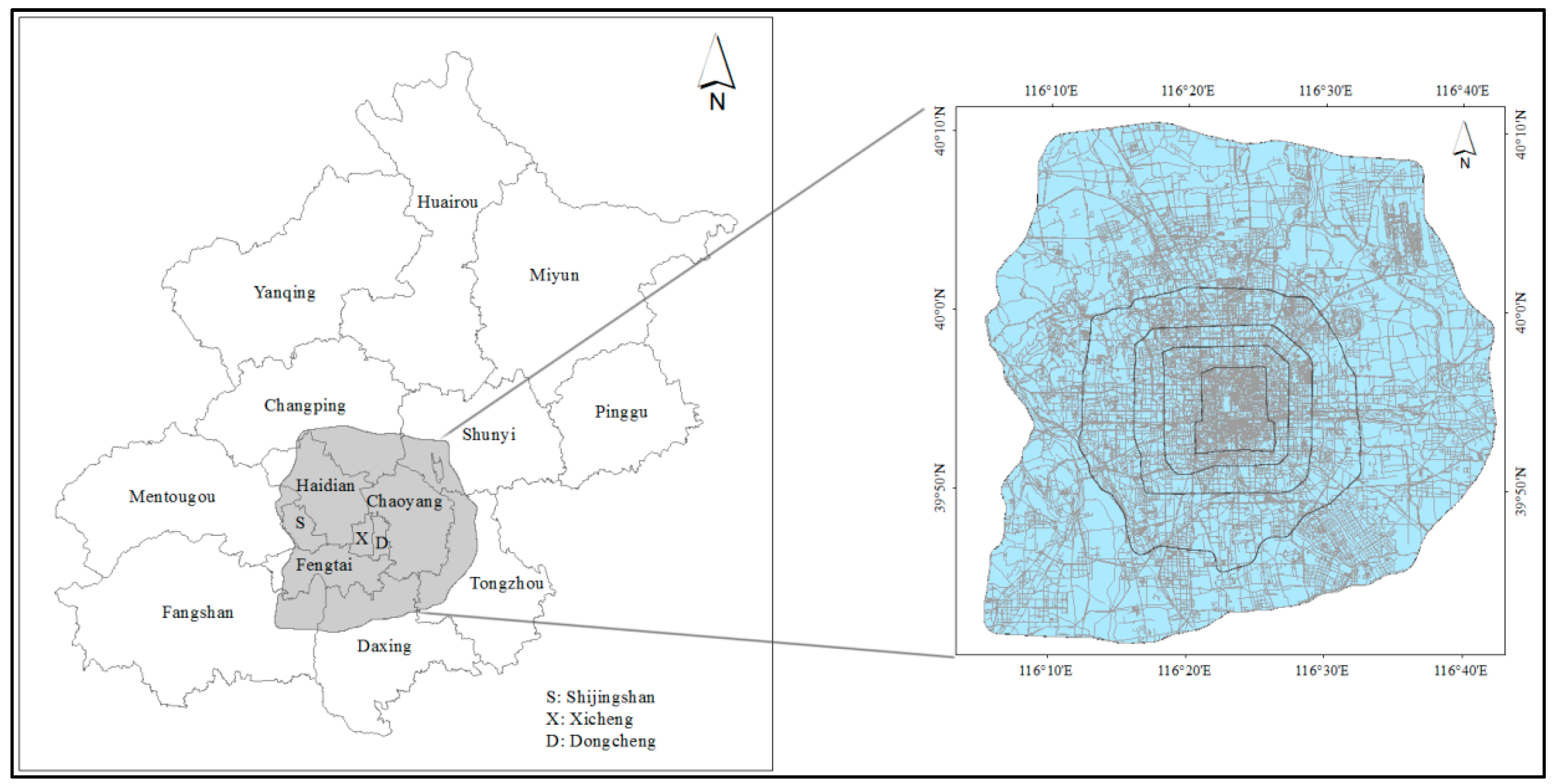
In addition to being the capital of China, Beijing is also the political, economic, and cultural center of China; the city has an area of 12,187 km
2. Its spatial structure is relatively stable. We chose the area within Beijing’s Sixth Ring Road as the study area, which covers 2267 km
2 and accounts for 8% of the total area of Beijing (
Figure 1). As the main urban area of Beijing, it is the core area of economic development in Beijing, comprising many financial institutions, large enterprises, scientific-research institutions, and medical institutions. The area within the Sixth Ring Road in Beijing with a large population has a well-developed street network. Even though the subway is the main mode of public transportation, taxis have been an important component of the urban transportation system in recent years. Taxi data are widely used in analyzing urban functions, urban structures, and human mobility patterns. This research applies a taxi dataset collected from Beijing, China, including more than 15,000 taxis from several anonymous taxi companies in consecutive weeks (6 June to 3 July 2016). The data contain each taxi’s ID, location, sampling time, velocity, and status (vacancy or occupancy of passengers). In this paper, we only extracted the taxi’s ID, the time when the passengers were picked up and dropped off, and the location where the passengers were picked up and dropped off. Usually, the locations of these activities are viewed as the OD of a trip. These extracted trips together reflect the spatial interaction between places.
Table 1 shows an example of the processed taxi data.
POIs collected from Dianping.com were also used in this study to extract the footprint of places. Dianping.com (
http://www.dianping.com/) is an important Chinese e-business platform and independent third-party consumer-review website that was founded in April 2003. Their data are large in terms of volume, and representative. POI refers to all geographic entities that can be abstracted into points. They ignore building areas of solid objects and unify them into areas with no area and no volume, which have the characteristics of a large amount of data, strong real-time performance, and high positional accuracy. We obtained spatial information and attribute the characteristics of shops using POI data, such as the longitude, latitude, name, place, consumption per person, and customer comments. We recorded nearly 80,000 businesses in Beijing on 6 June 2016 with the Application Programming Interface (API) of Dianping.com. Then, we preprocessed these data and retained the following categories: longitude, latitude, name, places. This process not only removes abnormal points, but also removes points that are not within the study area. The data record of a processed POI sample is shown in
Table 2.
2.2. Extracting Place Footprints
Different urban phenomena are always discovered on different study scales. How to select an appropriate spatial-analysis unit is a crucial problem in almost all urban studies. However, there is no clear standard to select one in traditional geographical research [
20]. Improper selection over the course of the study has possibly led to the Modifiable Areal Unit Problems (MAUPs). Some researchers have used regular grids [
21], Voronoi polygons [
22], and roads [
23,
24] as spatial units, which easily cause discontinuities of geographic-property values in a physical space. A place, a polygon, expresses as a geographical area associated with rich semantic features, such as interactions and activities, because it is independent on any scale, and as a reflection of human cognition [
25]. To study vague cognitive places, Li and Goodchild constructed spatial boundaries using kernel-density estimations based on geotagged datasets in Flickr [
26]. Liu et al. proposed a point-set-based region model to approximate vague areal objects and conducted a cognitive experiment to investigate the borders of South China [
27]. Gao et al. assessed the vague cognitive regions of Northern and Southern California by synthesizing multiple heterogeneous datasets from different sources, namely, Flickr, Instagram, Twitter, TravelBlog, and Wikipedia [
28].
Places can provide a new perspective to understanding human cognition and experience in urban environments. Identifying and modeling existing vague places’ footprints in cities are fundamental for urban spatial-structure studies. Dianping.com data offer a new approach to extracting and representing vague places, which is filled in by retailers or customers on the website. The spatial distribution and density of POIs from Dianping.com reflect human cognition of the boundary between these cognitive regions. Extracting the boundaries of vague places is based on fuzzy-set theory [
29], and spatial cognition is commonly used [
27,
30]. Following that theory, we can establish a corresponding membership function like
, and the degree to which an element belongs to a fuzzy set can be expressed by a number between 0 and 1 [
31].
In this research, we applied a three-step workflow to extract continuous boundaries of cognitive places within the Sixth Ring Road of Beijing. In Step 1, we applied the fuzzy-set method based on adaptive kernel-density estimation [
32] for generating scores of each place using POIs. Such scores measure the probability density of the place to which the POI belongs. Higher scores are associated with a higher human recognition of the place, while lower scores represent the opposite. In Step 2, the probability density of each place was converted into the membership degree by the membership function, avoiding the oversimplified representation of continuous surfaces. Such a membership-degree value can be regarded as the possibility of the corresponding position belonging to that place. In Step 3, we constructed polygons from the footprints based on membership-degree contours. Thus, this paper raises some further considerations about multiple vague places. The first one is the overlap between places. Those places can be regarded as geographical borders based on individual spatial cognition. Second, places are not regular divisions of urban spaces, which are the main spaces for people’s activities. Furthermore, cognitive places can also vary in extent, shape, and location among groups and individuals, and can be highly specific to a local population over time; we will not consider this question at this time. In this study, vague regions with a membership degree ≥ 0.5 are known as the generalized cognitive scope of the places. At the same time, if there is an overlapping area that accounts for more than 80% of one place between that place and another, these two places are merged. As a result, we obtained 150 places within the Sixth Ring Road of Beijing, as shown in
Figure 2.
2.3. Construction of Spatial-Interaction Networks
We constructed the SINB with places and their connections. Their nodes are those places extracted before, and the edges are the interplace links connected by taxi trips. The SINB are defined as an undirected weight network . The node set is defined as , where n is the number of nodes. Additionally, the edge set is defined as , where m is the number of edges. To investigate the temporal characteristics of networks, we discretized the taxi data by hourly intervals. All trips extracted from the taxi-trajectory data were aggregated based on the places. The 30-day taxi-trip data were aggregated into one day to generate the 24 OD matrices from the original taxi data. The matrix was set as the one-hour taxi frequency running between nodes. We defined the OD matrix from 0:00 to 1:00 as initial network snapshot , the second one, , was set from 1:01 to 2:00, and the last one, , was set from 23:01 to 24:00.
2.4. Framework Overview
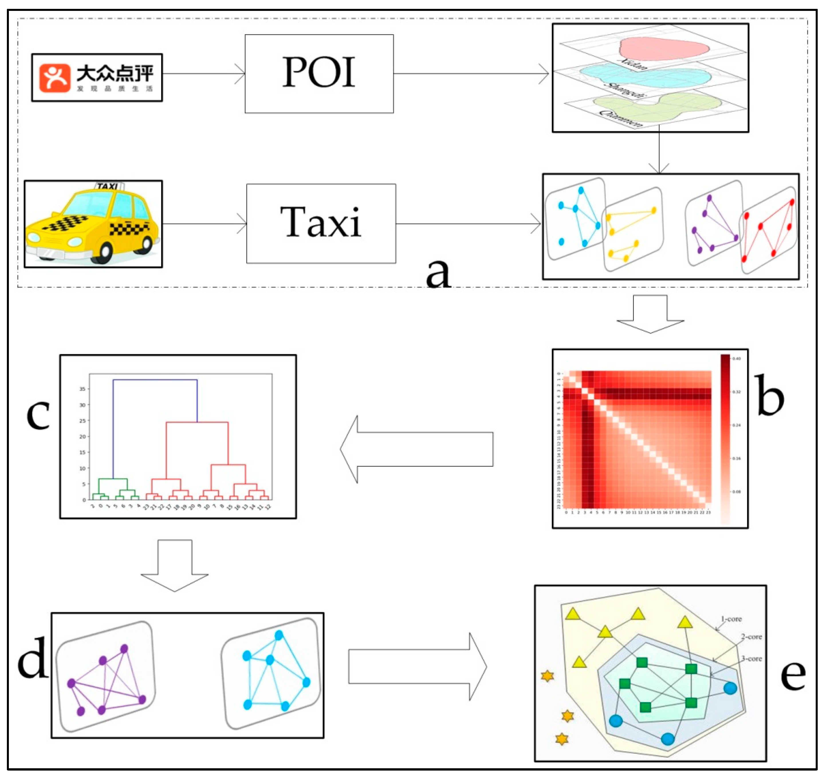
The workflow shown in
Figure 3 is the entire work procedure of analyzing the dynamic characteristics of spatial-interaction networks within the Sixth Ring Road of Beijing in relation to POIs and taxi GPS data. The first part of our work is preprocessing data. The footprints of places and the snapshot networks were extracted from POIs and taxi data, respectively. Then, the distance between each pair of network snapshots was calculated. After that, we ran hierarchical clustering to aggregate the layers when the value of the distance between each pair of layers was smaller than a threshold. Finally, the dynamic hierarchical characteristics of SINB were obtained by the weighted k-core decomposition method.
3. Methods
Many networks change over time. Many traditional network-analysis theories for static networks are also not directly applied to dynamic networks. To explore the SINB evolution process, we transformed sequential temporal snapshots into discrete snapshots. First, we calculated the Jensen–Shannon distance between each pair of network snapshots to quantify the dissimilarity of the 24 layers and obtain the distance matrix between snapshots. Second, we performed classical hierarchical clustering based on the distance matrix to categorize the snapshots into discrete states. Third, the weighted k-core decomposition method was introduced as a tool for studying the spatiotemporal-change network characteristics. Furthermore, some statistical properties of the network structure were used in this paper. Our methods are presented in the following subsections.
3.1. Jensen–Shannon Distance between Snapshots
The present study has not systematically investigated distance measures for networks [
33]. There are many distance measures as the principle or parameter of clustering methods, such as the Graph Edit distance, the DELTACON distance, the Jensen–Shannon distance, the Kullback–Liebler distance, and the Wasserstein distance. In view of our data, the Jensen–Shannon distance measure was experimentally suitable for this research. The Jensen–Shannon distance between two layers was proposed as a dissimilarity measure and cluster layers for networks [
34,
35]. In general, the Jensen–Shannon distance evolved from the Kullback–Liebler distance, and it is more suitable to measure dissimilarity between two matrices. The distance measure based on Jensen-Shannon distance is given by
where
represents Jensen–Shannon distance snapshots i and j, and takes values of [0,1]. The two density matrices
and
correspond to networks
and
, respectively, and
. Neumann entropy is defined by
= −
where
is the i
th eigenvalue of
. Neumann entropy
and
corresponds to matrices
and r, respectively.
3.2. Hierarchical-Clustering Method
The hierarchical-clustering algorithm [
36] is one of the most frequently used methods in unsupervised learning, providing a view of the data at different granularity levels, making it ideal for visualizing and explaining the characteristics of underlying data distribution. The key feature of the traditional method for hierarchical clustering is clustering several variables step by step, and the result of the algorithm is a pyramid structure [
37]. According to the direction of the clustering process, hierarchical methods are divided into agglomerative and divisive [
38]. Hierarchical agglomerative clustering merges the two nearest variables from bottom to top until all variables are merged into an entire variable, while hierarchical divisive clustering is the reverse process. In this paper, the hierarchical-agglomerative-clustering algorithm was applied to process the distance matrix between snapshots. We used the shortest Euclidean distance to define the distance between clusters, and proceeded by repeatedly applying the following three steps:
(1) using the distance between snapshots as variables;
(2) computing the similarity of the pair of variables based on a given distance measure and merging the highest similarity pair into a new cluster; and
(3) updating the similarity between the new cluster and the former existing variables, repeating the procedure until only one node is left.
3.3. Weighted K-Core Decomposition Method
There are various measures applied as an indicator of importance in complex networks, like the centralization index, PageRank, and k-core value. Using the k-core value as an indicator of function is popular. A k-core method is derived by recursively removing all nodes with a degree that is greater than or equal to k until all nodes in the remaining network have a degree of at least k [
39]. A k-core of a graph is any subgraph that has nodes with a degree equal to or larger than k [
40].
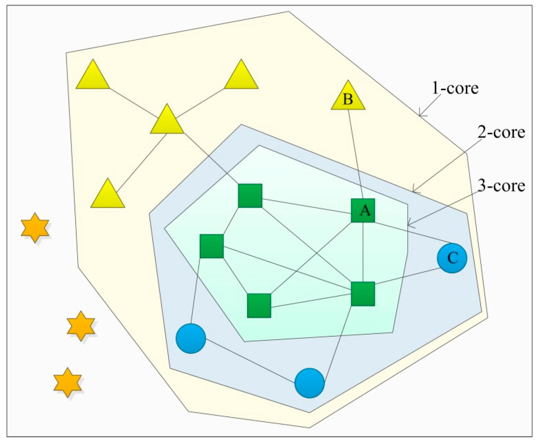
Figure 4 illustrates the decomposition of a given network with 16 nodes. In this implementation, by removing all zero-degree nodes from the network, the remaining nodes from the nodes net are named “one-core”. Then, by recursively deleting all nodes with one degree, the remaining nodes from the nodes’ net are named “two-core”. In a similar manner, the k value is gradually increased and the process is repeated for other nodes until no subgraph exists in the network.
Based on the weighted network decomposition proposed by Caras [
19], this paper redefines the weight of the link considering the spatial weight (distance between nodes) in geographical space. Distance is an important factor affecting spatial interaction that determines the cost of time and interaction. If there are the same spatial interactions and different distances between two nodes, the further the distance is, the more important the connection they have. As shown in
Figure 4, if
=
,
>
, the weight of Link AB is more important than Link AC. Improving the weight of the link based on interaction distance, the new weighted degree of a node i is defined as
where
is the degree of node i;
and
represent the amount and distance of links between origin node i and destination node j, respectively; and
are the adjustment parameters of node degree and node weights. We only considered the case when
in this research. In this implementation, we normalized the entire amount and distance of the links. Similarly, our method is also applicable to directed networks. In addition,
is the sum of the out degree and in degree of node i.
3.4. Additional Methods
The cluster coefficient is usually employed to measure the transitivity of a network. Its value corresponds to the ratio of exiting links to all possible links among the neighbors of a given node. The clustering coefficient of the whole network is the average of all individual clustering coefficients. Average path length is defined as the number of edges along the shortest paths for all possible node pairs in a network. This shows us the average number of steps it takes to get from one member of the network to another. It is a measure of the efficiency of information or mass transport on a network. Usually, a small-world network is identified based on the properties of a high clustering coefficient and low average path length. The diameter of a network is defined as the longest of all the calculated shortest paths.
We move to uncover the tendency of complex connectivity between the three layers of SINB. Here, we define proportion function
as the ratio of connections within the core layer, that is,
where
is the number of links between nodes within the core layer, and n
c is the number of nodes of the core layer. Similarly, the link ratio of the node within the bridge layer and the periphery layer are quantified by
and
, respectively. In addition, we considered the ratio of connections from every layer to its neighbors and defined
as the ratio between the core layer and the bridge layer, which is
where
is the number of links originating from the node in the core layer node to those in the bridge layer, and
is the ratio of links from the core layer to the periphery layer. Furthermore, the ratio of links from the periphery layer to the core layer is quantified by
. Similarly, we defined
,
as the connect ratio between the core layer and the periphery layer, and defined
,
as the connect ratio between the bridge layer and the periphery layer.
4. Results
Previous studies have shown that temporal variations of taxi pick-ups and drop-offs display considerable differences between weekdays and weekends [
41]. Therefore, we separately studied weekdays and weekends in this research. An influential paper about the Internet’s hierarchical structure on the basis of k-core decomposition was published in the Proceedings of the National Academy of Sciences [
39], which merged 42 shells into three layers based on total shell size, largest cluster size, and average distance of the shell. This paper divides SINB nodes into lots of shells, where the coreness of nodes is equivalent in one shell, and then merges the shells into three layers (core layer, bridge layer, and periphery layer) by using natural breaks (Jenks).
4.1. SINB Layer Aggregation
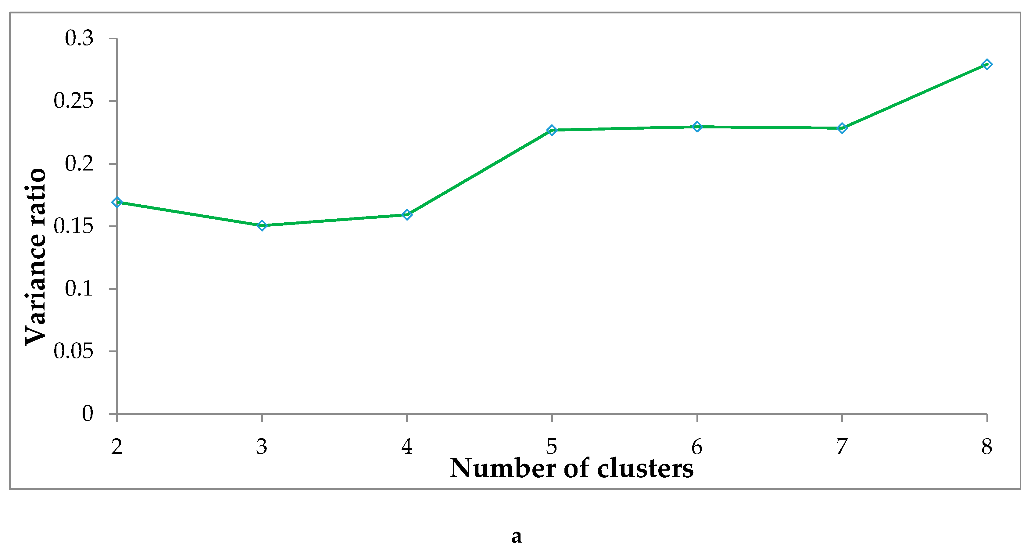
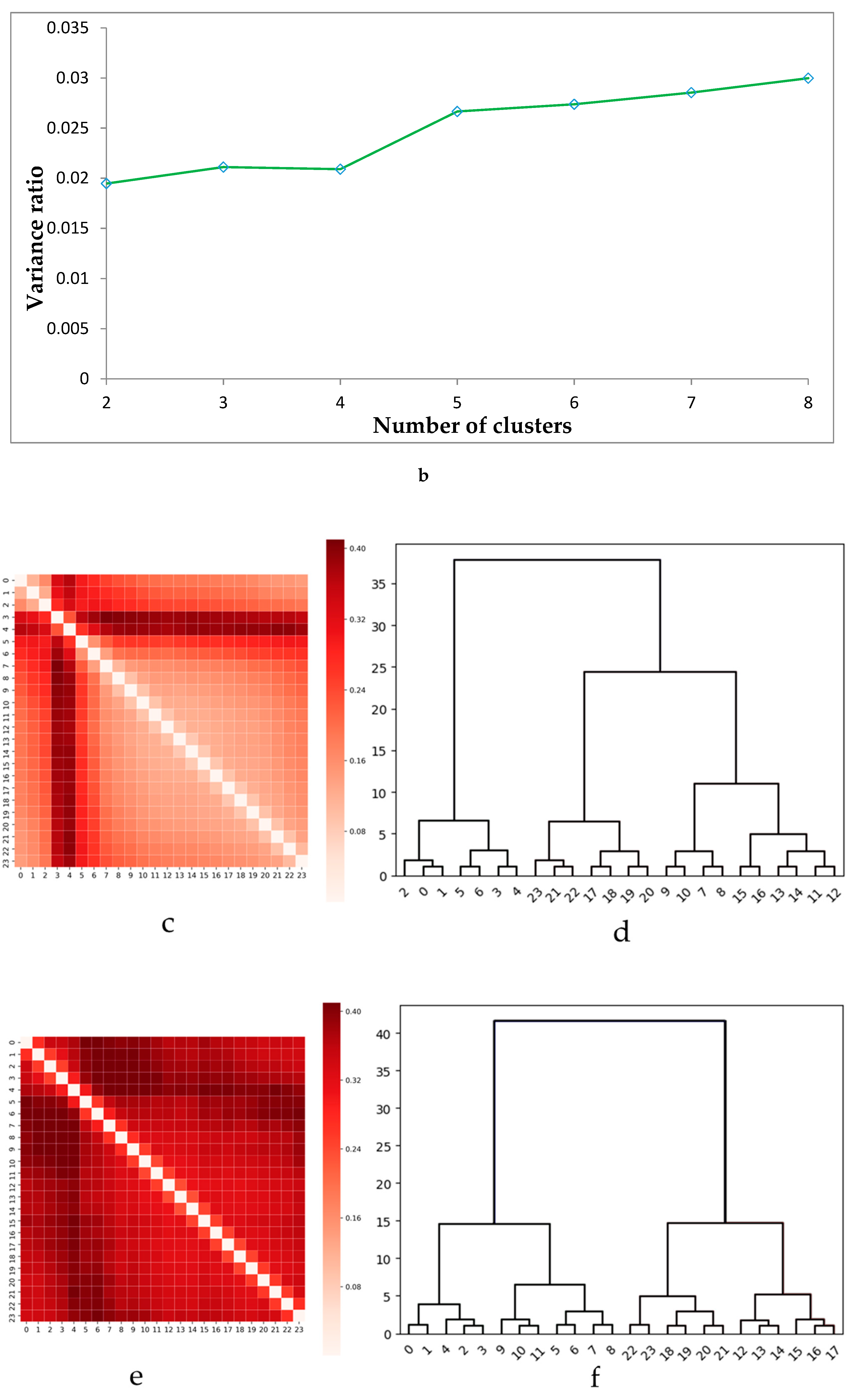
We calculated the ratio of between-cluster variance to the total variance [
42] for each possible k from 2 to 8 to determine the number of clusters k that best divide the data.
Figure 5a illustrates that the variance ratio is small when k = 3 or k = 4 on weekdays. When k = 3, those 24 snapshot networks are marked by three clusters (0–6, 7–16, and 17–23). However, many studies [
4,
43] show that the spatio-temporal change characteristics between 7:00 and 16:00 are flexible and complicated with much more details. Therefore, we selected
on weekdays in our study.
Figure 5b shows that the variance ratio is small when k = 2 or k = 4 on weekdays. Similarly, some details of SINB might be lost when k = 2, and we selected k = 4 on weekends in our study.
The results of the dissimilarity matrix and hierarchical clustering on weekdays are shown in
Figure 5c,d, respectively. The x- and y-axis represent the 24 snapshot networks in
Figure 5c. The heat map represents the dissimilarity between pairs of layers; the darker the color, the higher the dissimilarity. The x-axis represents the 24 snapshot networks, and the y-axis is the interclass distance in
Figure 5d. The result of this procedure is a dendrogram that is a hierarchical diagram where some snapshot networks are the original leaves. At each step of the algorithm, we iteratively aggregated these layers or the clusters of layers with a minimal distance as an internal node. Finally, all original leaves correspond to one root. We obtained a multilayer with fully aggregated graphs. Back to the data, we integrated the 24 snapshot networks into four clusters with different temporal characteristics: early morning (0:00–6:00), morning (7:00–10:00), afternoon (11:00–16:00), and evening (17:00–23:00). For weekends, the heat maps of the dissimilarity matrix and the hierarchical diagram are shown in
Figure 5e,f, respectively. There are some slight differences on the clustering results between weekdays and weekends. The periods of time are early morning (0:00–4:00), morning (5:00–11:00), afternoon (12:00–17:00), and evening (18:00–23:00).
4.2. SINB Change Properties on Weekdays
4.2.1. Properties of Each Layer
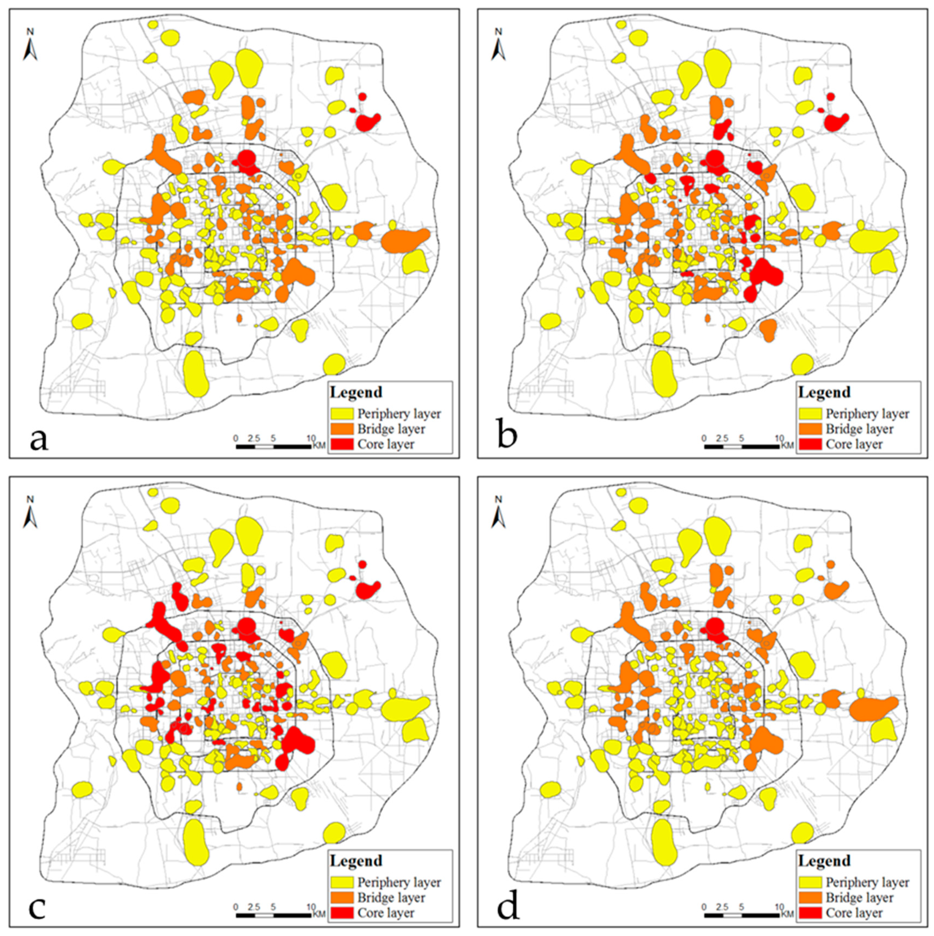
Figure 6 illustrates the distribution of all places we studied in the three layers by order of four periods on weekdays. The important places in the spatial-interaction network exist in the core layer. As a result, the main places are not the same for different periods. Specifically, three main places were extracted: the Asian Games Village–Xiaoying area, Beijing Capital International Airport, and Datun in the early morning. The 14 main places were discovered in the eastern and northern areas of the city, e.g., Beijing Capital International Airport, Datun, the Asian Games Village–Xiaoying area, Zhongguancun, Wangjing, North Taipingzhuang, and Dawang Road in the morning. In the afternoon, the 24 identified main places with a peak level were similar to those places at the last period. A wide distribution occurred in the other three directions between the Third and Fourth Ring, except in the south of the city. The number of main places drops at night. Only two places (Asian Games Village–Xiaoying area and Datun) appeared at this period. The interesting thing is that these two places appear durably in the core layer all day. This is because they have already become a comprehensive downtown area with offices, businesses, residences, and recreational areas since the Olympic Games and Asian Games were held there, respectively. At the same time, some new arrivals, like institutes that have a profound effect on the education industry, led to a strong relation with other places.
The bridge layer connects the core and the periphery as a transition. Places in this layer mainly distribute between the Second and Fifth Ring of the city. There are the same numbers of places in the early morning and in the morning, but different places. The main places include the Summer Palace, Xisi, Chaoyang Park–Tuanjie Lake, Beiyuanjiayuan, and Jinsong–Panjiayuan in the former period, and then move to places like Sijiqing, Wukesong, Jianwai Avenue, Guanzhuang–Changying, and the Yansha Agricultural Exhibition Center. A decreasing trend occurs in the afternoon, during which only 33 places appear, such as Shuangjing, Wudaokou, Xueyuan Bridge, Beiyuanjiayuan, and Zizhu Bridge. However, the number of places increases at night, with a value of 40. Those places, including Beiyuanjiayuan, Beijing Capital International Airport, Jinsong–Panjiayuan, Shibalidian, and Chaoyang Park–Tuanjie Lake, reflect the property of this layer. Some residential districts showed repeated emergence in the four periods, like Zizhu Bridge, Xueyuan Bridge, Wudaokou, Qing River, Shuangjing, Dongzhimen, and Baiziwan.
The peripheral layer is, by definition, the periphery of the network, which is of relatively low importance. Compared to the other two layers, the magnitude of places is greater in order of time period (106, 95, 92, and 108 account for 71%, 63%, 61%, and 72%, respectively). There are constant places responsible for 53% of the total places in the peripheral layer. Their locations are also variously distributed between the Second and the Sixth Ring.
4.2.2. Evolving Topological SINB Characteristics on Weekdays
To further investigate SINB topology properties, we introduced three values: average path length, cluster coefficient, and diameter.
Table 3 illustrates the average path length, cluster coefficient, and diameter of SINB on weekdays. The SINB are similar to a small-world network according to the average path length and cluster coefficient. SINB diameter is the same at the different periods.
In addition, we calculated the value of the top five places with the largest coreness values in the core layer, the bridge layer, and the periphery layer on weekdays, as shown in
Table 4. We found that the cluster coefficient of places increases with the decrement of the coreness of places. This indicates that there is negative correlation between the cluster coefficient and coreness. Places in the core layer tend to connect the places in the bridge and periphery layers, while places in the bridge and the periphery layers have a preference for internal connections.
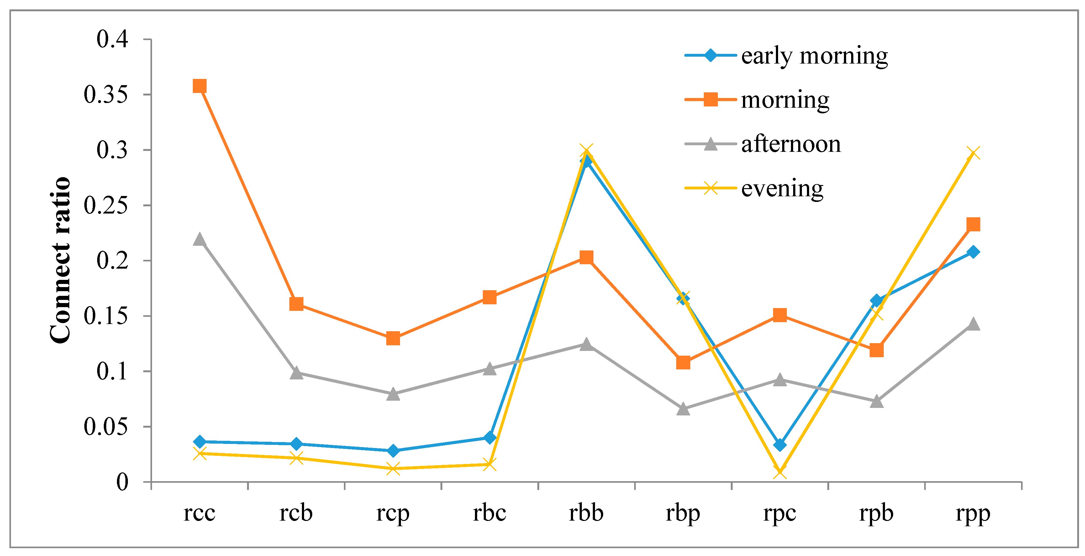
4.2.3. Connection Patterns between Layers and Their Neighbors on Weekdays
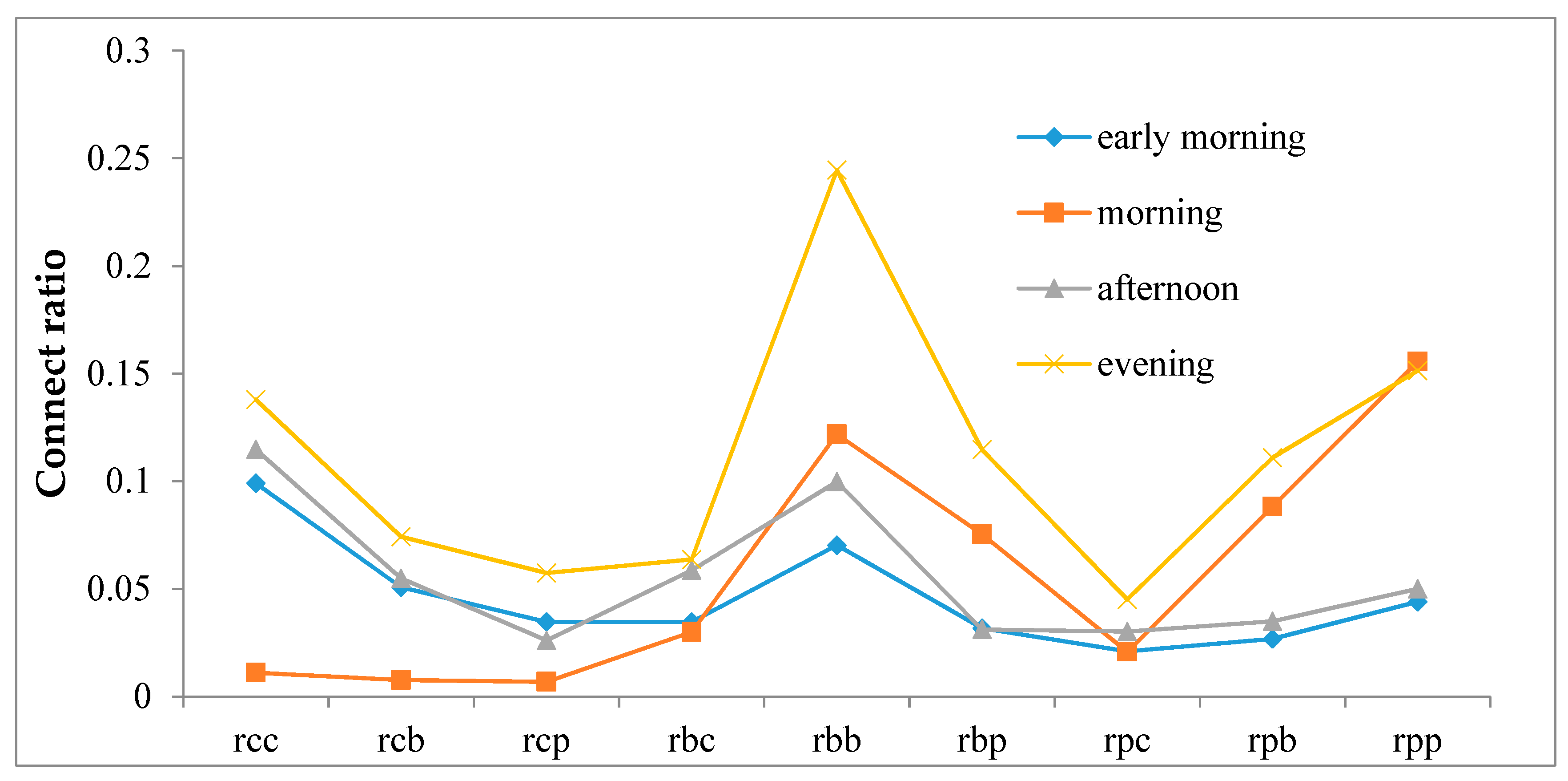
Figure 7 shows the connect ratio of different places in the different layers. Here, the connection patterns are similar in the morning and afternoon. Connections between places that are both in the core layer are stronger than any other types, while places in the bridge layer and in the periphery layer are inclined to connect places in the core layer. Additionally, connection patterns in the early morning and evening are similar, but different from the other two periods. Similarly, there are some inner connections that appeared separately in the bridge and periphery layers.
4.3. SINB Change Properties on Weekends
4.3.1. Properties of Each Layer
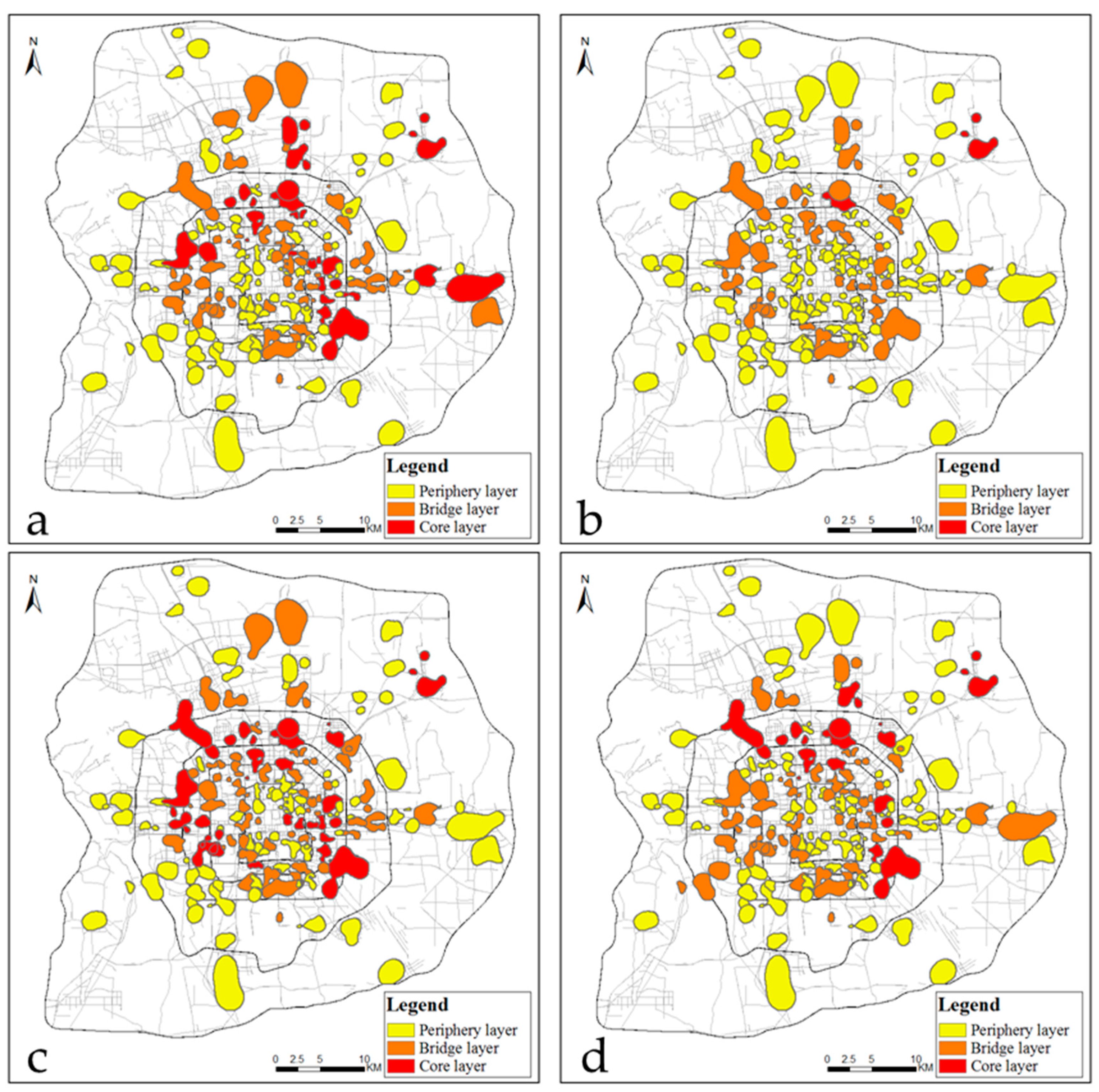
In contrast to the spatial portions of places on weekdays, they remarkably fluctuate in numbers in the core layer as shown in
Figure 8. There are 23 main places located with an interruption of the south of the city in the early morning. Only two places, however, appeared in this layer in the morning: Asian Games Village–Xiaoying and Beijing Capital International Airport. The 23 increasing places spread across the regions between the Second and Fifth Ring Road in the afternoon. In addition, northern and eastern Beijing contributed 15 places, which are all places in this layer that appear at night. Two places (Asian Games Village–Xiaoying and Beijing Capital International Airport) are in core layer at the different periods on weekends.
Most places in the bridge layer are distributed popularly between the Second and the Fifth Ring of the city. The main places were discovered as Jianguomen–Beijing Railway Station, Wangjing, and the Summer Palace (in the early morning); Datun, Shuangjing, and Wangjing (in the morning); Jiuxian Bridge, Sanlitun, and Huangtian Bridge (in the afternoon); and Wukesong, Sijiqing, and Huangtian Bridge (at night). There were also six constant places in this layer, Jiuxian Bridge, Hangtian Bridge, Dewai Avenue, Dahongmen, the Yansha Agricultural Exhibition Center, and Yang Bridge–Muxuyuan.
The number of places in each of the four periods in the peripheral layer is as follows: 84, 114, 76, and 90, comprising 56%, 76%, 51%, and 60% of all places, respectively. There is a large proportion of places in this layer in the morning. This is because residents do not move around on foot too early, and prefer to go on unplanned trips on the weekends. Despite the fact that there is time irregularity in the four periods, 40% of places like Beidadi, Beijing Eastern Railway Station, Caishikou, and Caofang always show up.
4.3.2. Evolving SINB Topological Characteristics on Weekends
As shown in
Table 5, the SINB are also similar to a small-world network on weekends. The lowest clustering coefficient is 0.542549 in the early morning, while the highest is 1.937083 in the evening. Compared with weekdays, the clustering coefficient is lower, the average path length is longer, and the diameter is larger on weekends. It can be seen that humans have most random activities on weekends.
Table 6 shows the value of the top five places with the largest coreness in the core, bridge, and periphery layers on weekends. Similarly, the relationship between the cluster coefficient of places and the decrement of coreness of places has the same trend, and places in the core layer tend to connect places in the bridge and periphery layers, while places in the bridge and periphery layers have a preference for internal connections.
4.3.3. Connections between Nodes and Their Neighbors
Figure 9 illustrates the connection ratio of the core layer, the bridge layer, and the periphery layer on weekends. There are two patterns of connection on weekends that are different on weekdays. There are lots of connections in the bridge and periphery layers and between the bridge layer, and the periphery layer in the morning. The inner-layer connection ratio of each layer is higher, while connections between the layers are relatively low in the afternoon, evening, and early morning.
5. Summary and Discussion
Spatial-interaction networks play a crucial role in the transportation of economics, culture, and the spread of epidemics. Thus, studying and understanding spatial-interaction networks can solve traffic-congestion and urban-planning problems. SINB are also dynamic, which reflects human daily mobility and further reveals the change characteristics of the spatial structure. In this paper, the SINB were studied from the perspective of multilayer temporal networks. First, we used Jensen–Shannon distance and the hierarchical-clustering method to integrate 24 snapshots into four clusters, namely, early morning, morning, afternoon, and evening, and then applied the k-core decomposition method to decompose three layers SINB into four periods to uncover the hierarchical structure, defining three main layers: the core layer, the bridge layer, and the periphery layer. Finally, we analyzed the SINB change characteristics during a day.
We analyzed the SINB on weekdays in order to compare the results between the previous weighted k-core decomposition [
19] method and our method. As
Table 7 shows, the number of different coreness values obtained by the previous weighted k-core decomposition was less than the number found by our method during the same period. This result illustrates that more details of the SINB could be discovered by our method. Specifically, the number of places in the core layer obtained by our method was lower, and those places also appeared in the same layer of previous methods. This means that our method could in some cases identify more important places.
The following conclusions were obtained in this study:
(1) The number was quite different in the each of three layers at the different periods, while spatial distribution stayed relatively stationary. The quantity of places was much smaller in the core layer, and the distribution of places was limited to the area between the Second and Fifth Ring, as well as Beijing Capital International Airport. The number of places in the bridge layer was relatively higher than in the core layer, while their distributions were similar; however, places in the peripheral layer were widely distributed throughout the entire study area.
(2) The SINB stayed compact and connected better, which bears a strong resemblance to a small-world network at the level of topological-feature changes. Moreover, the weekend network had a larger diameter than the weekday one. This reflects that human travel distances on weekends are longer than that on weekdays.
(3) There are two different connection patterns between layers on weekdays and on weekends, respectively. Specifically, on weekdays, the connections of places amass in the core layer from morning to afternoon, while they move to the other two layers during the rest period. On weekends, however, the situation changes. Gathering connections in the peripheral layer in the morning becomes common, and different layers attract internal connections between places in all periods except for in the morning.
Our research offers a new perspective for analyzing urban spatial structures based on the importance of nodes, yet there are limitations to our study. The SINB in the real world are changing over time. Choosing an appropriate time interval could help us to better explore SINB characteristics. As a result, the first problem is our fixed time interval, which might cause significant consequence deviations. In future research, the time span should dynamically change to adapt the temporal features in the network. In addition, the weighted k-core decomposition method that we redefined only considers the distance between nodes, without the direction of the edges. Therefore, the weight of the out- and in-degree in k-core decomposition should be considered.


