Eigenvector Spatial Filtering-Based Logistic Regression for Landslide Susceptibility Assessment

Abstract

Logistic regression methods have been widely used for landslide research. However, previous studies have seldom paid attention to the frequent occurrence of spatial autocorrelated residuals in regression models, which indicate a model misspecification problem and unreliable results. This study accounts for spatial autocorrelation by implementing eigenvector spatial filtering (ESF) into logistic regression for landslide susceptibility assessment. Based on a landslide inventory map and 11 landslide predisposing factors, we developed the eigenvector spatial filtering-based logistic regression (ESFLR) model, as well as a conventional logistic regression (LR) model and an autologistic regression (ALR) model for comparison. The three models were evaluated and compared in terms of their prediction capability and model fit. The ESFLR model performed better than the other two models. The overall predictive accuracy of the ESFLR model was 90.53%, followed by the ALR model (76.21%) and the LR model (74.76%), and the areas under the ROC curves for the ESFLR, ALR and LR models were 0.957, 0.828 and 0.818, respectively. The ESFLR model adequately addressed the spatial autocorrelation of residuals by reducing the Moran’s I value of the residuals to 0.0270. In conclusion, the ESFLR model is an effective and flexible method for landslide analysis.

1. Introduction

Landslides are the most common natural geological disasters and cause damage to infrastructure and natural ecology, resulting in serious casualties and economic losses [1]. Therefore, research on landslides has become an urgent task to reduce their detrimental impacts.

For decades, landslide research has been a popular topic among the research communities. Many different methods have been utilized to reveal the link between landslide occurrence and various controlling factors for the purpose of landslide prediction, such as logistic regression [2,3,4], the information value method [5,6,7], frequency ratio [8], analytic hierarchy process [9,10], artificial neural network [11,12] and support vector machine [13]. Among the various methods, the logistic regression (LR) method has been widely used and reported to be applicable for landslide research [14,15,16,17]. Logistic regression provides a significant advantage in that, with an appropriate link function, the variables can be continuous, discrete or a combination of the two types, without necessarily having a normal distribution [15].

However, Tobler’s first law of geography [18] indicates that spatial data are not independent but geographically relevant within a given geographic surface area—this is called spatial autocorrelation. Spatial autocorrelation [19] is commonly observed in spatial data, and regression models applied to these data often contain spatially autocorrelated residuals. However, previous landslide studies using logistic regression for landslide prediction rarely took spatial autocorrelation into account [20], which implies that these models failed to explain all of the spatial patterns inherent in the landslide data, and may have led to misspecification errors in the model.

This study attempted to eliminate the negative influence of spatial autocorrelation on landslide susceptibility assessments by introducing eigenvector spatial filtering (ESF) into logistic regression. Spatial filtering, as discussed by Getis [21,22] and Griffith [23], was considered to be an effective approach for addressing spatial autocorrelation. The ESF method proposed by Griffith, utilizes eigenvectors generated from a given spatial connectivity matrix to account for redundant locational information resulting from spatial autocorrelation [24]. Several significant eigenvectors selected with a stepwise regression procedure are added to the linear regression model as independent variables to filter the spatial autocorrelation out from the regression residuals.

This study was conducted in Wulong county and involved four main steps. First, the predisposing factors responsible for landslide occurrence were determined. Subsequently, landslide susceptibility models were developed. Then, evaluations were conducted and comparisons were made between the ESF-based logistic regression model and other models, including ordinary logistic regression and autologistic regression, to assess model performance. Finally, the models were employed to map landslide susceptibility throughout the study area.

2. Study Area and Data

2.1. Study Area

The study area of Wulong county is located in the southeast section of the Chongqing Municipality (Figure 1) between longitudes (107°14′) E and (108°5′) E and latitudes (29°2′) N and (29°40′) N, and covers an area of approximately 2900 km². The Wujiang River travels through the whole territory from east to west with a total distance of 80 km, running through 16 towns. The geological structure of the Wulong area was formed in the second stage of the Yanshanian period, which belongs to the Neocathaysian tectonic system and the north-south radial tectonic system. Wulong county is a mountainous area with many deep valleys and steep hills, and the terrain is high in the northeast and low in the southwest. The area belongs to the South China Karst. During the geological process, severe dissolution formed a complex landform with many interlaced deep trough valleys. The study area has a typical subtropical monsoon climate, with annual rainfall generally more than 1000 mm and a rainy season normally concentrated in summer. The annual average temperature is between 15 °C and 18 °C. The Wulong area is prone to landslides due to its peculiar terrain, and its stratum, which mostly consists of unstable rock masses with severe weathering conditions.

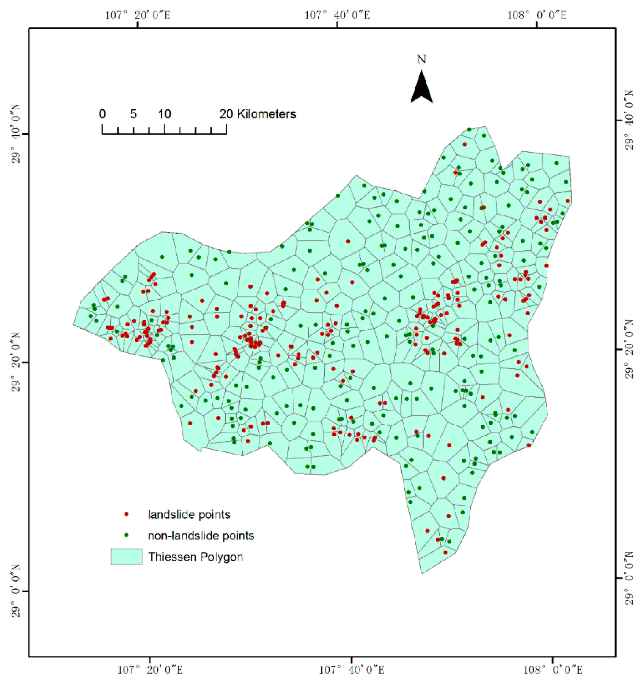
2.2. Landslide Inventory Map

In this study, a total of 206 landslides that were documented by the Chongqing Institute of Geology and Mineral Resources by 2014 are represented in the form of point features in the landslide inventory map (Figure 1). Unfortunately, the information on landslide type in the study area was not recorded due to irregularities in the data collection process. Each landslide point has its own attributes, including latitude and longitude and covered area. The 206 landslides covered a total area of 6,367,050 m² with an average of 30,908 m², of which the largest landslide was 500,000 m² and the smallest was 600 m². We divided the landslides into small-sized (<50,000 m²), medium-sized (50,000~100,000 m²) and large-sized (≥100,000 m²) landslides according to their area of coverage. Small-sized landslides accounted for approximately 84.47% of the total landslides, approximately 12.62% of landslides were medium-sized, and only 6 of the 206 landslides were larger than 100,000 m². As can be observed in the inventory map, most of the landslide points are distributed along the hydrological network, road network and fault lines.

2.3. Landslide Predisposing Factors

The occurrence of landslides is triggered by a combination of many internal and external factors. It is well known that there are no general criteria for factor selection [25]. The key factors that trigger landslides mainly include topographic and geological factors, hydrological and climatic conditions, vegetation coverage and human engineering activities [26]. In this paper, considering the complex conditions in Wulong county and taking data availability into account, 11 factors, including elevation, slope, aspect, curvature, distance to road, distance to railway, distance to river, distance to fault, precipitation, lithology and NDVI (normalized difference vegetation index), were identified as landslide predisposing factors for landslide analysis.

Topographic factors have strong controlling effects on landslides. Wulong county is prone to landslides due to its complex landform, steep slopes and large elevational differences. Therefore, important topographic factors such as elevation, slope, aspect and curvature were considered landslide predisposing factors. Elevation is a frequently used factor for landslide analysis because of its strong relationship with landslides. Landslides are more likely to occur in moderately elevated areas where the slopes are often covered by thin colluvium [27]. Slope is generally considered an important factor affecting landslides. On a uniform and isotropic slope, in theory, the likelihood of slope failure increases with the increase in slope. However, Eeckhaut et al. [28] noted that landslides are actually more prone to occur over moderate slopes. The distributions of soil, water, and vegetation vary with different slope aspects, which leads to different slope stabilities [29]. The curvature data used in this paper represent the general curvature, which can help to characterize slope morphology and flow [30]. The digital elevation model (DEM) for Wulong county was derived from geospatial data cloud (GS Cloud) with a resolution of 30 m × 30 m. Elevation, slope, aspect and curvature were extracted based on the DEM. The elevation map, slope map, aspect map, and curvature map are shown in Figure 2. Human activities, especially the construction of infrastructures can destroy the stability of a slope and result in increased landslide risk. The road and railway data obtained from OSM (Open Street Map) were applied to map the distance to the road (Figure 2e) and the distance to the railway (Figure 2f), respectively. The distance to a river is associated with landslide occurrence due to water erosion, and the distance to a river map (Figure 2g) was generated using the hydrological network data from OSM. The areas in the vicinity of a fault have a higher incidence of landslides; hence, the distance to a fault was considered a significant factor. The fault data for the Wulong area, which was generated from the Chongqing construction outline map at a scale of 1:500,000 through geography registration and digitization, was used to produce a map for the distance to a fault (Figure 2h). Rainfall makes an important contribution to the development of landslide disasters, and it has been indicated that landslides occur more often with continuous heavy rain. Through a literature search, Budimir et al. [4] indicated that rainfall could be considered both a conditioning factor (long-term) and a triggering factor (short-term). Annual precipitation, which reflects regional rainfall intensity and duration in the long term, is a conditioning factor that is frequently used for landslide research. Areas with more annual rainfall are more prone to landslides. The Chongqing Institute of Geology and Mineral Resources also provided the daily rainfall data from 1003 rainfall observation stations for the period from 2005–2014. The mean annual precipitation at 78 rainfall observation stations within and near the Wulong area was calculated and used to create the precipitation map (Figure 2i) for the whole study area by using the inverse distance interpolation method. Different lithologies have various effects on landslide development. The lithology map (Figure 2j) was generated using the geological map of Sichuan and Chongqing at a scale of 1:2,500,000. Vegetation cover can help consolidate mountains and reduce erosion by rainfall, thus effectively reducing the landslide risk. Therefore, the NDVI, which measures vegetation coverage, was included in this study. The NDVI map (Figure 2k) was obtained by calculation according to the formula NDVI = (IR − R)/(IR + R), where IR and R are the near-infrared and red bands of Landsat 8 OLI_TRIS satellite images, respectively.

3. Methods

3.1. Generation of Landslide Dataset

Landslide prediction based on the logistic method is actually a binary classification process, in which the landslide probability, which varies from 0 to 1, is divided into two categories: presence and absence of landslides. Therefore, for the purpose of constructing models, it is necessary to build a spatial landslide dataset, including landslide points and non-landslide points. We designated the landslide points as 1 whereas the non-landslide points are designated as 0. The selection of non-landslide points is crucial since it determines whether the samples represent the overall characteristics of the study area.

Thus, the following two principles should be observed during the selection of non-landslide points: (1) non-landslide points should maintain a certain distance from historical landslide areas; and (2) non-landslide points should be distributed as evenly as possible to avoid the cluster effect, which may cause model error.

We designed the selection method, and the details are as follows: the landslide-affected area can be determined with each landslide point as the center and the corresponding landslide-affected distance as the radius to derive the buffer zones. The landslide-affected distance, namely, the multiple of the landslide radius, can be derived as shown in Equation (1).

$$D=\rho \sqrt{\frac{A}{\pi }}$$

(1)

where D denotes the landslide-affected distance, A denotes the landslide area, $\rho$ denotes a proportionality constant, which is 1000 in this study.

The landslide-free area, in which the non-landslide points are randomly generated, is obtained by removing the landslide-affected area from the study area. The number of newly generated non-landslide points is identical to the number of landslide points, and both are combined to form the landslide dataset.

As mentioned in the previous section, 11 factors that have inducing effects on landslide occurrence were prepared for landslide susceptibility modeling. Aspect is generally divided into nine categories: flat, north, northeast, east, southeast, south, southwest, west and northwest (Figure 2c), and the lithology of the study area also has nine categories: slate, basalt, limestone, glimmerite, marlite, sandstone, clastic rock, phyllite and mudstone (Figure 2j). Therefore, to ensure the correspondence of the factors, all 11 landslide predisposing factors are classified into 9 classes. In this paper, 9 other continuous factors were classified using the natural breaks (Jenks) method to minimize the squared deviation within each class and maximize the difference between classes. Considering the different dimensions and value ranges of each factor, we used the frequency ratio (R value) to unify the dimensions of each factor. The R value of class i of a factor was defined as:

$$R_i=\frac{A_i/A}{S_i/S}$$

(2)

where $A_i$ is the landslide area that fell into class i, $S_i$ is the area covered by the same class, A is the total landslide area in the study area, and S is the total area of the study area. The R value was calculated for each class of the 11 factors (

Table 1. The R values for the classes of the landslide predisposing factors.

Factors	Class	Landslide Area (Ai)	Landslide Area Ratio (Ai/A)	Class Area Ratio (Si/S)	Frequency Ratio (R)
Elevation	1	141.28	0.22	0.09	2.6
	2	172.36	0.27	0.11	2.52
	3	90.14	0.14	0.13	1.12
	4	121.63	0.19	0.14	1.37
	5	34.78	0.05	0.14	0.4
	6	75.56	0.12	0.13	0.91
	7	0.96	0	0.12	0.01
	8	0	0	0.08	0
	9	0	0	0.07	0
Slope	1	37.99	0.06	0.11	0.54
	2	213.74	0.34	0.16	2.08
	3	148.79	0.23	0.18	1.29
	4	102.71	0.16	0.17	0.96
	5	56.79	0.09	0.14	0.64
	6	39.98	0.06	0.11	0.6
	7	28.02	0.04	0.07	0.6
	8	4.66	0.01	0.04	0.17
	9	4.03	0.01	0.02	0.37
Aspect	1	0	0	0	0
	2	42.65	0.07	0.1	0.64
	3	96.65	0.15	0.12	1.27
	4	122.45	0.19	0.15	1.31
	5	73.95	0.12	0.15	0.76
	6	79.07	0.12	0.1	1.18
	7	69.47	0.11	0.11	0.98
	8	58.72	0.09	0.13	0.71
	9	93.75	0.15	0.13	1.13
Curvature	1	0	0	0	0
	2	1.75	0	0.02	0.16
	3	46.02	0.07	0.07	1.04
	4	174.59	0.27	0.21	1.29
	5	303.37	0.48	0.4	1.19
	6	79.75	0.13	0.21	0.61
	7	28.06	0.04	0.07	0.62
	8	2.47	0	0.02	0.21
	9	0.7	0	0	0.45
Distance to Road	1	303.55	0.48	0.28	1.71
	2	145.05	0.23	0.24	0.95
	3	75.04	0.12	0.18	0.66
	4	87.33	0.14	0.12	1.1
	5	16.4	0.03	0.08	0.32
	6	1.34	0	0.05	0.04
	7	2.7	0	0.02	0.17
	8	0.5	0	0.01	0.06
	9	4.8	0.01	0.01	0.81
Distance to Railway	1	122.16	0.19	0.17	1.11
	2	193.82	0.3	0.18	1.7
	3	139.24	0.22	0.16	1.4
	4	102.95	0.16	0.14	1.16
	5	39.85	0.06	0.11	0.55
	6	19.87	0.03	0.09	0.34
	7	11.73	0.02	0.07	0.25
	8	0.45	0	0.05	0.01
	9	6.64	0.01	0.03	0.37
Distance to River	1	260.26	0.41	0.25	1.65
	2	107.62	0.17	0.22	0.76
	3	148.41	0.23	0.18	1.27
	4	41.76	0.07	0.12	0.54
	5	57.58	0.09	0.08	1.12
	6	8.26	0.01	0.06	0.22
	7	10.68	0.02	0.04	0.46
	8	1.24	0	0.03	0.06
	9	0.9	0	0.02	0.08
Distance to Fault	1	44.5	0.07	0.16	0.44
	2	42.93	0.07	0.17	0.4
	3	66.51	0.1	0.15	0.71
	4	142.69	0.22	0.13	1.78
	5	144.28	0.23	0.11	2.05
	6	68.69	0.11	0.1	1.06
	7	63.92	0.1	0.09	1.15
	8	58.06	0.09	0.07	1.38
	9	5.13	0.01	0.04	0.23
Precipitation	1	7.88	0.01	0.02	0.63
	2	7.01	0.01	0.06	0.18
	3	18.02	0.03	0.14	0.2
	4	92.97	0.15	0.14	1.03
	5	92.69	0.15	0.17	0.88
	6	239.65	0.38	0.17	2.16
	7	114.66	0.18	0.18	1
	8	57.63	0.09	0.1	0.89
	9	6.2	0.01	0.02	0.54
Lithology	1	98.33	0.15	0.48	0.32
	2	131.2	0.21	0.16	1.31
	3	7.45	0.01	0	3.95
	4	2.14	0	0	1.76
	5	6.18	0.01	0	7.36
	6	195.11	0.31	0.2	1.57
	7	36.02	0.06	0.01	4.78
	8	11.5	0.02	0	7.95
	9	148.78	0.23	0.14	1.63
NDVI	1	15.8	0.02	0.06	0.41
	2	32.84	0.05	0.08	0.68
	3	77.74	0.12	0.09	1.29
	4	63.21	0.1	0.12	0.81
	5	127.43	0.2	0.14	1.45
	6	123.43	0.19	0.15	1.26
	7	135.46	0.21	0.15	1.38
	8	57.2	0.09	0.13	0.69
	9	3.6	0.01	0.07	0.08

R: frequency ratio, as defined in Equation (2).

) and was extracted for both the landslide points and the non-landslide points for subsequent model construction as the independent variables. The R value takes the prior knowledge of landslides into account, and the class with higher R values is more prone to landslides in the case. It should be noted that since only landslide point data are available in this study, when a landslide point falls in class i, it is considered that the landslide area falls completely in class i, regardless of whether a landslide may cover more than one class.

3.2. Multicollinearity Analysis

Collinearities among independent variables may result in distortion in the model’s estimation [31]. Multicollinearity diagnosis was conducted using tolerance (TOL) and the variance inflation factor (VIF) [32]. VIF can be calculated using the vif function housed in the “car” R package. TOL is actually the reciprocal of VIF, namely, TOL = 1/VIF. Both TOL values close to 0, and large VIF values indicate serious multicollinearity. Only independent variables with VIF values over 2 and TOL values less than 0.4 are be excluded from the regression modeling [33]. In this paper, the two indexes for each factor were calculated, and the results suggested that the multicollinearity was weak among the 11 landslide predisposing factors; thus, no factor needed to be excluded (

Table 2. Multicollinearity analysis for the landslide predisposing factors.

Landslide Predisposing Factor	TOL	VIF
Elevation	0.827	1.209
Slope	0.97	1.031
Aspect	0.982	1.019
Curvature	0.966	1.036
Distance to Road	0.795	1.258
Distance to Railway	0.804	1.244
Distance to River	0.779	1.284
Distance to Fault	0.93	1.075
Precipitation	0.895	1.117
Lithology	0.952	1.05
NDVI	0.966	1.035

).

3.3. Eigenvector Spatial Filtering Based on Logistic Regression Modeling

Spatial data always have a certain degree of spatial autocorrelation. Eigenvector spatial filtering is a relatively new approach that aims to filter the spatial autocorrelation out of the regression residuals to obtain a modified and enhanced model. The model contains a linear combination of appropriate eigenvectors, which were extracted from the spatial connectivity matrix C, as additional independent variables of the regression model.

Landslide susceptibility modeling using eigenvector spatial filtering-based logistic regression (ESFLR) involves four main steps as follows:

(1) Construction of the spatial connectivity matrix C of the landslide point dataset, including 206 landslide points and 206 non-landslide points. Either topology-based or distance-based methods can be used to construct the spatial connectivity matrix [34]. In this paper, we constructed Thiessen polygons of 412 discrete observation points with ArcGIS software (Figure 3) to determine the spatial neighbor relationship of the polygon features rather than the point features. A binary topology-based matrix C was considered more appropriate here and was established from the Thiessen polygons. Thus, based on the landslide dataset derived in Section 3.1, we obtained an n-by-n matrix (n = 412 in this study), and if polygon i and polygon j were neighbors, $c_{ij}=1 \left(1\le i\le 412, 1\le j\le 412\right)$, otherwise $c_{ij}=0$.

(2) Computation of eigenvectors and associated eigenvalues. The computation is based on a mathematical decomposition of the following matrix MCM transformed by the projection matrix M =$\left(I-\frac{{11}^T}{n}\right)$:

$$\mathrm{MCM}=\left(I-\frac{{11}^T}{n}\right)C\left(I-\frac{{11}^T}{n}\right)$$

(3)

where $I$ is an n-by-n identity matrix, $1$ is an n-by-1 vector whose elements are all 1, and $T$ is the matrix transpose operator. The decomposition can be expressed as:

$$\mathrm{MCM}=E\Lambda E^T$$

(4)

The decomposition of MCM generates eigenfunctions that contain n eigenvectors and n corresponding eigenvalues [35]. The n eigenvectors can be denoted as $E=\left(E_1,E_2,\cdots ,E_n\right)$, and each eigenvector is capable of capturing latent spatial autocorrelation at different scales [36]. $\Lambda$ is an n-by-n diagonal matrix, and its diagonal elements are the n eigenvalues, which can be denoted in descending order as $\lambda =\left({\lambda }_1,{\lambda }_2,\cdots ,{\lambda }_n\right)$. Therefore, the first eigenvector, $E_1$, has the largest eigenvalue ${\lambda }_1$, and the last eigenvector, $E_n$, has the smallest eigenvalue ${\lambda }_n$. It should be noted that all eigenvectors are orthogonal, and all eigenvector pairs are uncorrelated to each other [23].

(3) Stepwise selection of eigenvectors. The eigenvectors that can reduce the spatial autocorrelation of residuals to the maximum extent are added to the model. Since the response variable in this study exhibits a significant positive spatial autocorrelation with a Moran’s I value of 0.616, the eigenvectors with negative Moran’s I values are first removed. The eigenvectors with larger positive Moran’s I values that are considered, in theory, to be able to explain or filter out more spatial autocorrelation from the regression residuals are regarded as candidate eigenvectors. There is a function relationship between Moran’s I value of the ith eigenvector (E_i) and its corresponding eigenvalue (${\lambda }_i$), which can be expressed as:

$$M{I}_i=\frac{n}{1^{T}C1}{\lambda }_i$$

(5)

The criterion generally used for identifying the candidate subset is a Moran’s I value greater than 0.25 [35].

Then, a stepwise regression selection approach is implemented to identify the final eigenvectors from the candidate subset to be included in the logistic model. In this approach, the eigenvectors are selected iteratively. For each iteration, the eigenvector that minimizes the spatial autocorrelation of residuals is selected. Each eigenvector in the candidate subset was added as an additional independent variable into the logistic model one by one to fit the model, and the Moran’s I values of the model residuals were calculated. The corresponding eigenvector with the smallest Moran’s I value was considered to be added into the final model and removed from the candidate subset. A permutation test was conducted for each newly added eigenvector to test the significance of the spatial autocorrelation of regression residuals, which is commonly measured by Moran’s I. The selection procedure continued until Moran’s I was no longer significant.

(4) ESFLR modeling. A linear combination of the selected eigenvectors was incorporated into the logistic regression as additional explanatory variables to account for latent spatial autocorrelation. Regarding landslide susceptibility modeling, logistic regression (LR) is expected to reveal the contribution of a series of landslide predisposing factors. The LR model can be expressed as:

$$Y=logit\left(P\right)=\ln \left(\frac{P}{1-P}\right)={\beta }_0+{\beta }_1{X}_1+{\beta }_2{X}_2+\cdots +{\beta }_n{X}_n$$

(6)

where P denotes the probability of landslide occurrence,${\beta }_0$ denotes the intercept and ${\beta }_i\left(i=1,2,\cdots ,n\right)$ are the regression coefficients of the independent variables ($X_i\left(i=1,2,\cdots ,n\right)$). The ESFLR, analogously, can be written as follows:

$$Y={\beta }_0+{\beta }_1{X}_1+{\beta }_2{X}_2+\cdots +{\beta }_n{X}_n+{\beta }_k{E}_k+\epsilon$$

(7)

where E_k is a matrix containing the k selected eigenvectors, ${\beta }_k$ is a vector containing the associated regression coefficients, and $\epsilon$ is an error vector. The ESFLR does not suffer from spatial autocorrelation among residuals since ${\beta }_k{E}_k$ accounts for this spatial autocorrelation. For the sake of landslide susceptibility, the landslide probability P can be calculated by the following transformed formula:

$$P=\frac{1}{1+e^{-Y}}$$

(8)

3.4. Model Validation

To verify the performance of the ESFLR model, the ESFLR model and other alternative models, including the ordinary logistic regression (LR) and the autologistic regression (ALR), were evaluated and compared. The LR model has been introduced in Section 3.3. Autologistic regression addresses spatial autocorrelation by adding an autocovariate as a further explanatory variable in logistic regression [37]. The autocovariate is calculated for each cell as the weighted (usually inverse distance) average of the landslide susceptibility values of its neighbors [38,39].

$$Autoco{v}_i=\frac{{{\displaystyle \sum }}_{j=1}^{k_i}{w}_{ij}{p}_j}{{{\displaystyle \sum }}_{j=1}^{k_i}{w}_{ij}}$$

(9)

where $p_j$ is the response value, i.e., landslide susceptibility, of cell j among $k_i$ neighbors of cell I, which is derived from the LR model, and $w_{ij}$ is the weight defined as the inverse Euclidean distance between cell i and j. The logistic regression model can be transformed into an autologistic model as follows:

$$Y={\beta }_0++{\beta }_1{x}_1+{\beta }_2{x}_2+\cdots +{\beta }_n{x}_n+rAutoco{v}_i$$

(10)

where r is the estimated coefficient of $Autoco{v}_i$.

The above three models were validated and compared with each other in terms of the following three aspects.

(1) Model performance. In this paper, the model performance was assessed in terms of the model prediction capability and model fit using statistical measures and the ROC curve. To assess the classification ability of the model on both landslide and non-landslide points, three parameters calculated from the confusion matrixes were applied including overall accuracy, positive accuracy, and negative accuracy [40].

$$\mathrm{Overall}\mathrm{accuracy}=\frac{\mathrm{TP}+\mathrm{TN}}{\mathrm{TP}+\mathrm{TN}+\mathrm{FP}+\mathrm{FN}}$$

(11)

$$\mathrm{Positive}\mathrm{accuracy}=\frac{\mathrm{TP}}{\mathrm{TP}+\mathrm{FP}}$$

(12)

$$\mathrm{Negative}\mathrm{accuracy}=\frac{\mathrm{TN}}{\mathrm{TN}+\mathrm{FN}}$$

(13)

where TP (true positive) is the number of landslide points correctly classified into class 1 (presence of landslide), FP (false positive) is the number of landslide points wrongly classified into class 0 (absence of landslide), TN (true negative) is the number of correctly predicted non-landslide points, and FN (false negative) is the number of incorrectly predicted non-landslide points. The landslide probability values derived from the three models fall between 0 and 1, with higher values indicating higher landslide risk. In this study, 0.5 was selected as the threshold, and points with landslide probability values greater than 0.5 were classified as class 1; otherwise, the points were classified as class 0.

The ROC curve (receiver operating characteristics curve) is a useful and widely implemented method for evaluating model performance [41,42]. The performance of a model can be evaluated quantitatively using the AUC (area under the curve) value, which ranges from 0 to 1. It is generally believed that the greater the AUC value is, the better the model will perform. The model exhibits certain accuracy when the AUC value is between 0.7 and 0.9, and it indicates high accuracy if the AUC value of a model is greater than or equal to 0.9.

Furthermore, the Nagelkerke R² and AIC (Akaike information criterion) values were also considered as model evaluation measures. The Nagelkerke R² is a kind of pseudo R² similar to R² in linear regression [43], which can serve as a measure of the goodness of fit of a logistic regression model. The Nagelkerke R² value falls between 0 and 1, with higher values suggesting better model fit. The AIC value considers model fit as well as model complexity. A smaller AIC value indicates that the model achieves higher goodness of fit with fewer variables.

(2) Ability to eliminate spatial autocorrelation of residuals. Moran’s I is the most common quantitative measure of spatial autocorrelation in regression residuals [44]. In our study, spatial autocorrelation in regression residuals was detected using global Moran’s I to verify the effectiveness of the models in addressing spatial autocorrelation.

(3) Generalization capacity. K-fold cross validation (CV) with k = 10 in this study was performed to test the generalization capacity of the models [45]. First, the landslide dataset is divided into k equal sub-datasets at random. Among the k sub-datasets, each individual sub-dataset will serve as the validation data for validating the model fitted by the remaining k − 1 sub-datasets [46]. The CV process is repeated k times, and the average of the k results was considered as an indicator.

4. Results and Discussion

4.1. Model Construction

In this study, the landslide data set, including 206 landslide points and 206 non-landslide points, was used for model construction. We adopted the backward stepwise regression method to eliminate nonsignificant independent variables and explore the optimal form of the regression equation. The procedure starts with the model containing all the independent variables and then deletes variables one by one until the model quality, measured by the AIC value, cannot be improved.

According to the ESFLR method, 412 eigenvectors and 412 associated eigenvalues were derived, and the Moran’s I values of eigenvectors were calculated and plotted (Figure 4). Figure 4 indicates that the Moran’s I value decreases from the first eigenvector with strong positive spatial autocorrelation to the last eigenvector with strong negative spatial autocorrelation. A total of 9 eigenvectors were successively selected from a candidate subset containing 107 eigenvectors, as shown in

Table 3. Eigenvectors selected with a stepwise regression selection procedure.

NO.	Eigenvector
1	E3
2	E1
3	E5
4	E8
5	E4
6	E13
7	E9
8	E21
9	E36

.

Table 4. Variables contained in the ESFLR model and their coefficients.

Independent Variables	Coefficient	p Value
Elevation	1.3480	<0.001
Curvature	1.1963	0.0637
Distance to Fault	1.2676	<0.001
NDVI	0.8868	0.0826
E3	49.9670	<0.001
E1	22.8224	<0.001
E5	−16.1425	<0.001
E8	−21.5564	<0.001
E4	−9.6310	0.0185
E13	−14.5683	<0.001
E9	−14.0375	0.0011
E21	11.8195	0.0027
E36	6.9485	0.0957
Intercept	−4.9146	<0.001

ESFLR: eigenvector spatial filtering-based logistic regression.

shows the independent variables contained in the ESFLR model and their coefficients, and the nonsignificant variables that were removed during the stepwise regression process were not included. All the remaining variables were significant at the 90% confidence level, and most of them were significant at the 95% confidence level.

Thus, the ESFLR model for landslide susceptibility analysis can be written as Equation (14):

$$\begin{array}{ll}Y=& \left(1.3480\ast Elevation\right)+\left(1.1963\ast Curvature\right)+\left(1.2676\ast DistoFault\right)+(0.8868\\ & \ast NDVI)+\left(49.9670\ast E3\right)+\left(22.8224\ast E1\right)+\left(-16.14254\ast E5\right)\\ & +\left(-21.5564\ast E8\right)+\left(-9.6310\ast E4\right)+\left(-14.5683\ast E13\right)+(-14.0375\\ & \ast E9)+\left(11.9185\ast E21\right)+\left(6.9485\ast E36\right)-4.9146\end{array}$$

(14)

The variable estimation results for the LR model are shown in

Table 5. Variables contained in the LR model and their coefficients.

Independent Variables	Coefficient	p Value
Elevation	1.1109	6.25 × 10−13
Curvature	0.9087	0.0297
Distance to Railway	0.7154	0.0041
Distance to Fault	0.7324	0.0000
NDVI	0.6659	0.0343
Intercept	−4.5507	2.18 × 10−11

LR: logistic regression.

, and the constructed model is given as Equation (15).

$$\begin{gathered} Y=\left(1.1109\ast Elevation\right)+\left(0.9087\ast Curvature\right)+\left(0.7154\ast DistoRailway\right) \\ +\left(0.7324\ast DistoFault\right)+\left(0.6659\ast NDVI\right)-4.5507 \end{gathered}$$

(15)

Based on the landslide susceptibility map with a resolution of 30 m × 30 m that was derived from the LR model, we calculated autocovariates for several different neighborhood sizes, i.e., 90 m (Autocov90), 150 m (Autocov150) and 270 m (Autocov270), corresponding to a moving window with radii of 3 pixels, 5 pixels and 9 pixels, respectively. In terms of image processing, the autocovariate term acts as a smoothing filter, and the autocovariate for a larger neighborhood size results in a smoother effect. Then, model selection was performed based on the AUC, Nagelkerke R² and AIC values (

Table 6. Model selection for autologistic regression.

Model	AUC	Nagelkerke R2	AIC
LR	0.818	0.3907	440.31
ALR (Autocov90)	0.828	0.4075	426.86
ALR (Autocov150)	0.827	0.4053	427.83
ALR (Autocov270)	0.824	0.3987	430.77

).

Finally, in this study, Autocov90 was added to the ALR model (

Table 7. Variables contained in the ALR model and their coefficients.

Independent Variables	Coefficient	p Value
Curvature	0.7151	0.090
Autocov90	5.2782	<0.001
Intercept	−3.3612	<0.001

ALR: autologistic regression.

). The ALR model can be expressed as Equation (16):

$$Y=\left(0.7151\ast Curvature\right)+\left(5.2782\ast Autocov90\right)-3.3612$$

(16)

Since an autocovariate is directly related to the probability of landslide occurrence, the addition of Autocov90 makes most of the independent variables less significant.

In this paper, the contribution of the landslide predisposing factors to landslide development may not clear be enough due to the use of R values rather than the initial values of the independent variables. Because the calculation of the R value takes the prior knowledge of landslides into account, a higher R value indicates a greater landslide possibility, resulting in positive coefficients of the transformed independent variables in the three models. Independent variables with larger coefficients undoubtedly have greater contributions to landslide occurrence. According to Equations (14) and (15), elevation has the strongest inducing effect for landslide development within the study area. In addition, landslide occurrence suffers from controlling effects by other independent variables, including curvature, distance to railway, distance to fault and NDVI.

4.2. Model Evaluation and Comparison

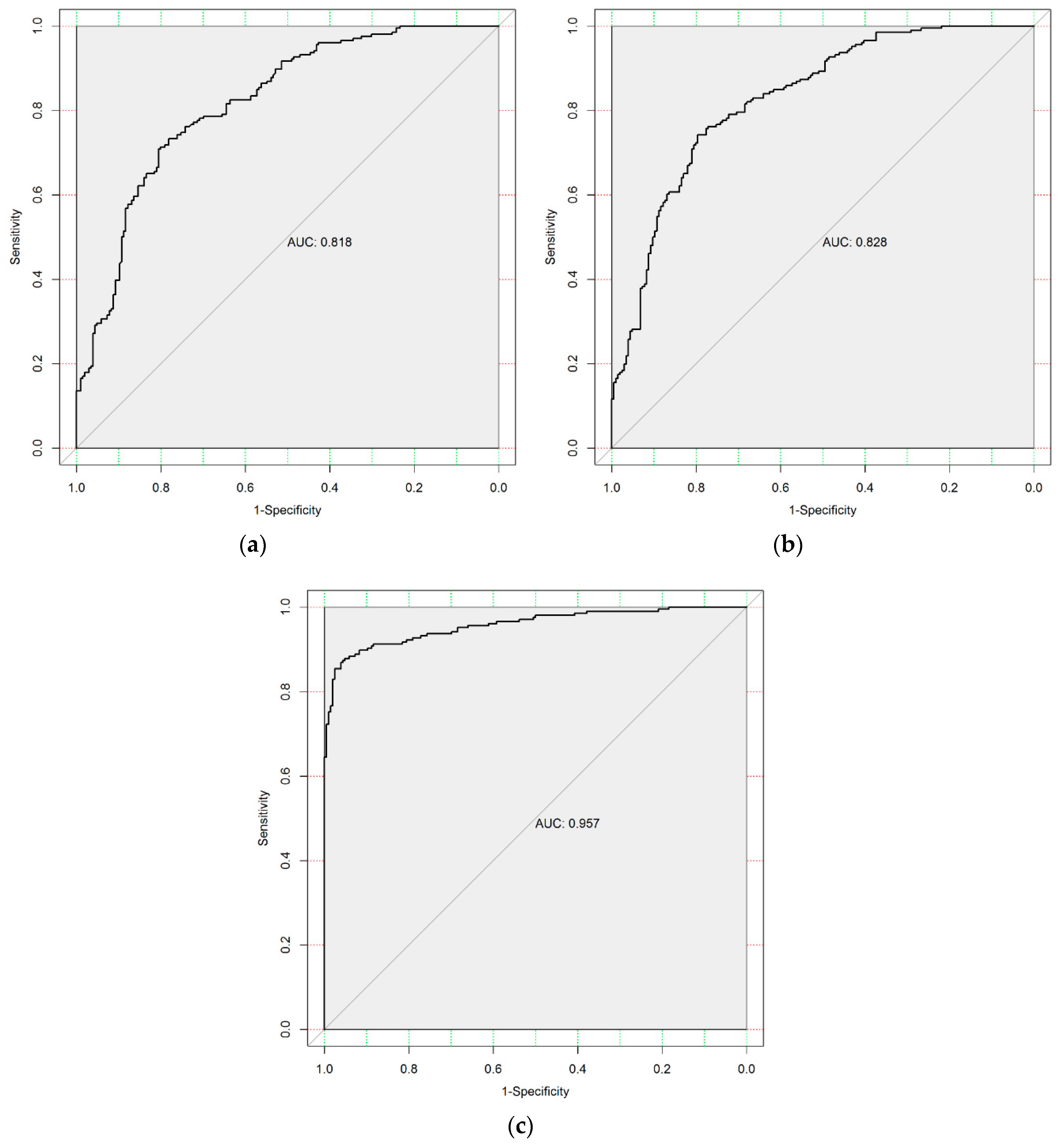
4.2.1. Model Performance

As shown in

Table 8. The performance metrics of three regression models.

Parameter	LR	ALR	ESFLR
TN	157	160	191
FN	49	46	15
FP	55	52	24
TP	151	154	182
Positive accuracy (%)	73.30	74.76	88.35
Negative accuracy (%)	76.21	77.67	92.72
Overall accuracy (%)	74.76	76.21	90.53
AUC	0.818	0.828	0.957
Nagelkerke R2	0.3907	0.4075	0.7810
AIC	440.31	426.86	236.08

, the performance metrics of the three constructed models were obtained. The highest positive accuracy, which indicates the rate of correctly classifying the landslide points into each landslide class, is 88.35 for the ESFLR model, followed by the ALR (74.76) and LR (73.30) models. For the negative accuracy, which indicates the proportion of non-landslide points classified into the non-landslide class, the ESFLR model has the highest value of 92.72, followed by the ALR (77.67) and LR (76.21) models. The overall accuracy measures the overall classification ability of the models, and the value is 90.53 for the ESFLR model, 76.21 for the ALR model, and 74.76 for the LR model. These results clearly suggest that the ESFLR model is superior to the other two models in terms of classification accuracy for both landslides and non-landslides. The ESFLR model yielded an improved overall accuracy, which was 18.79% higher than the ALR model and 21.09% higher than the LR model.

In this study, the ROC curve acts as a graphical indicator to measure the overall performance of the three models. As Figure 5 conceptually illustrates, the AUC values of the LR model, the ALR model and the ESFLR model are 0.818, 0.828 and 0.957, respectively. Compared with the LR model and the ALR model, the ESFLR model exhibited better performance. Furthermore, the ESFLR model with a higher Nagelkerke R² (0.7810) and a lower AIC value (236.08) showed a better goodness of fit compared with the LR model and the ALR model (Table 8).

4.2.2. Detection of Spatial Autocorrelation of Residuals

Table 9. Moran’s I values of the residuals in the three regression models.

Model	Moran’s I	p Value
LR	0.4104	<0.001
ALR	0.3971	<0.001
ESFLR	0.0270	0.1558

summarizes the Moran’s I values of the three models, which were used to detect the spatial autocorrelation among residuals. The Moran’s I values were 0.4104, 0.3971 and 0.0270 for the LR model, the ALR model and the ESFLR model, respectively. Among the three models, the residuals of both the LR model and the ALR model showed obvious positive spatial autocorrelation, indicating that the two models suffer from a misspecification problem. The spatial autocorrelation of residuals of the ALR model was only slightly reduced compared to the LR model. The introduction of the autocovariate term did not play a role in this study. In contrast, the Moran’s I value of the ESFLR model was reduced to 0.0270, indicating that the residuals of the ESFLR model are not spatially autocorrelated. This result proved that the addition of a linear combination of eigenvectors effectively eliminated the negative effect of spatial autocorrelation on the model.

4.2.3. Cross Validation

A 10-fold cross validation was adopted in this study, and the average results of 10 runs, including the negative accuracy, the positive accuracy and the overall accuracy, for both the training dataset and validation dataset were obtained (

Table 10. The average results of 10-fold cross validation.

Model	Training Dataset			Validation Dataset
	Negative Accuracy (%)	Positive Accuracy (%)	Overall Accuracy (%)	Negative Accuracy (%)	Positive Accuracy (%)	Overall Accuracy (%)
LR	77.24	73.25	75.24	76.74	72.69	74.70
ALR_90	77.89	74.86	76.37	77.69	74.17	75.92
ESFLR	90.18	90.24	90.21	88.33	89.88	89.10

). The results of cross validation indicate that each model exhibits a similar performance for its training dataset and validation dataset, suggesting that the three models all have a certain generalization capacity. A pairwise comparison between the three models shows that the ESFLR model has the best overall performance.

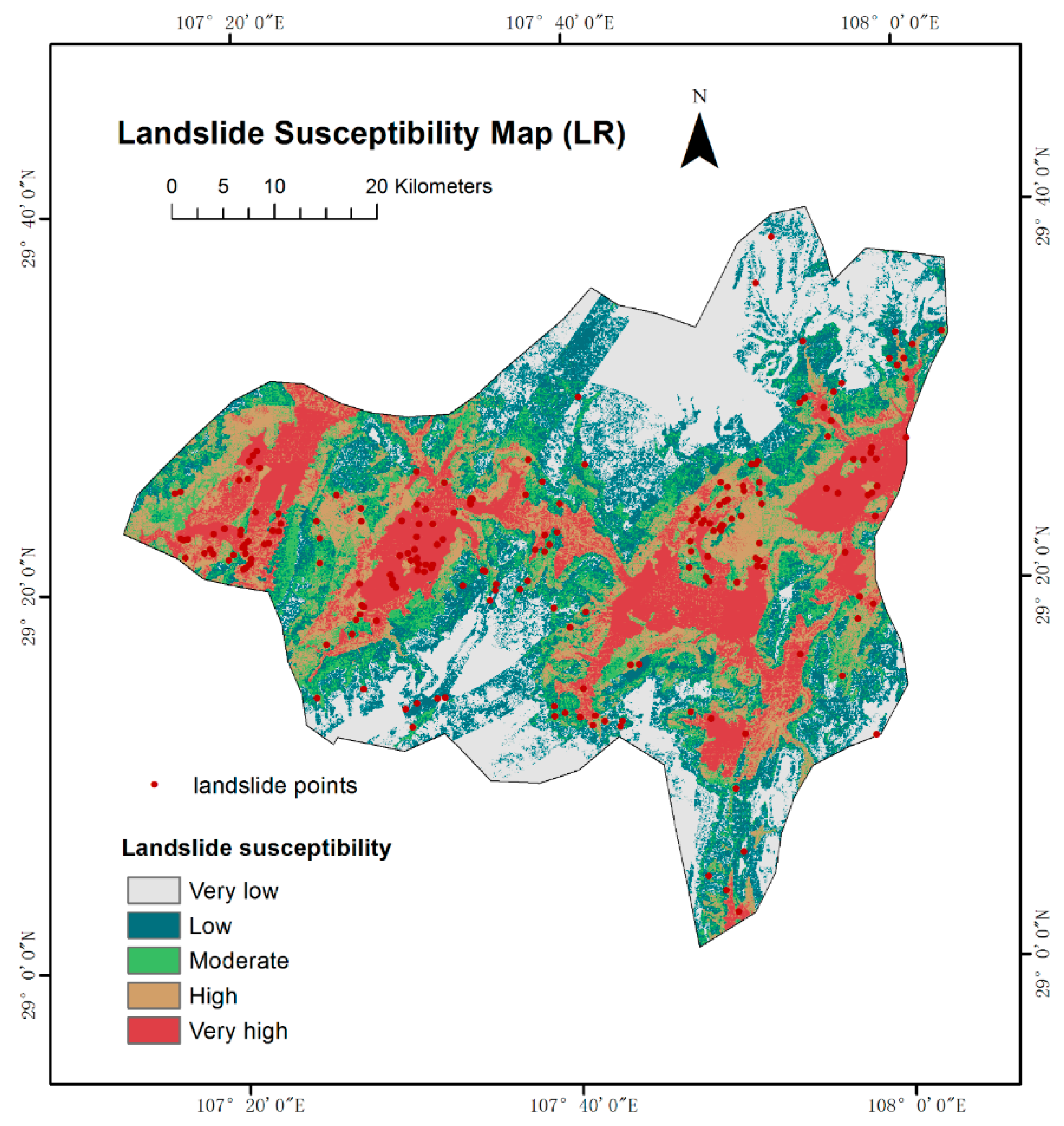
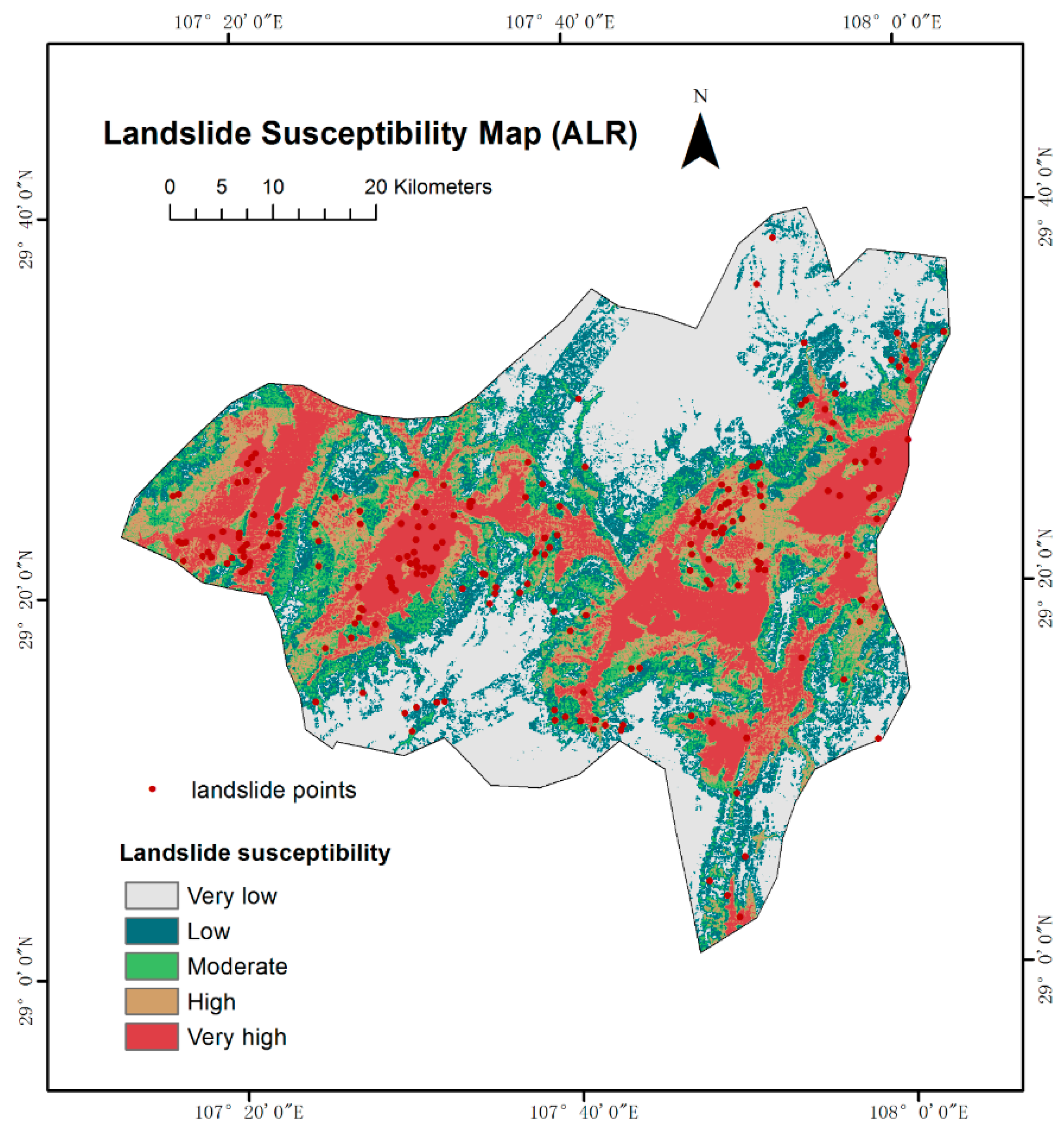
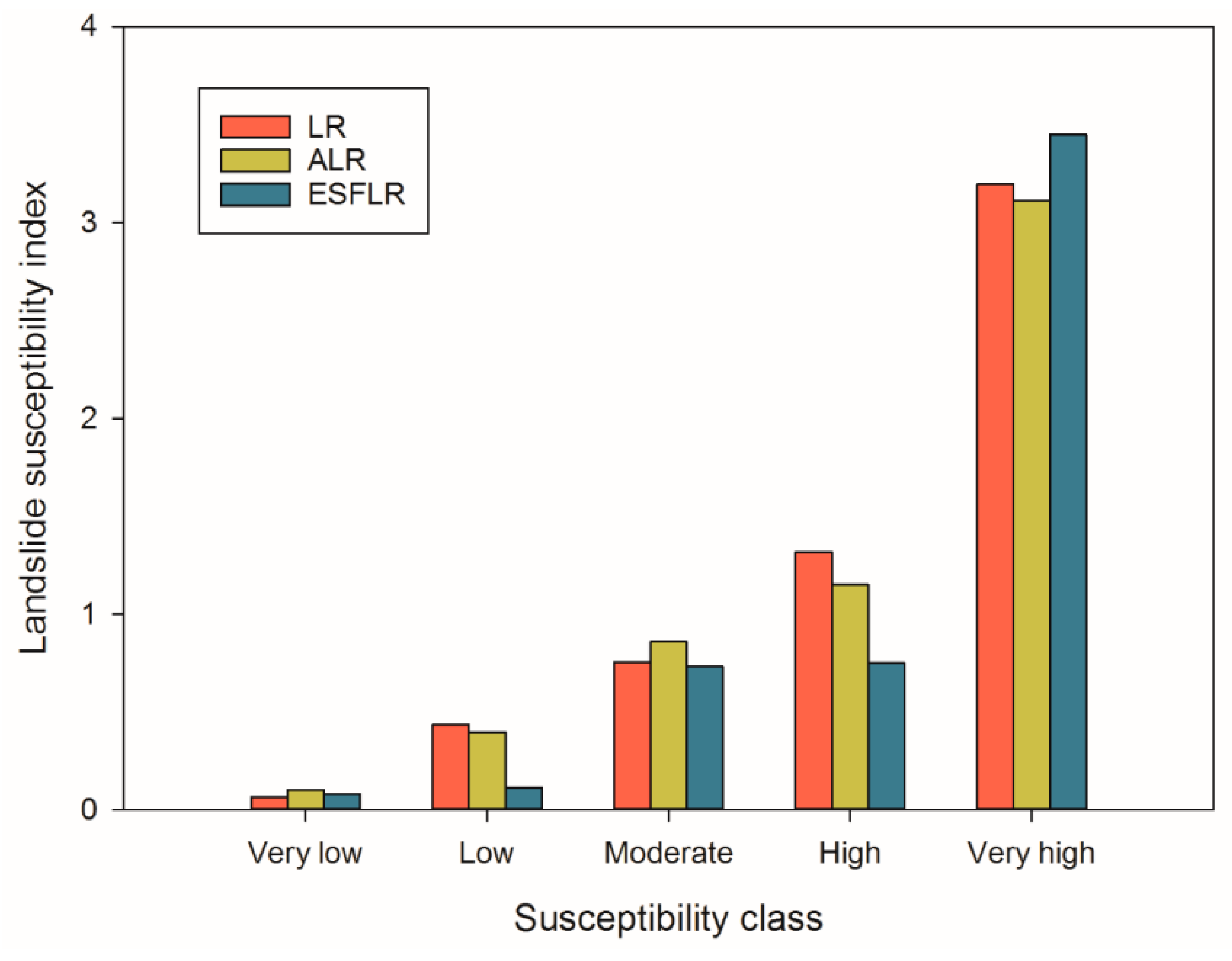
4.3. Landslide Susceptibility Mapping

Landslide susceptibility mapping is necessary for disaster management and development planning. Based on the LR, ALR and ESFLR models, the landslide susceptibility values, i.e., the possibility of landslide occurrence were computed. Based on natural breaks, which is a classification method that is generally used for statistical mapping, the landslide susceptibility values were categorized into five classes: very high, high, moderate, low and very low. The landslide susceptibility maps were thus prepared by using the three regression models, and these maps were superimposed with the landslide inventory points, as shown in Figure 6, Figure 7 and Figure 8. We calculated statistics for each landslide susceptibility class (

Table 11. Validation of landslide susceptibility maps obtained by the LR, ALR and ESFLR models.

Model	Susceptibility Class	Landslide	Landslide Area (m2)	% Landslide Covered (a)	% Area Covered (b)	Landslide Density (a/b)
LR	Very high	90	3,561,500	55.94	17.51	3.19
	High	47	1,254,800	19.71	14.96	1.32
	Moderate	34	837,650	13.16	17.42	0.76
	Low	29	596,200	9.36	21.65	0.43
	Very low	6	116,900	1.84	28.47	0.06
ALR	Very high	101	3,947,200	61.99	19.92	3.11
	High	41	955,350	15.00	13.05	1.15
	Moderate	30	763,400	11.99	13.95	0.86
	Low	25	474,200	7.45	18.75	0.40
	Very low	9	226,900	3.56	34.33	0.10
ESFLR	Very high	148	4,937,650	77.55	22.48	3.45
	High	27	585,700	9.20	12.27	0.75
	Moderate	14	531,800	8.35	11.45	0.73
	Low	6	116,600	1.83	15.98	0.11
	Very low	11	195,300	3.07	37.81	0.08

).

The results of the LR model (Figure 6) showed that the very high susceptibility areas were mainly distributed in the western, eastern and central parts of the study area, while the very low susceptibility areas were in the northern and southwestern parts. The very high susceptibility areas occupied 17.51% of the study area, followed by a value of 14.96% for the high susceptibility areas, and the moderate, low and very low susceptibility areas occupied 17.42%, 21.65%, and 28.47%, respectively. The ALR model showed similar results to the LR model (Figure 7), but the former had relatively clustered landslide susceptibility zonation with smoother and clearer edges. A total of 19.92% of the study area was classified as very high susceptibility, and 13.05% was classified as high susceptibility. The moderate, low and very low susceptibility areas accounted for 13.95%, 18.75%, and 34.33%, respectively. The ESFLR model yielded different results compared with the other two models: the proportion of very high susceptibility areas was higher (Figure 8), reaching 22.48%, and the consistency with the landslide inventory points was significantly increased. The percentage values for the high, moderate, low and very low susceptibility areas were 12.27%, 11.45%, 15.98% and 37.81%, respectively.

For landslide prediction, an effective model should not only achieve high classification accuracy but should also ensure that more landslide points fall into the limited landslide-prone area to effectively determine the real landslide-prone area, and provide support for land resource allocation. Therefore, we exploited the landslide density index, which is defined as the ratio between the percentage of the landslide covered area (the landslide area in each susceptibility class zone) and the percentage of the total area covered (the area of each susceptibility class zone) to assess the quality of the landslide susceptibility maps. The landslide density indexes of the very high susceptibility class in the LR, ALR and ESFLR models were 3.19, 3.11 and 3.45, respectively. The ESFLR model had the highest value and performed better than the other two models. As shown in Figure 9, the landslide density index of each model increased with the increase in landslide susceptibility, which indicated that the distribution of evaluation results fit well with that of the landslide inventory points. The results of the ESFLR model indicated that the proportions of the number and the area of landslide inventory points that fell into the very high and high susceptibility areas reached 84.95% and 86.75%, respectively, while the proportions of the number and the area of the landslide inventory points that fell into the very low and low susceptibility areas were only 8.25% and 4.90%, respectively. The three landslide susceptibility maps indicate that the high landslide risk areas tend to be distributed in the low elevation areas. This result may be because the study area is mountainous, and the low elevation areas with frequent human activities and intensive infrastructure construction are more prone to landslides.

As demonstrated in this study, the ESFLR model offers several advantages for landslide susceptibility mapping. With a linear combination of eigenvectors selected as additional independent variables, the map patterns of the response variables remaining within the residuals can be effectively explained, eliminating the spatial autocorrelation of the residuals of the ESFLR and improving the overall performance of the model. Thus, the method may also be helpful when the available landslide disposing factors are insufficient to explain all map patterns in the response variables.

However, this method still has some limitations. The method is computationally demanding and involves eigen-decomposition and stepwise selection of eigenvectors. The computation requirements will greatly increase with the increase in the number of landslide samples, which takes extensive time and means the method is not applicable for large-scale landslide data or real-time landslide risk warning. In addition, based on this method, it is difficult to directly determine whether a landslide disposing factor contributes positively or negatively to landslide occurrence.

5. Conclusions

Because the residuals in conventional logistic regression display strong spatial autocorrelation, a model misspecification problem may occur. The ESFLR model was constructed for landslide susceptibility assessment by introducing eigenvector spatial filtering into conventional logistic regression to explain the spatial patterns of the dependent variables inherent in the model residuals. The results demonstrated that the ESFLR model worked well in eliminating the spatial autocorrelation among residuals, and its performance improved significantly compared to the other two regression models. Furthermore, by verifying the landslide susceptibility maps for the three models, the ESFLR model provided a map that had the best consistency with landslide inventory data. This work demonstrated that the ESFLR model was an effective, reasonable and flexible method for dealing with spatial autocorrelation of residuals, which has often been neglected in previous landslide research. Mathematically, the ESFLR model is also a safe, reliable and stable method.

Strong spatial autocorrelation in model residuals may not only be a result of model misspecification, but may also be due to insufficient independent variables that cannot account for all spatial patterns in the dependent variable. Some significant variables may be missing from the model specification. Further research should explore additional factors other than those in our graphs, e.g., land use and rainy seasonal precipitation, which can be added during model specification to explain the remaining spatial patterns in the dependent variable. In addition, the influence of the selection method of non-landslide points should be discussed in a further study, and more effective methods may be applied. Some of the data used here may be slightly imprecise due to data accessibility; however, more appropriate data are not currently available. We will continue to look for better data sources in further research. Considering the limitations of the ESFLR method for large-scale landslide data due to the computational demands, we consulted with other scholars and determined that the segmented processing approach [47] or fast-ESF method [48] might be helpful, which will be evaluated in our subsequent research.

References

1. Dai, F.C.; Lee, C.F.; Ngai, Y.Y. Landslide risk assessment and management: An overview. Eng. Geol. 2002, 64, 65–87. [Google Scholar] [CrossRef]
2. Bai, S.B.; Wang, J.; Lü, G.N.; Zhou, P.G.; Hou, S.S.; Xu, S.N. GIS-based logistic regression for landslide susceptibility mapping of the Zhongxian segment in the Three Gorges area, China. Geomorphology 2010, 115, 23–31. [Google Scholar] [CrossRef]
3. Atkinson, P.M.; Massari, R. Generalised linear modelling of susceptibility to landsliding in the central apennines, italy. Comput. Geosci. 1998, 24, 373–385. [Google Scholar] [CrossRef]
4. Budimir, M.E.A.; Atkinson, P.M.; Lewis, H.G. A systematic review of landslide probability mapping using logistic regression. Landslides 2015, 12, 419–436. [Google Scholar] [CrossRef] [Green Version]
5. Che, V.B.; Kervyn, M.; Suh, C.E.; Fontijn, K.; Ernst, G.G.J.; Marmol, M.A.D.; Trefois, P.; Jacobs, P. Landslide susceptibility assessment in Limbe (SW Cameroon): A field calibrated seed cell and information value method. Catena 2012, 92, 83–98. [Google Scholar] [CrossRef]
6. Ba, Q.; Chen, Y.; Deng, S.; Wu, Q.; Yang, J.; Zhang, J. An Improved Information Value Model Based on Gray Clustering for Landslide Susceptibility Mapping. ISPRS Int. J. Geo Inf. 2017, 6, 18. [Google Scholar] [CrossRef]
7. Ba, Q.; Chen, Y.; Deng, S.; Yang, J.; Li, H. A comparison of slope units and grid cells as mapping units for landslide susceptibility assessment. Earth Sci. Inform. 2018, 11, 373–388. [Google Scholar] [CrossRef]
8. Lee, S.; Pradhan, B. Landslide hazard mapping at Selangor, Malaysia using frequency ratio and logistic regression models. Landslides 2007, 4, 33–41. [Google Scholar] [CrossRef]
9. Zhang, G.; Cai, Y.; Zheng, Z.; Zhen, J.; Liu, Y.; Huang, K. Integration of the Statistical Index Method and the Analytic Hierarchy Process technique for the assessment of landslide susceptibility in Huizhou, China. Catena 2016, 142, 233–244. [Google Scholar] [CrossRef]
10. Fan, X.Y.; Qiao, J.P.; Chen, Y.B. Application of analytic hierarchy process in assessment of typical landslide danger degree. J. Nat. Disasters 2004, 13, 72–76. [Google Scholar]
11. Lee, S.; Ryu, J.H.; Won, J.S.; Park, H.J. Determination and application of the weights for landslide susceptibility mapping using an artificial neural network. Eng. Geol. 2004, 71, 289–302. [Google Scholar] [CrossRef]
12. Zare, M.; Pourghasemi, R.H.; Vafakhah, M.; Pradhan, B. Landslide susceptibility mapping at Vaz Watershed (Iran) using an;artificial neural network model: A comparison between multilayer;perceptron (MLP) and radial basic function (RBF) algorithms. Arab. J. Geosci. 2013, 6, 2873–2888. [Google Scholar] [CrossRef]
13. Xu, C.; Dai, F.; Xu, X.; Yuan, H.L. GIS-based support vector machine modeling of earthquake-triggered landslide susceptibility in the Jianjiang River watershed, China. Geomorphology 2012, 145–146, 70–80. [Google Scholar] [CrossRef]
14. Brenning, A. Spatial prediction models for landslide hazards: Review, comparison and evaluation. Nat. Hazards Earth Syst. Sci. 2005, 5, 853–862. [Google Scholar] [CrossRef]
15. Lee, S. Application of logistic regression model and its validation for landslide susceptibility mapping using GIS and remote sensing data. Int. J. Remote Sens. 2005, 26, 1477–1491. [Google Scholar] [CrossRef]
16. Yilmaz, I. Landslide susceptibility mapping using frequency ratio, logistic regression, artificial neural networks and their comparison: A case study from Kat landslides (Tokat—Turkey). Comput. Geosci. 2009, 35, 1125–1138. [Google Scholar] [CrossRef]
17. Akgun, A. A comparison of landslide susceptibility maps produced by logistic regression, multi-criteria decision, and likelihood ratio methods: A case study at İzmir, Turkey. Landslides 2012, 9, 93–106. [Google Scholar] [CrossRef]
18. Tobler, W.R. A Computer Movie Simulating Urban Growth in the Detroit Region. Econ. Geogr. 1970, 46, 234–240. [Google Scholar] [CrossRef]
19. Getis, A. A History of the Concept of Spatial Autocorrelation: A Geographer’s Perspective. Geogr. Anal. 2010, 40, 297–309. [Google Scholar] [CrossRef]
20. Erener, A.; Düzgün, H. Improvement of statistical landslide susceptibility mapping by using spatial and global regression methods in the case of More and Romsdal (Norway). Landslides 2010, 7, 55–68. [Google Scholar] [CrossRef]
21. Getis, A. Screening for spatial dependence in regression analysis. Pap. Reg. Sci. Assoc. 1990, 69, 69–81. [Google Scholar] [CrossRef]
22. Getis, A. Spatial Filtering in a Regression Framework: Examples Using Data on Urban Crime, Regional Inequality and Government Expenditures; Springer: Berlin, Germany, 2010; pp. 172–185. [Google Scholar]
23. Griffith, D.A. A linear regression solution to the spatial autocorrelation problem. J. Geogr. Syst. 2000, 2, 141–156. [Google Scholar] [CrossRef]
24. Getis, A.; Griffith, D.A. Comparative Spatial Filtering in Regression Analysis. Geogr. Anal. 2002, 34, 130–140. [Google Scholar] [CrossRef]
25. Ayalew, L.; Yamagishi, H.; Marui, H.; Kanno, T. Landslides in Sado Island of Japan: Part II. GIS-based susceptibility mapping with comparisons of results from two methods and verifications. Engi. Geol. 2005, 81, 432–445. [Google Scholar] [CrossRef]
26. Wang, Q.; Wang, D.; Yong, H.; Wang, Z.; Zhang, L.; Guo, Q.; Wei, C.; Sang, M. Landslide Susceptibility Mapping Based on Selected Optimal Combination of Landslide Predisposing Factors in a Large Catchment. Sustainability 2015, 7, 16653–16669. [Google Scholar] [CrossRef] [Green Version]
27. Dai, F.C.; Lee, C.F. Landslide characteristics and slope instability modeling using GIS, Lantau Island, Hong Kong. Geomorphology 2002, 42, 213–228. [Google Scholar] [CrossRef]
28. Eeckhaut, M.V.D.; Reichenbach, P.; Guzzetti, F.; Rossi, M. Combined landslide inventory and susceptibility assessment based on different mapping units: An example from the Flemish Ardennes, Belgium. Nat. Hazards Earth Syst.Sci. NHESS Discuss. NHESSD 2009, 9, 507–521. [Google Scholar] [CrossRef]
29. Pourghasemi, H.R.; Pradhan, B.; Gokceoglu, C. Application of fuzzy logic and analytical hierarchy process (AHP) to landslide susceptibility mapping at Haraz watershed, Iran. Nat. Hazards 2012, 63, 965–996. [Google Scholar] [CrossRef]
30. Wang, Q.; Li, W.; Wu, Y.; Pei, Y.; Xie, P. Application of statistical index and index of entropy methods to landslide susceptibility assessment in Gongliu (Xinjiang, China). Environ. Earth Sci. 2016, 75, 599. [Google Scholar] [CrossRef]
31. Schaefer, R.L. Alternative estimators in logistic regression when the data are collinear. J. Stat. Comput. Simul. 1986, 25, 75–91. [Google Scholar] [CrossRef]
32. Miles, J. Tolerance and Variance Inflation Factor; John Wiley and Sons: Hoboken, NJ, USA, 2005; pp. 2055–2056. [Google Scholar]
33. Allison, P.D. Logistic Regression Using the SAS System: Theory and Application; SAS Publishing: Cary, NC, USA, 1999. [Google Scholar]
34. Griffith, D.A.; Peresneto, P.R. Spatial modeling in ecology: The flexibility of eigenfunction spatial analyses. Ecology 2006, 87, 2603–2613. [Google Scholar] [CrossRef]
35. Griffith, D.A. Spatial Autocorrelation and Spatial Filtering; Springer: Berlin/Heidelberg, Germany, 2013; pp. 633–635. [Google Scholar]
36. Thayn, J.B.; Simanis, J.M. Accounting for Spatial Autocorrelation in Linear Regression Models Using Spatial Filtering with Eigenvectors. Ann. Assoc. Am. Geogr. 2013, 103, 47–66. [Google Scholar] [CrossRef]
37. Dormann, C.; McPherson, J.; Araújo, M.; Bivand, R.; Bolliger, J.; Carl, G.; Wilson, R. Methods to Account for Spatial Autocorrelation in the Analysis of Species Distributional Data: A Review. Ecography 2007, 30, 609–628. [Google Scholar] [CrossRef]
38. Atkinson, P.M.; Massari, R. Autologistic modelling of susceptibility to landsliding in the Central Apennines, Italy. Geomorphology 2011, 130, 55–64. [Google Scholar] [CrossRef]
39. Augustin, N.H.; Ma, B.S.M. An autologistic model for the spatial distribution of wildlife. J. Appl. Ecol. 1996, 33, 339–347. [Google Scholar] [CrossRef]
40. Hong, H.; Pradhan, B.; Xu, C.; Bui, D.T. Spatial prediction of landslide hazard at the Yihuang area (China) using two-class kernel logistic regression, alternating decision tree and support vector machines. Catena 2015, 133, 266–281. [Google Scholar] [CrossRef]
41. Frattini, P.; Crosta, G.; Carrara, A. Techniques for evaluating the performance of landslide susceptibility models. Eng. Geol. 2010, 111, 62–72. [Google Scholar] [CrossRef]
42. García-Rodríguez, M.J.; Malpica, J.A.; Benito, B.; Díaz, M. Susceptibility assessment of earthquake-triggered landslides in El Salvador using logistic regression. Geomorphology 2008, 95, 172–191. [Google Scholar] [CrossRef] [Green Version]
43. Peng, C.Y.J.; Lee, K.L.; Ingersoll, G.M. An introduction to logistic regression analysis and reporting. J. Educ. Res. 2002, 96, 3–14. [Google Scholar] [CrossRef]
44. Tiefelsdorf, M. The Saddlepoint Approximation of Moran’s I’s and Local Moran’s Ii’s Reference Distributions and Their Numerical Evaluation. Geogr. Anal. 2002, 34, 187–206. [Google Scholar] [CrossRef]
45. Bengio, Y.; Grandvalet, Y. Bias in Estimating the Variance of K-Fold Cross-Validation; Springer: New York, NY, USA, 2005; pp. 75–95. [Google Scholar]
46. Fushiki, T. Estimation of Prediction Error by Using K-fold Cross-Validation; Kluwer Academic Publishers: Berlin/Heidelberg, Germany, 2011; pp. 137–146. [Google Scholar]
47. Yang, J.; Chen, Y.; Chen, M.; Yang, F.; Yao, M. A Segmented Processing Approach of Eigenvector Spatial Filtering Regression for Normalized Difference Vegetation Index in Central China. ISPRS Int. J. Geo Inf. 2018, 7, 330. [Google Scholar] [CrossRef]
48. Murakami, D.; Griffith, D.A. Eigenvector Spatial Filtering for Large Data Sets: Fixed and Random Effects Approaches. Geogr. Anal. 2019, 51, 23–49. [Google Scholar] [CrossRef]
Figure 1. Position and landslide inventory map of the study area.
Ijgi 08 00332 g001
Figure 2. Maps of landslide predisposing factors: (a) elevation; (b) slope; (c) aspect; (d) curvature; (e) distance to road; (f) distance to railway; (g) distance to river; (h) distance to fault; (i) precipitation; (j) lithology; (k) normalized difference vegetation index (NDVI).
Ijgi 08 00332 g002aIjgi 08 00332 g002bIjgi 08 00332 g002c
Figure 3. The Thiessen polygons of the landslide point dataset.
Ijgi 08 00332 g003
Figure 4. Moran’s I values of the eigenvectors.
Ijgi 08 00332 g004
Figure 5. The ROC curves: (a) the LR model; (b) the ALR model; (c) the ESFLR model.
Ijgi 08 00332 g005
Figure 6. Landslide susceptibility map for the LR model.
Ijgi 08 00332 g006
Figure 7. Landslide susceptibility map for the ALR model.
Ijgi 08 00332 g007
Figure 8. Landslide susceptibility map for the ESFLR model.
Ijgi 08 00332 g008
Figure 9. Landslide susceptibility index in susceptibility classes.
Ijgi 08 00332 g009