Investigating the Spatiotemporally Varying Correlation between Urban Spatial Patterns and Ecosystem Services: A Case Study of Nansihu Lake Basin, China

Abstract

Ecosystem services are the benefits obtained from an ecosystem that have great significance in sustainable development. Urbanization has triggered significant changes on urban spatial patterns, which have had a great impact on the ecosystem services. However, studies on the spatiotemporally varying relationship between urban spatial patterns and ecosystem services are lacking. Taking as a case study, the Nansihu Lake Basin in China, this study aimed to explore the spatiotemporally varying relationship between urban spatial patterns and ecosystem services. Urban spatial patterns were derived by integrating remote sensing and spatial metrics. Ecosystem service values were calculated using ecosystem service models. The spatiotemporally varying impact of urban spatial patterns on ecosystem services was quantified using the Geographically Weighted Regression (GWR) model. The findings indicate that urban spatial patterns and ecosystem services have dramatically varied with the urbanization process. The estimated parameters indicate that urban spatial patterns have significant impacts on ecosystem services. The GWR revealed a spatiotemporally varying correlation and improved the explanatory ability in comparison with the Ordinary Least Squares (OLS) model. The investigation of the impact of urban spatial patterns on ecosystem services can provide more practical support for effective urban planning and ecosystem management.

1. Introduction

Ecosystem services refer to life-supporting products and services, directly or indirectly obtained from the structure, process, and function of ecosystems that form and maintain environmental conditions and utility for human survival and development [1]. Ecosystem services are mainly composed of four types, namely, supporting, provisioning, regulating, and cultural services that form the basis for regional ecological security and sustainable development, as well as being the key to human well-being. It has been reported that nearly two thirds of global ecosystem services have been damaged as a result of human activity [2]. Recent decades have witnessed dramatic urbanization around the world; this trend is expected to be one of the vital issues of global change in the future, with urban land expected to increase from 0.65 million km² in 2000 to 1.86 million km² in 2030 [3]. The urbanization process has a profound impact on land use by transforming non-urban land into urban land. Although urbanization can improve society and benefit economic development, changes in land use caused by urbanization dramatically affect ecosystem services on a global scale by influencing the interactions between the hydrosphere, atmosphere, and biosphere [4,5]. This is crucial for urban planning and sustainable development because land use changes have irreversible and long-term effects. In addition, the increasing populations that accompany urbanization require a greater supply of ecosystem services [6].

Under such circumstances, effectively evaluating the impact of land use changes on ecosystem services has become a matter of global concern, and it is urgently required to provide support for policy making that could mitigate its negative effects on the ecology and promote regional sustainable development [7]. Since the implementation of the Millennium Ecosystem Assessment (MEA) project in 2001, an increasing number of studies have been conducted that demonstrate that urbanization induced land use change is becoming a significant contributor of variation in ecosystem services [6,8]. Variations in land use structures directly influence ecosystem service dynamics, while variations in land use patterns indirectly influence them through changing ecological processes [9]. However, previous studies have only focused on investigating the relationship between ecosystem services and land use structure [10,11]. How ecosystem services respond to changes in land use patterns has not been fully characterized, and the quantitative relationship between land use patterns and ecosystem services is poorly understood. To assess how changes in spatial patterns affect ecosystem services, exploring the relationship between ecosystem services and spatial patterns is important.

Previous studies have analyzed entire study areas to investigate the impact of land use changes on ecosystem services, ignoring the existing spatial heterogeneities [12,13]. However, significant spatial dependence is normally involved in the relationship between land use and ecosystem services because complex ecosystems components are correlated and affected by energy, material, and information flow [6,14]. A large number of studies found that urbanization is negatively correlated with ecosystem services. However, certain scholars have noted that ecosystem services are enhanced during urbanization. Zhou et al. (2018) found that urban expansion had a positive impact on ecosystem services values in the Beijing-Tianjin-Hebei region during the period of 1996–2014 [15]. Buyantuyev and Wu (2009) demonstrated that net primary productivity (NPP) increased in Phoenix, United States, during the urbanization process [16]. The cited studies indicate that the impact of urban land use changes on ecosystem services significantly varies over space, which can be due to the fact that changes in urban land and ecosystem services are highly related to local environmental and socioeconomic conditions. Global impact only reflects average conditions and might consequently ignore local-specific impacts. If we overlooked the spatial heterogeneity that can induce errors in statistical analysis of the impacts of related factors on ecosystem services, uncertainty in decisions regarding the management of ecosystem services might increase [17]. In addition, investigating the relationship between spatial patterns of urban land and changes in ecosystem services for single temporal data overlooks the fact that the direction and magnitude of the impact could shift along with the urbanization process. Therefore, the impact on ecosystem services cannot be fully investigated, which could hinder effective urban planning.

Adopting the Nansihu Lake Basin (NLB), China as study area, this research aims to examine the relationship between urban spatial patterns and ecosystem services in rapid urbanization regions through the integration of multi-temporal remote sensing images, spatial metrics, InVEST model [18], and the Geographically Weighted Regression (GWR) model. The specific study objectives are (1) to characterize the dynamics of urban spatial patterns from 1995 to 2015 in the NLB; (2) to reveal the spatiotemporal distribution of ecosystem services values from 1995 to 2015; and (3) to investigate the impact of urban spatial patterns on ecosystem services with consideration of spatiotemporal heterogeneities.

2. Materials and Methods

2.1. Study area and Data Sources

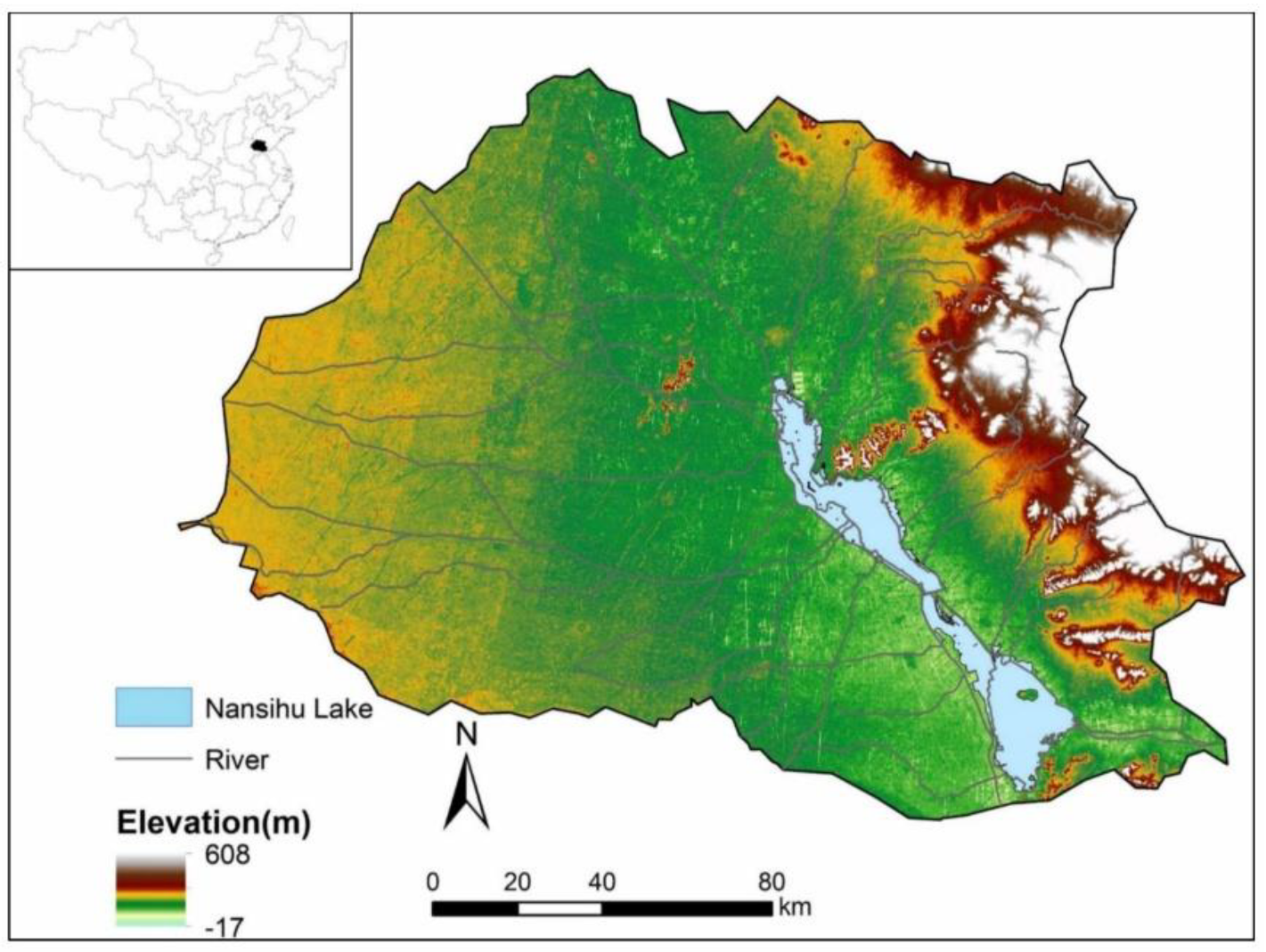
As shown in Figure 1, Nansihu Lake (116°34′-117°21′E, 34°27′-35°20′N) is located at the junction of 4 provinces (Shandong, Anhui, Henan, Jiangsu) in eastern China. It is the largest freshwater lake in northern China. The total area of the Nansihu Lake Basin (NLB) is 28,364 km². It has a semi-humid monsoon continental climate, with an average annual temperature of 14.2 °C, an average annual precipitation of 750 mm, and an annual potential evapotranspiration of 942 mm [19]. The NLB is not only a main impounded lake for the South-to-North Water Diversion Project in China [20], but also an important natural reservoir in eastern China. The main land use types include built-up land, agricultural land, forest, grassland, and water body. Since the 1980s, the NLB has undergone significant urbanization and rapid socio-economic development. Between 1995 and 2015, the rate of urban population grew from 57.5% to 87.2% in the NLB. Meanwhile, gross domestic product (GDP) rose from 120 billion to 1540 billion yuan. The NLB’s rapid urbanization has resulted in the serious degradation of ecosystem services, put pressure on the environment, and increased competition for land resources. The NLB faces difficulties in achieving regional sustainable development, needing to balance urbanization and ecosystem services. Thus, it is crucial to analyze the spatiotemporal heterogeneity of urban spatial patterns and ecosystem services, and their relationship in the NLB. The analysis result could contribute to realizing the "win-win" goal of socioeconomic development and ecology protection in the NLB.

We used remote sensing data as well as meteorological, socioeconomic, geographic ancillary, and statistical data in this study. Specifically, (1) Landsat TM images for 1995, 2005, and Landsat OLI images for 2015 under clear sky conditions, obtained from the Geospatial Data Cloud (http://www.gscloud.cn). Detailed information of the remote sensing data is provided in

Table 1. List of Landsat images.

Year	Path	Row	Acquisition Date
1995	121	35	26 March 1995
	121	36	11 April 1995
	122	35	17 March 1995
	122	36	04 May 1995
	123	35	09 April 1995
	123	36	11 May 1995
2005	121	35	24 May 2005
	121	36	24 May 2005
	122	35	13 April 2005
	122	36	13 April 2005
	123	35	04 April 2005
	123	36	04 April 2005
2015	121	35	25 September 2015
	121	36	25 September 2015
	122	35	02 October 2015
	122	36	02 October 2015
	123	35	09 October 2015
	123	36	09 October 2015

. To avoid the negative effects on remote sensing classification, atmospheric correction and radiometric normalization were carried out. (2) Considering the significance of ecosystem services and data availability for the basin, we chose 4 types of ecosystem services, namely, water yield, soil conservation, carbon storage, and crop production. Meteorological data (annual average precipitation, monthly precipitation and temperature) from 56 meteorological stations in and around the basin were collected from the National Meteorological Information Center (http://data.cma.cn). The meteorological data were further interpolated into 30 m resolution images using the Inverse Distance Weighted (IDW) method [21]. (3) Digital Elevation Model (DEM) data with a resolution of 30 m were collected from the United States Geological Survey (http://www.usgs.gov). (4) Soil property data were collected from the China Soil Map-Based Harmonized World Soil Database (v1.1) (http://westdc.westgis.ac.cn). (5) Normalized Difference Vegetation Index (NDVI) data for 1995 were collected from the GIMMS-NDVI dataset. NDVI data, for 2005 and 2015 were derived from MOD13A1 (http://modis.gsfc.nasa.gov/data/). (6) Statistical crop production data were collected from the China County Statistical Yearbook [22,23,24]. All spatial data were projected to the Universal Transverse Mercator (UTM) coordinate system.

2.2. Urban Spatial Pattern Analysis

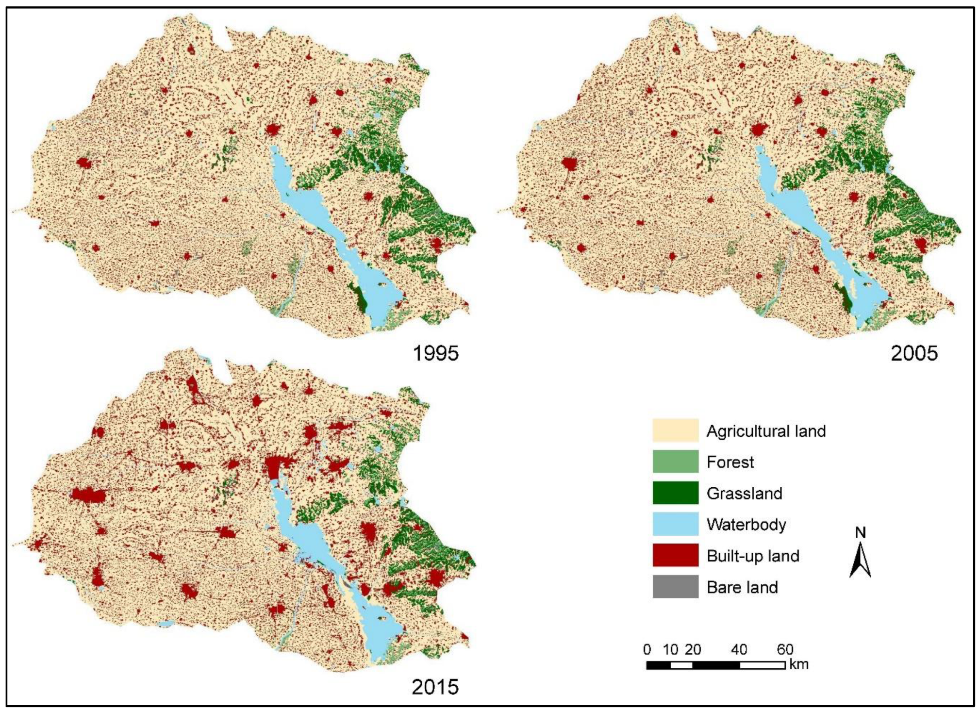
Given the current situation of the NLB and the spectral characteristics of Landsat images, 6 land use categories were identified, namely, agricultural land, built-up land, forest, grassland, waterbody, and bare land. The Maximum Likelihood Classifier (MLC), which is one of the most widely used classification methods, was applied to conduct supervised classification of the Landsat images. Signatures obtained from 500 training sample points were developed for each time point according to a field survey data acquired in 1995 and 2005, and Google Earth acquired in 2015. After classification, a commonly used 3 × 3 majority filter was further applied to improve the classified results by removing salt and pepper effects.

For each land use map, 500 reference points were produced using stratified random sampling to evaluate the accuracy of the classification. A confusion matrix was developed, and overall accuracies and the Kappa statistic were calculated based on the error matrix.

To reveal the dynamics of the urban spatial pattern in the NLB, several spatial metrics at class level were computed using Fragstats 4.2 [25]. Based on the research objective and previous studies, four spatial metrics were selected: percentage of landscape (PLAND), patch density (PD), edge density (ED), and mean shape index (SHAPE_MN). These metrics can effectively quantify the composition, fragmentation, and irregularity of the urban spatial pattern in the NLB [26].

PLAND is used to quantify the percentage of built-up land for each statistical sample. It is positively related to the degree of urbanization. PD is a simple metric reflecting the number of built-up land patches per spatial unit, which can provide information on the fragmentation of built-up land. ED represents the density of all edge segments of built-up land. ED increases when patch shapes become more complex. SHAPE_MN measures the irregularity of built-up land patches. When a landscape is composed of a single square patch SHAPE_MN=1. The increase in SHAPE_MN value implies that the landscape shape becomes more irregular [25].

In this study, the calculation of spatial metrics was initially conducted for the entire area to gain a general overall understanding of the spatial patterns of built-up land over the whole study area. The NLB was further divided into multiple grids for localizing the dynamics of urban spatial patterns and exploring their impacts on ecosystem services. Based on the local condition and the commonly used grid sizes in previous stduies, a preliminary test with grid sizes of 2 km, 5 km, 8 km, and 10 km was implemented to analyze the scale effects on spatial analysis. The grid size of 5 km was finally chosen based on considerations of information retention and redundancy, and computing efficiency. A finer grid size could result in only a few patches or no patch existing in certain grids, which produces redundancy in analysis. A coarser grid size could omit detailed information regarding the spatial pattern and ecosystem services. A grid size of 5 km enabled us to detect the heterogeneity and improve the computing efficiency of finer scales. The selected landscape metrics for each grid were further calculated to reveal the spatiotemporal patterns of urban land on the local level. After obtaining the multiple temporal spatial metrics values, change ratio of the metrics values were computed according to Equation (1):

$$M{C}_i^k=\frac{M_{i,t+n}^k-M_{i,t}^k}{M_{i,t}^k},$$

(1)

where $M_{i,t+n}^k$ and $M_{i,t}^k$ represent the value of spatial metric $k$ in year $t+n$ and $t$, respectively. $M{C}_i^k$ is the change ratio of spatial metric $k$ for grid $i$.

2.3. Quantification of Ecosystem Services

Four types of ecosystem services were selected and estimated in this study: water yield, soil conservation, carbon storage and crop production. These ecosystem services were selected with consideration of the following criteria: (1) ecosystem services play a key role in achieving sustainable development in the NLB; (2) ecosystem services are strongly relevant to human well-being and are affected by urbanization in the study area [6,10]; (3) models for calculating ecosystem services are available and the data required to run the model is available. Ecosystem service values were calculated using land use data derived from Landsat images, soil property data, meteorological data, DEM data, statistical crop production data and NDVI data.

Water yield is defined as the amount of water from the different parts of a landscape in the InVEST model. Annual water yield ($Y_x$) for pixel x can be quantified according to the water balance principle using the following equation:

$$Y_x=\left(1-\frac{AE{T}_x}{P_x}\right)\times p_x,$$

(2)

where $p_x$ denotes the average annual precipitation for pixel x, and $AE{T}_x$ represents the actual annual evapotranspiration for pixel x.

Soil erosion is considered as one of the important drivers of land degradation and the loss of limited cropland. Therefore, the Revised Universal Soil Loss Equation (RUSLE) was adopted to estimate the capacity of soil conservation for each pixel, which can be calculated using Equation (3):

$$S{C}_x=A{p}_x-A{r}_x,$$

(3)

where $S{C}_x$ is the amount of soil conservation at pixel $x$, $A{p}_x$ and $A{r}_x$ represent the amount of potential and the actual soil loss, respectively. $A{p}_x$ and $A{r}_x$ can be expressed as follows:

$$A{p}_x=R_x\times K_x\times L_x\times S_x,$$

(4)

$$A{r}_x=R_x\times K_x\times L_x\times S_x\times C_x\times P_x,$$

(5)

where $R_x$ is the rainfall erosion index for pixel $x$, $K_x$ represents the soil erosion factor for pixel x, $L_x$ indicates the slope length factor, $S_x$ denotes the slope for pixel $x$, $C_x$ and $P_x$ represent the cover-management factor and the support practices factor, respectively. $C_x$ and $P_x$ are assigned 1, if there is no vegetation or support practice for pixel $x$. In this study, $C_x$ and $P_x$ shown in

Table 2. Cover-management factor (C) and support practice factor (P) values.

Land Use Type	C	P
Agricultural land	0.3	0.4
Forest	0.003	0.2
Grassland	0.01	0.2
Waterbody	0.003	0.2
Built-up land	0.001	0.001
Bare land	0.01	0.2

were determined according to the relevant literature [27].

The total amount of carbon storage in the NLB was quantified on the basis of the 4 types of carbon density (aboveground mass carbon density, belowground mass carbon density, soil organic mass carbon density and dead organic mass carbon density) and the land use maps. In this study, carbon storage $C_{x,y,p}^{total}$ for pixel $x$ with land use category p can be expressed as follows:

$$C_{x,p}^{total}=A{S}_x\times \left(C{D}_p^{above}+C{D}_p^{below}+C{D}_p^{soil}+C{D}_p^{dead}\right),$$

(6)

where $A{S}_x$ represents the area of pixel $x$ and $C{D}_p^{above}$, $C{D}_p^{below}$, $C{D}_p^{soil}$, and $C{D}_p^{dead}$ indicate the carbon density of the different carbon pools for land use category p, respectively. The carbon density values were obtained according to previous studies and are presented in

Table 3. Carbon density values in the Nansihu Lake Basin (NLB) (Mg/hm²).

Land Use Type	Aboveground Carbon Density	Belowground Carbon Density	Soil Organic Carbon Density	Dead Organic Carbon Density
Agricultural land	5.7	0.7	92.6	0
Forest	42.4	10.8	120.8	7.8
Grassland	0.7	2.8	111.1	0
Waterbody	0	0	0	0
Built-up land	0	0	0	0
Bare land	0.1	0	9.6	0

. It was assumed that carbon storage for built-up land is negligible and it was set to zero based on the study by Sun & Li (2017) [27].

Because a significant linear relationship exists between crop production and the NDVI value for agricultural land type [28], in this study, the county level statistical data on crop production were allocated to each grid of agricultural land by using the NDVI value. The maximum value of the NDVI in agricultural land that reflects the best growth status was derived, and crop production for each pixel was estimated as follows:

$$Cro{p}_{x,i}=\frac{NDV{I}_{x,i}}{NDV{I}_{sum,i}}\times Cro{p}_{c,i},$$

(7)

where $Cro{p}_{x,i}$ is the crop production for agricultural land pixel $x$ in county $i$. $NDV{I}_{x,i}$ and $NDV{I}_{sum,i}$ represent the maximum NDVI value for pixel $x$ and the overall NDVI value for agricultural land in county $i$, respectively. $Cro{p}_{c,i}$ is the overall crop production value in county $i$, which was obtained from the statistical yearbook [22,23,24].

2.4. Regression Analysis

Understanding how the urban spatial pattern has contributed to ecosystem services is crucial for effective urban planning and ecosystem management. Spatial regression analysis has been widely used to explore the correlation between dependent and explanatory variables. For comparison purposes, the Ordinary Least Squares (OLS) regression and GWR models were applied to examine the relationship between ecosystem services and urban spatial patterns in this study. OLS is a type of linear least squares method for estimating the unknown parameters in a linear regression model. OLS chooses the parameters of a linear function of a set of explanatory variables by the principle of least squares. It can be expressed by Equation (8) [29]:

$$y={\alpha }_0+{\displaystyle \sum }_k{\alpha }_k{x}_k+\epsilon ,$$

(8)

where $y$ represents the dependent variable, ${\alpha }_0$ indicates the intercept value, ${\alpha }_k$ represents the coefficient for the $k$ th explanatory variable $x_k$, and $\epsilon$ denotes the random error term. Using all data samples to fit one model, OLS is a global regression model. Parameters including ${\alpha }_0$ and ${\alpha }_k$ remain fixed in space.

However, the relationship between urbanization and ecosystem services may vary spatially because of the study area’s local context. Differences in urban spatial patterns could result in variations in ecosystem services. OLS only globally estimates the average relationship for all samples when analyzing phenomena that have spatial variation. Spatial nonstationarity cannot be incorporated into an OLS model [30].

Rather than estimating a single global parameter, the GWR model generates a set of local parameters to reflect the spatial nonstationarity of the model at different locations. The parameters can be applied to achieve a better insight into the relationship between dependent and explanatory variables by examining the spatially varying relationships.

The GWR model can be expressed as follows [31]:

$$y_i=a_0\left({\mu }_i,v_i\right)+{{\displaystyle \sum }}_k{a}_k\left({\mu }_i,v_i\right)x_{ik}+{\epsilon }_i,$$

(9)

where $y_i$ is the dependent variable of the sample unit $i$, (${\mu }_i,v_i$) indicates the spatial coordinates of the sample unit $i$, $a_0\left({\mu }_i,v_i\right)$ is the intercept value for sample unit $i$, $a_k\left({\mu }_i,v_i\right)$ denotes the local coefficient estimate for explanatory variable $x_{ik}$, and ${\epsilon }_i$ represents the error term for sample unit $i$. In Equation (9), the estimates for the parameters are spatially nonstationary.

Parameters for sample unit $i$ in the GWR model can be derived by weighting all samples around sample unit $i$ with respect to distance, which is calculated in terms of the Euclidean distance [32]. The samples closer to sample unit $i$ have a stronger impact on the estimation of the local parameter, and are assigned larger weights than for distant samples. The Gaussian distance decay function is applied to set the weights:

$$w_{ij}=\exp (\frac{d_{ij}^2}{h^2}),$$

(10)

where $w_{ij}$ represents the weight of sample unit $j$ for its neighborhood sample unit $i$, $d_{ij}$ is the Euclidean distance between sample unit $i$ and unit $j$, $h$ corresponds to the kernel bandwidth. Weight equals one when the distance between sample unit $i$ and unit $j$ is zero. Weight rapidly approaches 0 when kernel bandwidth $h$ is smaller than distance $d_{ij}$.

Two kernel types in the GWR model are widely used to compute weights: the fixed and the adaptive kernel type. In this study, the fixed kernel type was selected because the density of the sample units is uniform. In addition, parameters estimated from the GWR model are also sensitive to the kernel bandwidth. Three methods can be used to determine kernel bandwidth: Bandwidth Parameter (BP), corrected Akaike Information Criterion (AICc), and Cross Validation (CV) [32]. BP can be used when the kernel bandwidth is known. Otherwise, the AICc and CV methods should be used to identify the optimal kernel bandwidth. In this study, the kernel bandwidth is not provided. Therefore, the identification of the bandwidth was based on the AICc method because of its potential to minimize the AICc value.

The explanatory abilities of the OLS and GWR models were compared and analyzed using three statistical indicators. Adjusted R² and AICc measure a model’s degree of goodness of fit [30]. The larger that the adjusted R² is, the stronger the ability of the explanatory variable to explain the variances of the dependent variables. Additionally, a smaller AICc value means that the model results are closer to the actual values. Moran’s I value was further calculated for the residuals of OLS and GWR models to quantify the models’ capacity to support the variables spatial autocorrelation. Moran’s I value, range from -1 to 1, it is widely used to represent the degree of spatial autocorrelation. An absolute value of Moran’s I closer to 1 suggests the existence of significant spatial autocorrelation. An absolute value of Moran’s I closer to 0 implies perfect spatial randomness.

3. Results

3.1. Change in Urban Spatial Patterns

Remote sensing images during the period of from 1995 to 2015 were classified into six land use types using Environment for Visualizing Images software (ENVI, version 5.1). The overall accuracies of the classified data were 88%, 92%, and 90%, with corresponding Kappa statistics of 0.87, 0.91, and 0.88 for 1995, 2005, and 2015, respectively, which implies that classification was adequate. Figure 2 shows the distribution of land use from 1995 to 2015 in the NLB. Forest land and grassland were mainly located in the eastern part of the basin. Growth in built-up land was mainly observed around the existing city core as well as on the suburban areas. Area statistics data for each land use type are presented in

Table 4. Land use statistics in the NLB for 1995, 2005, and 2015.

		Agricultural Land	Forest	Grassland	Waterbody	Built-up Land	Bare Land
1995	Area (km2)	20,475.94	753.14	1408.04	1609.50	3990.47	127.35
	Percent (%)	72.19	2.66	4.96	5.67	14.07	0.45
2005	Area (km2)	20,373.68	676.34	1371.51	1537.32	4288.39	117.20
	Percent (%)	71.83	2.38	4.84	5.42	15.12	0.41
2015	Area (km2)	19,674.02	437.05	1044.72	1670.12	5463.27	75.26
	Percent (%)	69.36	1.54	3.68	5.89	19.26	0.27

. Agricultural land was the predominant land use type in the NLB during the study period, followed by built-up land and waterbody. Built-up land expanded at a rapid pace, with the area increasing from 3990.47 km² in 1995 to 5463.27 km² in 2015. This expansion suggests that the NLB has experienced rapid urbanization over the period. Conversely, substantial pressure caused by the rapid increase of built-up land on other land use types was reflected by the decrease in agricultural land, forest, grassland, and bare land. Among these land use types, agricultural land and grassland experienced the highest decreases: 801.92 km² and 363.32 km², respectively. Furthermore, it is found that the growth rate of urban land between 1995 and 2005 is smaller than that between 2005 and 2015. Over the period 1995-2005, built-up land expansion was mainly constrained by relatively low economic level and insufficient infrastructure in the NLB. During the period 2005-2015, rapid industrialization and urbanization resulted in the rising demand for built-up land, thus much agricultural land has been converted into built-up land, and the extent of the city core continued to increase. On the other hand, because of the deepening urbanization and flexible population mobility policy, an increase in in-migration and natural population has led to rapid population growth in the city. As a result, the conflict between limited land resource and rapid urban sprawl became more apparent.

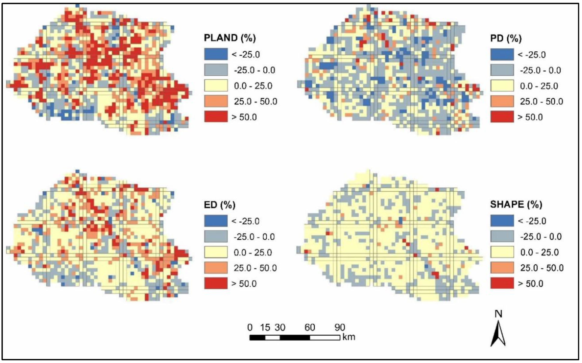
As a result of the rapid urbanization in the NLB, land use change has triggered a remarkable variation in urban spatial patterns. Landscape metrics can provide a detailed insight into the impacts of urbanization on landscape fragmentation and complexity [33]. In this study, landscape patterns of built-up land were quantified based on the four selected metrics: PLAND, PD, ED, SHAPE_MN.

Table 5. Spatial metrics values of built-up land for 1995, 2005, and 2015.

Year	PLAND	PD	ED	SHAPE_MN
1995	14.0738	0.6182	13.3492	1.1715
2005	15.1244	0.6003	13.7626	1.1904
2015	19.2576	0.5907	15.0949	1.2254

presents the spatial metrics values of built up land for 1995, 2005 and 2015 in the NLB. The increase in ED and SHAPE_MN indicate the increasing complexity of urban patches. The change ratio of spatial metrics values at local scale were further calculated according to Equation 1. As shown in Figure 3, the spatial pattern of built-up land in the NLB varied spatiotemporally during the urbanization process.

The PLAND value increased from 14.0738 to 19.2576, which is in accordance with statistical data shown in Table 4. The spatial pattern of variation in PLAND indicates that the allocation of new built-up land included both growth around the existing city core and the generation of new built-up land patches. Since the implementation of market-oriented reform in China, cities have experienced significant urbanization. Compared with the period 1995–2005, the annual rate of growth in PLAND was greater over the period 2005–2015, which indicates NLB experienced rapid urban growth process with the accelerating speed over the study period. The economy of NLB was moving into the fast lane. Rapid development required more built-up land and industrial workers than ever before, which also led to relatively high urbanization speed. In addition, because of limited land resources in the city core, the hotspot of urban growth moved from the city core to urban fringes and the neighboring rural areas. PD can be used to measure how fragmented the spatial pattern of built-up land is. At the global level, PD decreased from 0.6182 to 0.5907, which indicates that the number of urban patches declined during the period under analysis. This can be attributed to the fact that some isolated urban patches are connected to generate a larger patch due to urban expansion. As shown in Figure 3, PD dramatically increased in urban fringes and rural areas, and decreased in the city cores. The increase in PD can be mainly attributed to the conversion from non-built-up land into built-up land, which made the landscape more fragmented. ED value increased from 13.3492 to 15.0949 between 1995 and 2015. In detail, the rate of change from 2005 to 2015 is much greater than the rate of change between 1995 and 2005. This can be explained by the fact that the development cores grew together to form more irregular patches over the period 2005–2015. The noticeable increase in ED implies diffuse urban sprawl development pattern in the NLB. Although ED variation in the city core was not obvious, urban fringes experienced significant increases in ED, which indicates that patch shapes became more irregular. This outcome could be attributed to the fact that existing built-up patches merged and generated larger but more regular patches in the city core, while a dispersal of new urban development made the built-up land pattern more irregular. Along with the rapid urbanization, a more complicated urban landscape formed, as indicated by the increase in SHAPE_MN.

3.2. Dynamics of Ecosystem Services

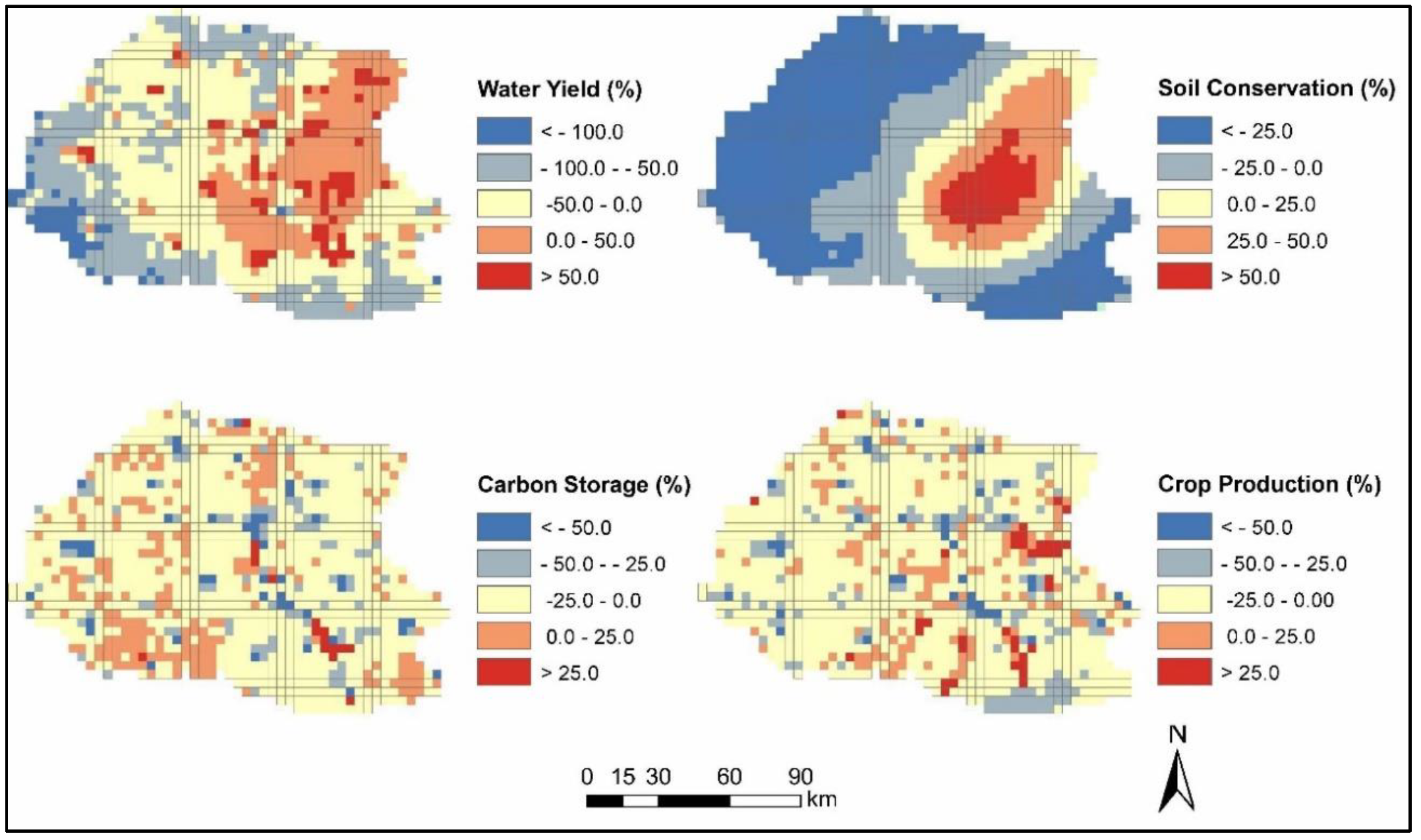
Quantity statistics for ecosystem services in the NLB are presented in

Table 6. Ecosystem services values in the NLB from 1995 to 2015.

Ecosystem Services	1995	2005	2015	1995–2015 Change Ratio (%)
Water Yield (m3)	14,680,789.29	14,055,285.79	13,256,121.71	9.70
Soil Conservation (tons)	3,102,891.63	2,991,353.39	2,978,579.24	4.01
Carbon Storage (tons)	51,980,021.35	51,637,304.90	48,075,172.51	7.51
Crop Production (tons)	3,796,203.80	3,642,626.29	3,429,217.75	9.67

. Results reveal that the amount of the four ecosystem services decreased by 9.70%, 4.01%, 7.51%, and 9.67%, respectively from 1995 to 2015. Due to the more significant built-up land expansion and spatial pattern change over the period 2005–2015, the decrease rates of water yield, carbon storage, and crop production over the period 2002–2015 is greater than those over the 1995–2005. Compared with the other three ecosystem services, the different trend of change in soil conservation can be partly due to the climate factor, for example the precipitation factor. The precipitation is negatively related to the soil conservation value [34]. As shown in Figure 4, dramatic spatial variations of the selected ecosystem services could be observed in the NLB.

Water yield decreased from 14,680,789.29 m³ to 13,256,121.71 m³ during the study period. Regarding spatial variation in water yield changes, the city core had the higher value because evapotranspiration of lower vegetation coverage increased water yield there. The highest reduction occurred in the western region.

The total value of soil conservation decreased from 3,102,891.63 tons to 2,978,579.24 tons. With regards to the spatial distribution of changes in soil conservation, the eastern area performed better than the other areas. A continuous area in the western part of the NLB also experienced considerable degradation, which can be explained by the fact that the western part experienced a rapid urbanization process. Agricultural and vegetation land were converted into built-up land. Significant increase in soil conservation was observed in the eastern part of the NLB.

During the rapid urbanization process, the total carbon storage in the NLB decreased from 51,980,021.35 tons in 1995 to 48,075,172.51 tons in 2015. As shown in Figure 4, the increase in carbon storage values was mainly located in the rural area, which is covered by agricultural land, forest and grassland with higher carbon density. By contrast, major reductions in carbon storage were mainly observed in the city core and significant growing built-up areas. The reduction in total carbon storage value can be explained by the reduction in agricultural land, forest, and grass land as well as the growth in built-up land. The decrease in total carbon storage indicates that the carbon sequestration regulating service decreased.

During the urbanization process, agricultural land was converted into built-up land. Degradation in agricultural land led to a direct decrease in crop production in the NLB. Crop production decreased from 3,796,203.80 tons in 1995 to 3,429,217.75 tons in 2015. In the new urban expansion area, agricultural land was transformed into built-up land, so crop production reduced by 100%.

3.3. Relationship between Urban Spatial Patterns and Ecosystem Services

To investigate the relationship between urban spatial patterns and ecosystem services, the OLS and GWR models were used. The OLS model could only produce a global coefficient for the study area, while coefficients produced by the GWR model varied over space. The adjusted R² and AICc values of these two models are presented in

Table 7. Comparison of R² between the Geographically Weighted Regression (GWR) and Ordinary Least Squares (OLS) models.

Year	Spatial Metrics	Water Yield		Soil Conservation		Carbon Storage		Crop Production
		GWR	OLS	GWR	OLS	GWR	OLS	GWR	OLS
1995	PLAND	0.909	0.418	0.736	0.178	0.782	0.209	0.665	0.182
	PD	0.879	0.264	0.731	0.162	0.762	0.147	0.674	0.196
	ED	0.900	0.293	0.758	0.196	0.773	0.164	0.641	0.171
	SHAPE_MN	0.567	0.127	0.582	0.027	0.519	0.080	0.613	0.100
2005	PLAND	0.914	0.405	0.725	0.169	0.783	0.176	0.678	0.126
	PD	0.881	0.211	0.717	0.153	0.757	0.152	0.686	0.139
	ED	0.895	0.227	0.752	0.160	0.756	0.134	0.644	0.110
	SHAPE_MN	0.591	0.134	0.581	0.078	0.523	0.108	0.510	0.094
2015	PLAND	0.906	0.369	0.737	0.164	0.832	0.204	0.701	0.195
	PD	0.805	0.192	0.688	0.033	0.748	0.085	0.675	0.174
	ED	0.807	0.106	0.731	0.158	0.726	0.127	0.623	0.183
	SHAPE_MN	0.509	0.115	0.546	0.080	0.671	0.075	0.529	0.105

and

Table 8. Comparison of the Akaike Information Criterion (AICc) between GWR and OLS models.

Year	Spatial Metrics	Water Yield		Soil Conservation		Carbon Storage		Crop Production
		GWR	OLS	GWR	OLS	GWR	OLS	GWR	OLS
1995	PLAND	11259	13953	8714	10090	9576	11092	21898	22950
	PD	11614	13736	8746	10182	9671	11114	21871	22986
	ED	11319	13466	8588	10119	9572	11108	21973	22963
	SHAPE_MN	12865	13697	9599	10186	10663	11025	22559	22854
2005	PLAND	11363	13094	8670	10257	9542	11069	21797	22890
	PD	11777	13516	8715	10192	9680	11181	21775	22931
	ED	11564	13370	8530	9845	9625	11047	21899	22957
	SHAPE_MN	12983	13815	9503	10824	10629	11238	22486	22974
2015	PLAND	11331	13555	8644	10019	9466	11032	21699	22893
	PD	12268	13925	8826	10068	9955	11313	21794	22905
	ED	12247	13804	8618	9998	10095	11312	21984	22857
	SHAPE_MN	13081	13790	9382	10073	10895	11304	22486	22854

. As indicated by the lower R² and higher AICc values, the OLS model was poorly fitted in all cases for different time points. The adjusted R² for the GWR model ranged from 0.914 to 0.509, which implies that the impacts of urban spatial patterns on ecosystem services are better explained with the GWR model, given the higher goodness of fit. Moreover, AICc values generated by the GWR model were smaller than those generated by the OLS model, suggesting that the GWR model helps to better explain the impacts of urban spatial patterns on ecosystem services.

Furthermore,

Table 9. Comparison of Moran’s I between GWR and OLS models.

Year	Spatial Metrics	Water Yield		Soil Conservation		Carbon Storage		Crop Production
		GWR	OLS	GWR	OLS	GWR	OLS	GWR	OLS
1995	PLAND	−0.054	0.585	−0.075	0.536	−0.064	0.632	−0.033	0.505
	PD	0.012	0.716	−0.058	0.572	0.016	0.626	0.028	0.550
	ED	0.001	0.702	−0.063	0.547	−0.018	0.634	0.018	0.523
	SHAPE_MN	0.046	0.713	0.046	0.581	0.044	0.551	0.038	0.508
2005	PLAND	−0.047	0.624	−0.082	0.571	−0.055	0.612	−0.009	0.526
	PD	0.025	0.719	−0.020	0.523	0.031	0.587	0.030	0.522
	ED	0.019	0.703	−0.037	0.544	0.034	0.610	0.024	0.549
	SHAPE_MN	0.042	0.655	0.048	0.590	0.069	0.596	0.025	0.537
2015	PLAND	−0.022	0.763	−0.080	0.564	−0.020	0.630	−0.002	0.567
	PD	0.048	0.674	−0.009	0.578	0.044	0.587	0.038	0.548
	ED	0.073	0.664	−0.019	0.549	0.037	0.596	0.048	0.513
	SHAPE_MN	0.038	0.654	0.035	0.582	0.044	0.578	0.038	0.533

shows Moran’s I values for the residuals of these two models. Significant positive spatial autocorrelation was revealed as shown by the Moran’s I values generated by the OLS model ranging from 0.505 to 0.763. Furthermore, the lower Moran’s I values generated by the GWR model when compared against those generated by the OLS model, indicate the GWR model is more reliable for explaining the spatial autocorrelation of the variables under investigation.

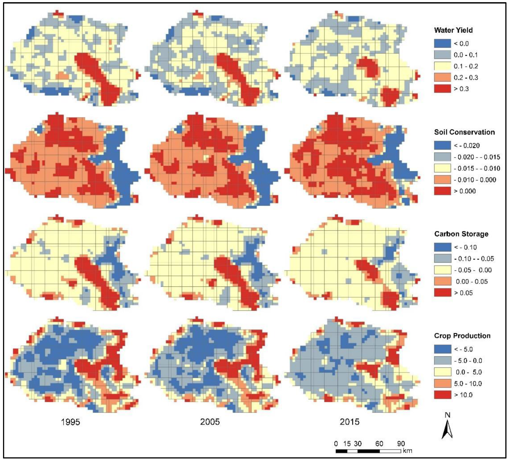
The spatial distribution of coefficients shown in Figure 5, Figure 6, Figure 7 and Figure 8 suggest that the relationship between the four spatial metrics and selected ecosystem service types changed with the variation of spatial position. Both the positive and negative impacts of urban spatial patterns on ecosystem services were observed.

The adjusted R² values of the correlation between PLAND and the four ecosystem services indicate that PLAND had a significant impact on the changes in ecosystem services. Figure 5 shows a clear spatial distribution of the coefficients between the PLAND of built-up land and the four ecosystem services. Similarly, significant positive correlations between PLAND and water yield were found in most of the study area. In addition, negative correlation between PLAND and soil conservation was detected in the eastern area of the NLB, suggesting that the increase in the built-up land resulted in a reduction of the soil conservation. The area with a positive correlation increased during the urbanization process. A negative effect on the carbon storage value was observed in the NLB, which indicates that urban expansion caused the reduction in carbon storage. Additionally, Figure 5 implies that urban expansion had a negative impact on crop production in a large part of the study area, although positive coefficients were found in the eastern area of the NLB. PLAND could explain more than 65% of the variation in ecosystem services in the NLB as evidenced by Table 7.

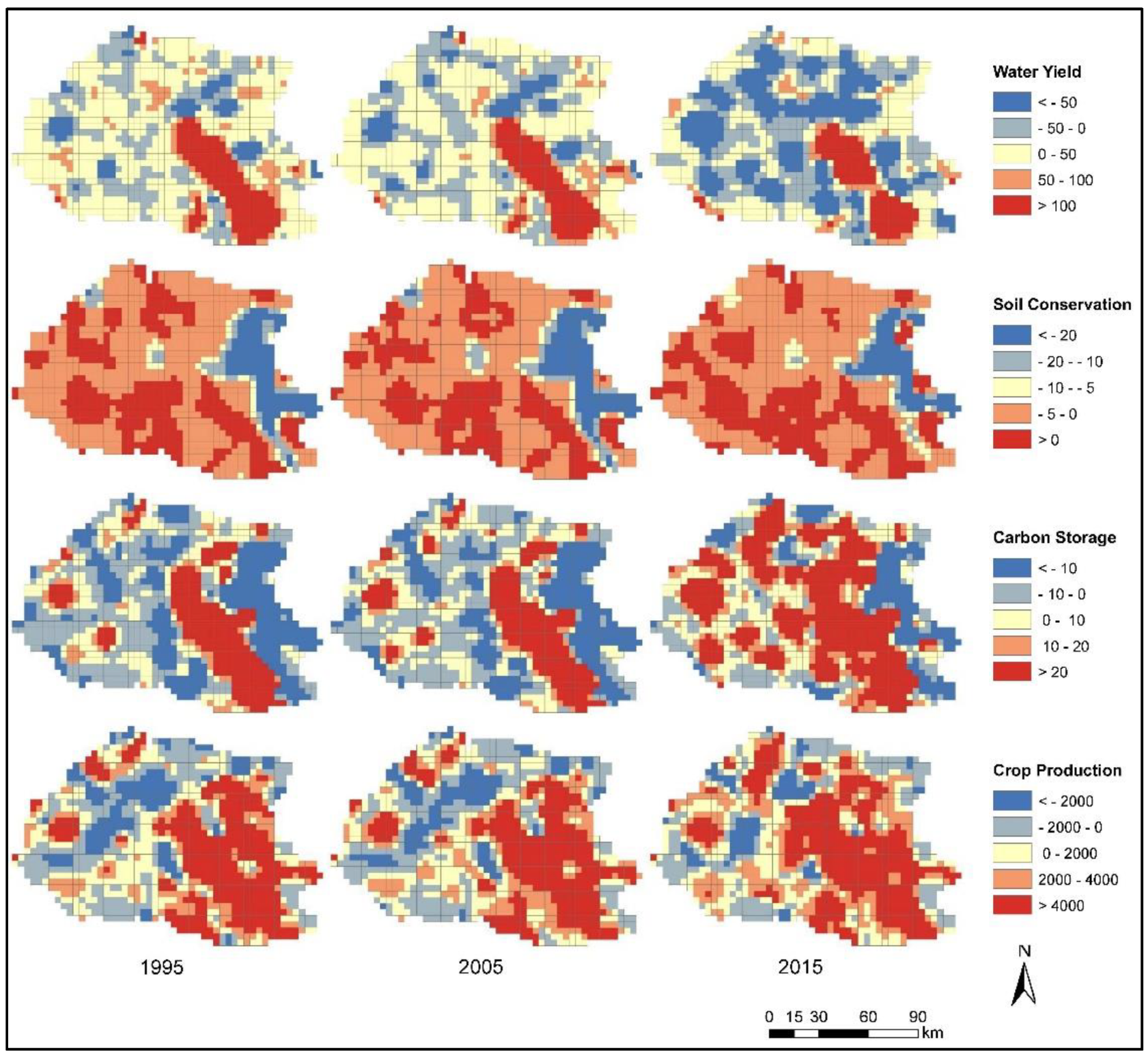
Furthermore, the spatio-temporally varying impacts of PD on ecosystem services was revealed. As shown in Table 7, water yield and PD exhibited high correlation. PD explained 87.9% 88.1%, and 80.5% of the variations in water yield value for 1995, 2005, and 2015, respectively. Both positive and negative correlations were found in the results estimated with the GWR model. Figure 6 presents a clear cluster in the correlations. More significant positive impact was observed in the city core and fringe areas while lower correlation was observed in the rural areas.

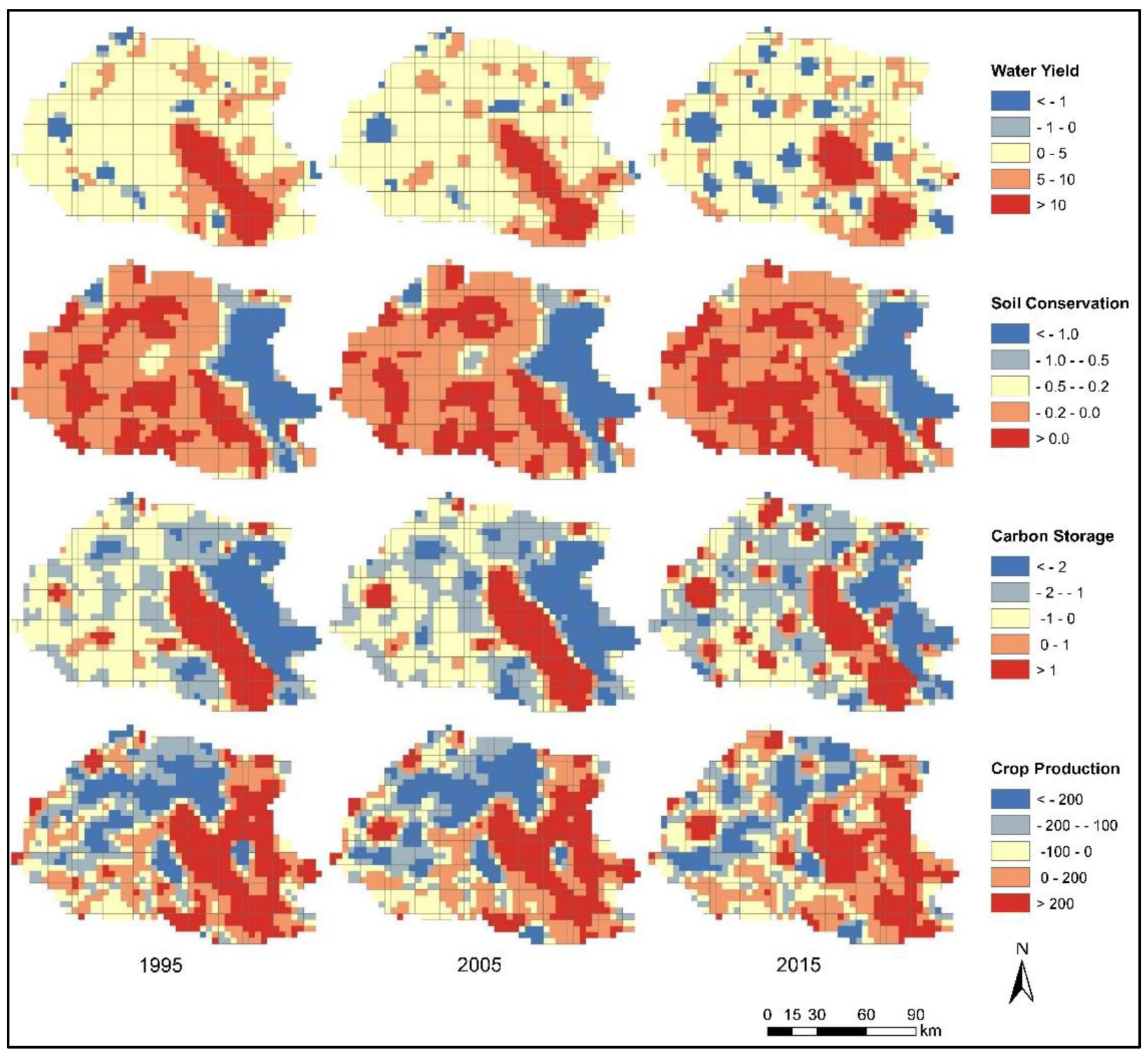
Figure 7 shows the effects of ED on ecosystem services. A stronger positive impact of ED on carbon storage was observed in the city core, while negative and weaker effects were found in the rural areas. This result implies that ED had more significant impact on carbon storage in an urbanized area than in a rural area. The correlation between ED and soil conservation exhibited a relatively high R² value. ED significantly influenced soil conservation, and the impact of ED on soil conservation varied spatiotemporally.

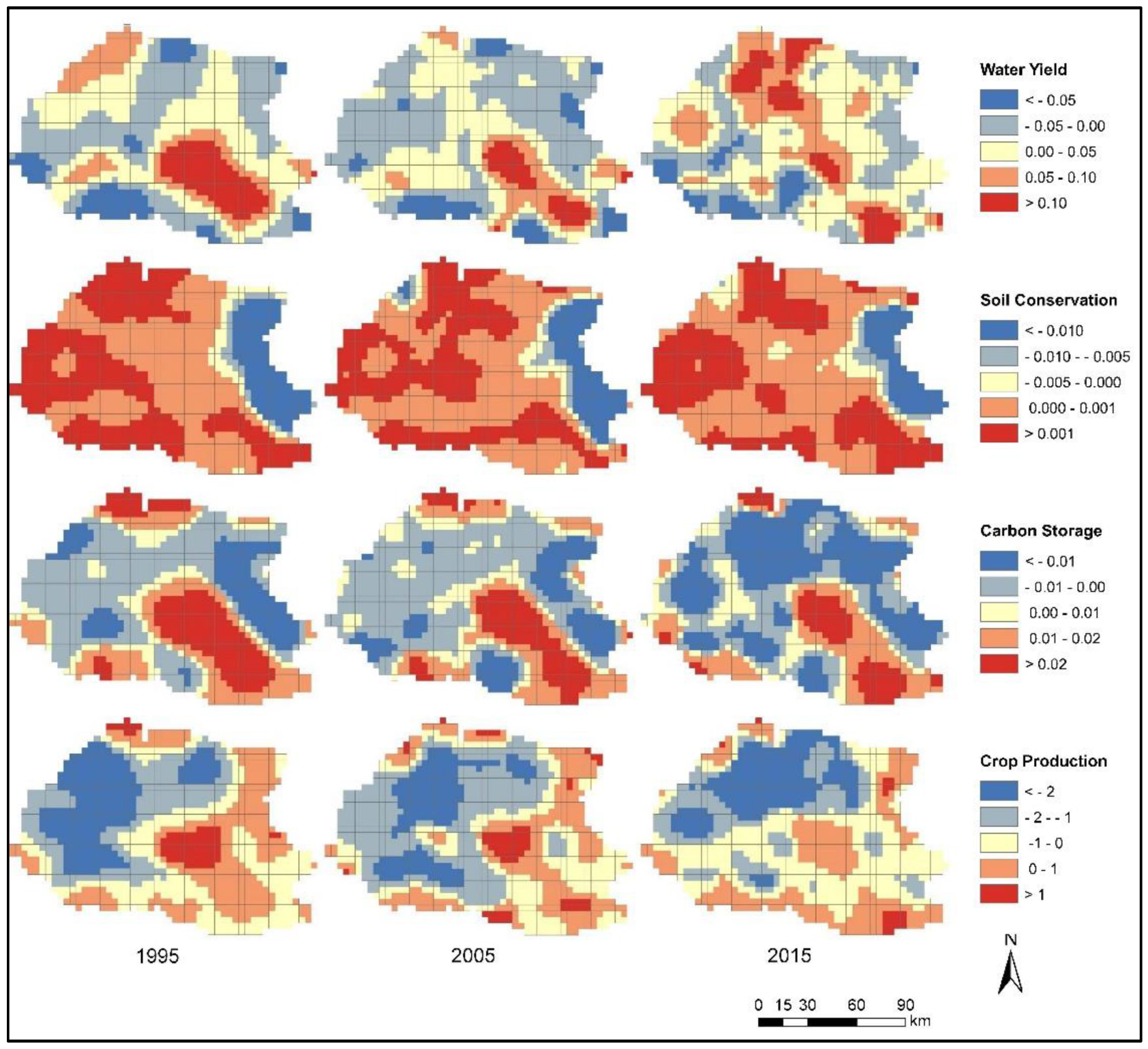
Figure 8 presents maps of the coefficients from the GWR model for the relationship between SHAPE_MN and ecosystem services. SHAPE_MN had a significant negative correlation with crop production in most of the NLB, which suggests that higher crop production is related to a lower SHAPE_MN value. A negative correlation between SHAPE_MN and carbon storage was observed in most of the study area and correlation varied spatiotemporally. In summary, more than 50% of the spatial variation in ecosystem services could be explained by SHAPE_MN.

4. Discussion

4.1. Impacts of Urban Spatial Patterns on Ecosystem Services

Previous urban planning strategies in China only focused on land management in urban construction and farmland protection, and ignored sustainable ecosystem management. Without considering the ecological effects of urban spatial pattern changes, much agricultural land was transformed into built-up land in rapid development areas. Currently, emphasis of land use planning has changed from farmland protection to ecosystem management. Against this background, quantifying ecosystem services and their relationship with related factors is becoming more crucial and practical. This study describes a method to investigate the relationship between urban spatial patterns and ecosystem services during a dramatic urbanization process. Many studies have demonstrated that urbanization causes a reduction in ecosystem services [3,35]. Our findings suggest that ecosystem services decreased in response to urbanization. This outcome is consistent with findings described in other studies that also concluded that urbanization and ecosystem services are significantly correlated. For example, Zhang et al. (2018) highlighted that growth in population caused substantial reduction in in the supply of ecosystem services associated with the urbanization in Wuhan, China [35]. Sun et al. (2018) suggested that the transformation from vegetation land into built-up land is an important factor in the decline of ecosystem services for the Atlanta metropolitan area, United States [36]. Urbanization causes the expansion of built-up land, making the spatial pattern more irregular and fragmented [33]. Unlike socioeconomic variables (e.g., GDP and population) and land use structure indicators used in previous studies, we analyzed the effect of urban spatial patterns on ecosystem services.

Moreover, results revealed by the GWR model show that the changes in the supply of the ecosystem services evaluated in the NLB could be explained by urbanization induced spatial pattern changes with a relatively high goodness of fit. Therefore, optimizing urban spatial patterns is regarded as another effective way to realize sustainable ecosystem development besides limiting urban expansion. By considering the actual local situation, and the spatiotemporally varying impact of urban spatial patterns, it is possible to develop appropriate ecosystem management measures and development policies to avoid the negative effects of urban spatial pattern changes on ecosystem services as well as to promote regional sustainable development.

4.2. Methodological Implication

Selecting a suitable model is of substantial importance for revealing the relationship between urban spatial patterns and ecosystem services. Numerous studies have explored the global relationship by using traditional regression models [37,38]. Our research extended these efforts by examining the spatiotemporally varying impacts of urban spatial patterns rather than the global average impact. The OLS model analyzes the study area as a whole and reveals a global average relationship. In contrast, the use of the GWR model enables spatial variability of results to be presented and analyzed. This approach facilitated more precise identification of urban spatial pattern impact on ecosystem services change in the NLB. The GWR model enabled the analysis of each variable’s behavior at the local level revealing the spatial variability among them. Detailed information on the varying impacts of urban spatial patterns on ecosystem services for different locations of the study area was revealed by the GWR model. This approach can be useful to develop more suitable and effective planning policies to avoid the negative ecological effects of variation in urban spatial patterns according to the local situation. In addition, the temporally varying impact of urban spatial patterns on ecosystem services has been neglected in traditional analyses. To fill this research gap, the temporal dimension was incorporated into this study. The results enabled us to analyze how the relationships temporally change along with the urbanization process.

4.3. Outlook

It has been widely accepted in previous studies that the spatial scale is a crucial problem in geography and ecology research [39]. Both the landscape pattern and ecosystem services values are scale dependent. A different grid size could result in a different relationship between independent and dependent variables. Although a preliminary test was carried out in this study to choose the optimal grid size, the scale effect of spatial patterns on ecosystem services should be fully investigated by comparing different grid sizes. Additionally, only four ecosystem services were considered in this study due to difficulties in data acquisition. These four services could only reveal part of the changes. Ecosystem services are more complex than the services selected in this investigation. Including more ecosystem service types in future studies could provide more comprehensive information.

5. Conclusions

Scientifically examining the relationships between urban spatial patterns and ecosystem services is important for effective urban planning and sustainable development. The NLB experienced rapid urbanization between 1995 and 2015, which not only resulted in significant change in urban spatial patterns, but also affected ecosystem services in numerous ways. Therefore, we sought to explain to what extent the urban spatial patterns induced by urbanization are related to changes in ecosystem services in the NLB by using remote sensing, spatial pattern analysis, and the GWR model. Urban spatial patterns were quantified using four spatial metrics: PLAND, PD, ED, and SHAPE_MN, with ecosystem services being represented by water yield, soil conservation, carbon storage and crop production.

We found that water yield, soil conservation, carbon storage and crop production in the NLB declined by 9.70%, 4.01%, 7.51%, and 9.67%, respectively, during urbanization in the period of 1995–2015. Both urban spatial patterns and ecosystem services exhibited obvious spatial variability. The areas showing the highest deterioration in the selected ecosystem services were mainly found in the city core, which corresponds to urban growth. Moreover, urban spatial patterns and ecosystem services were significantly correlated, which indicates that urban spatial patterns can significantly affect ecosystem services. More importantly, the GWR model revealed the spatial nonstationary relationship between urban spatial patterns and ecosystem services.

In addition, the GWR model was demonstrated to be more effective in examining the relationships between ecosystem services and urban spatial patterns than the OLS model, as evidenced by the larger adjusted R², smaller AICc and absolute Moran’s I value. Moreover, the estimated parameters generated by the GWR model indicate that the impact of urban spatial patterns on ecosystem services varies spatiotemporally. Therefore, to realize sustainable development in the NLB, there is a need to develop effective policies for different locations and different phases of the urbanization process.