An Automatic Method for Detection and Update of Additive Changes in Road Network with GPS Trajectory Data


Abstract
:1. Introduction
2. Related Work
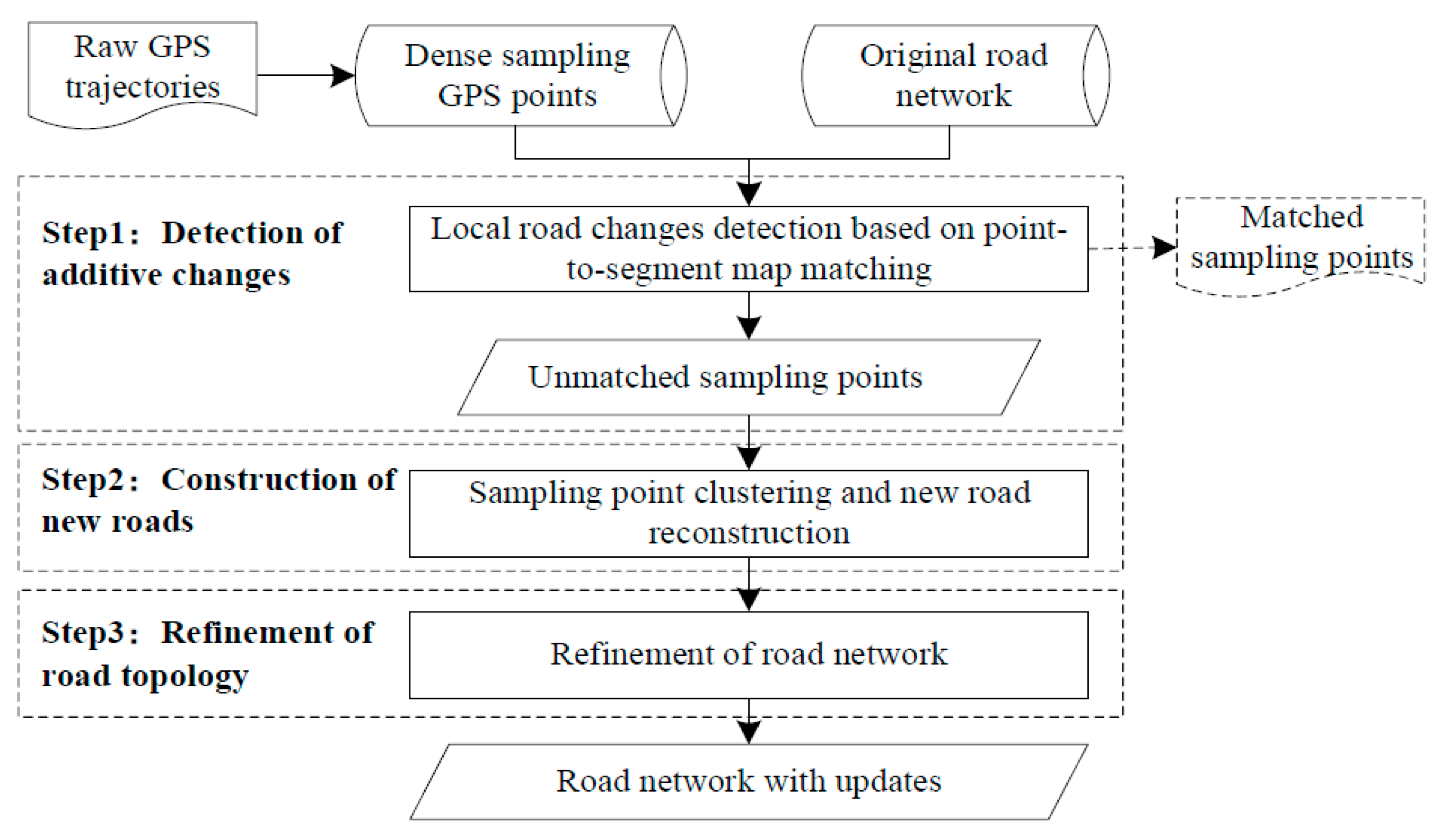
3. Methodology
3.1. Data Preprocessing
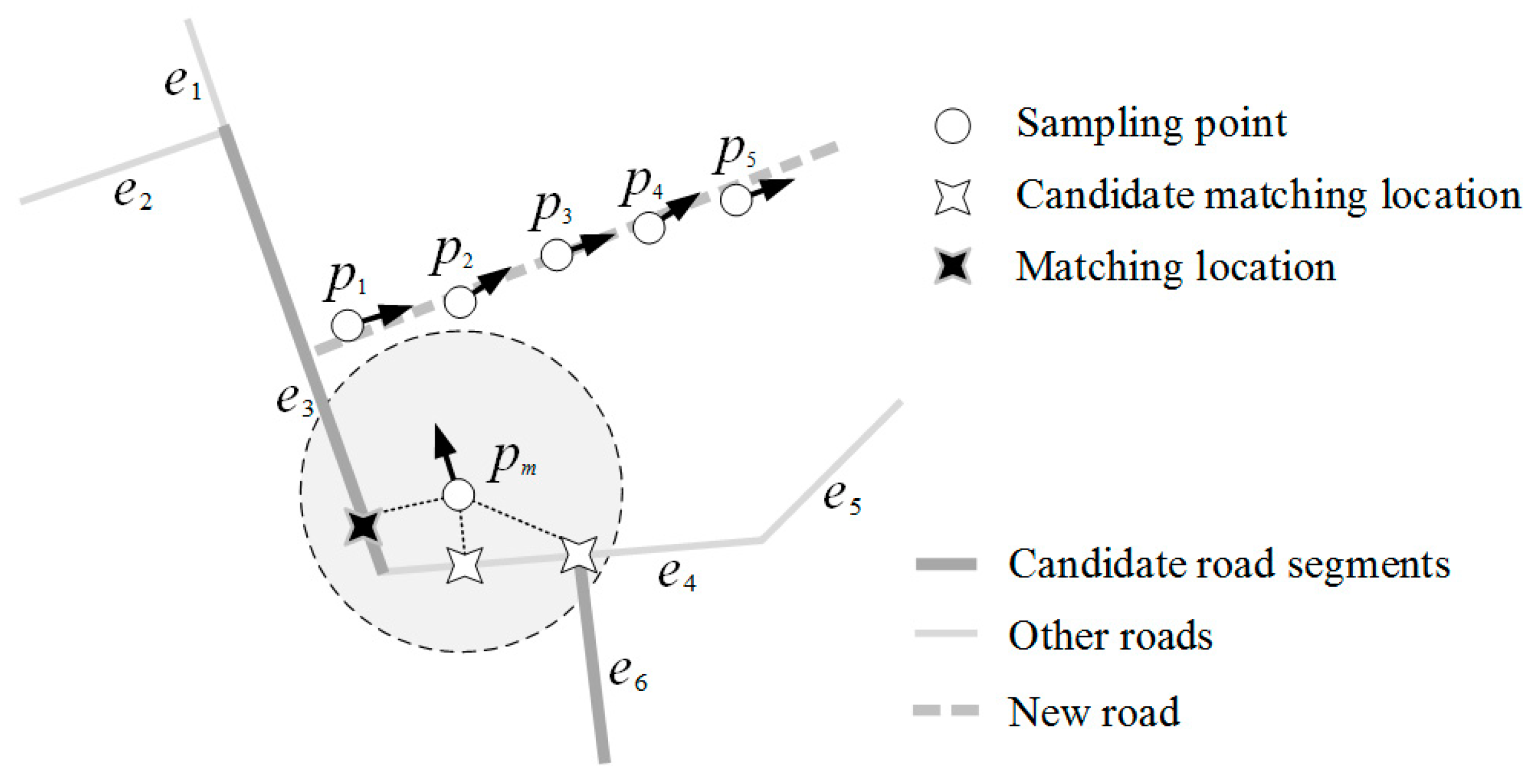
3.2. Detection of Additive Changes
- (a)
- First, the spatial distances from the sampling point to all the road segments are computed, and road segments are filtered if the distances between the road segments and the sampling point are larger than a distance threshold; e.g., 50 meters.
- (b)
- Second, for the remaining road segments, a road segment is recognized as a candidate road segment if the angle between the heading direction of the sampling point and the direction of the road segment is smaller than an angle threshold; e.g., 15 degrees.
- (c)
- In all the candidate road segments, the road segment with the smallest spatial distance to the sampling point is finally recognized as the road segment matching the sampling point. If there is not a road segment matching the sampling point, the sampling point is recognized as an unmatched sampling point.
3.3. Construction of New Roads: A Decomposition-Combination Map Generation Algorithm
3.3.1. Decomposition of Complex New Roads
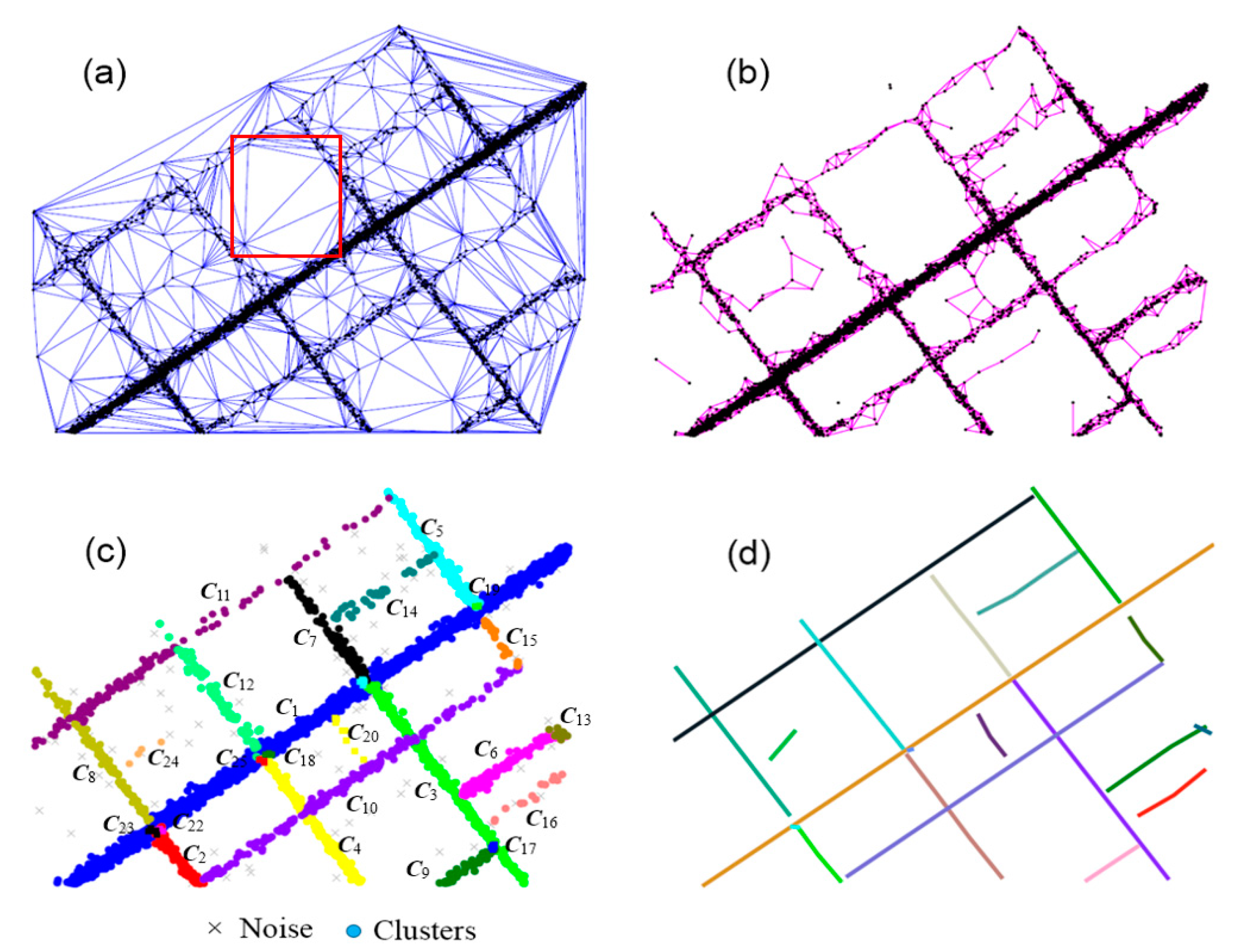
3.3.2. Road Centerline Extraction
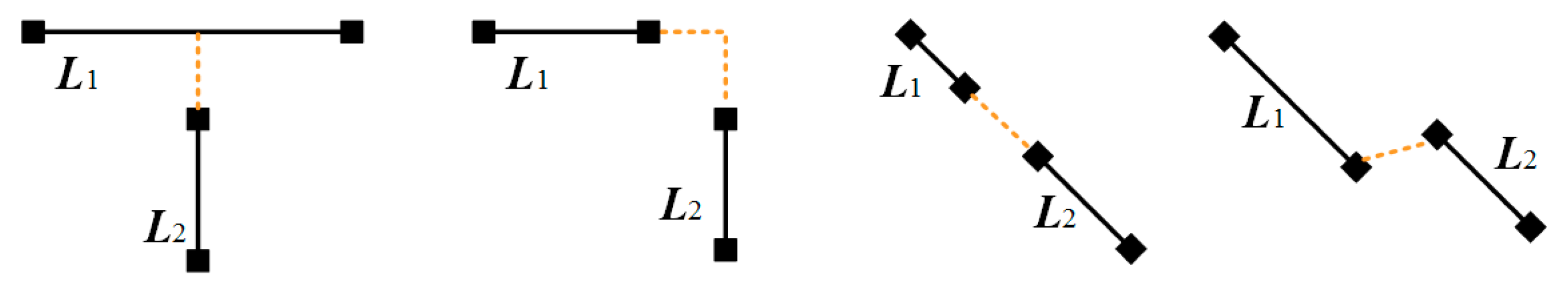
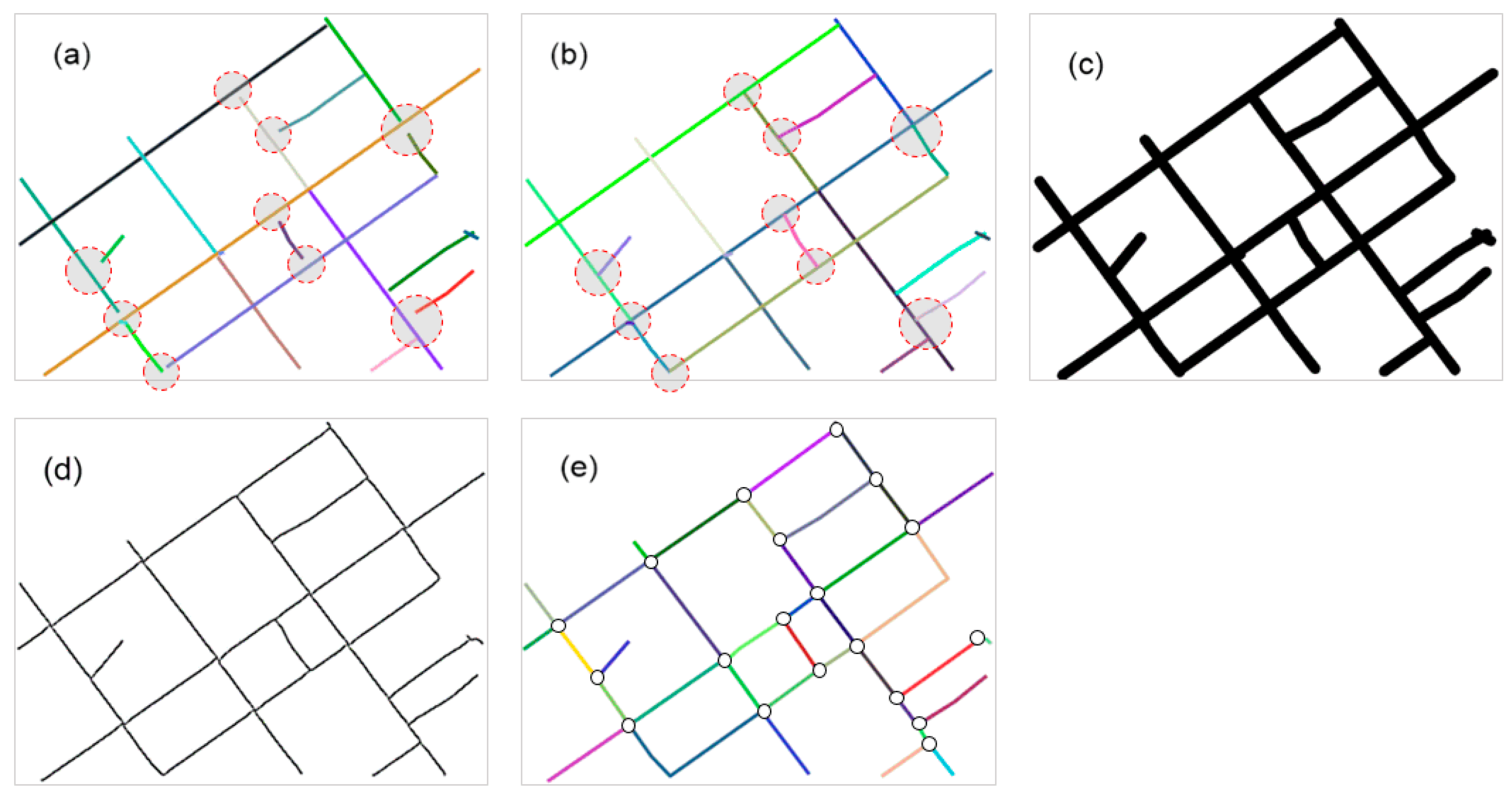
3.4. Topology Refinement of the Road Network
- (a)
- First, each road segment (or road curve) is virtually extended outward at both the beginning and ending points along the direction of the road (specially, along the direction of the line segments where the beginning and ending points are on). We then check if the extended road segments (or curves) are intersected with each. If a road segment intersects with others, then this road segment is extended to its nearest intersecting road segment, as the roads in red circles shown in Figure 5b. The extension distance is set to 30 m in this paper, according to GPS positioning errors.
- (b)
- Then, the buffer zones of the above road segments are created and converted into a binary image as shown in Figure 5c. It can be seen that the gaps between the road segments that should be connected are filled. The buffer size is set to 20 m according to the road width.
- (c)
- (d)
- Finally, the above-generated road skeleton centerlines are divided into different road segments at the junction points (see Figure 5e). The junction points are detected by checking whether this point connects three or more road segments. The Douglas–Peucker algorithm [39] is further applied to remove the unnecessary intermediate points in the road segments, and the distance parameter for the Douglas–Peucker algorithm is set to 3 m in our experiments. The allowable transitions between two road segments are determined according to whether there exists at least one trajectory matching both these two road segments. Figure 5e shows the refined road network.
4. Experimental Results
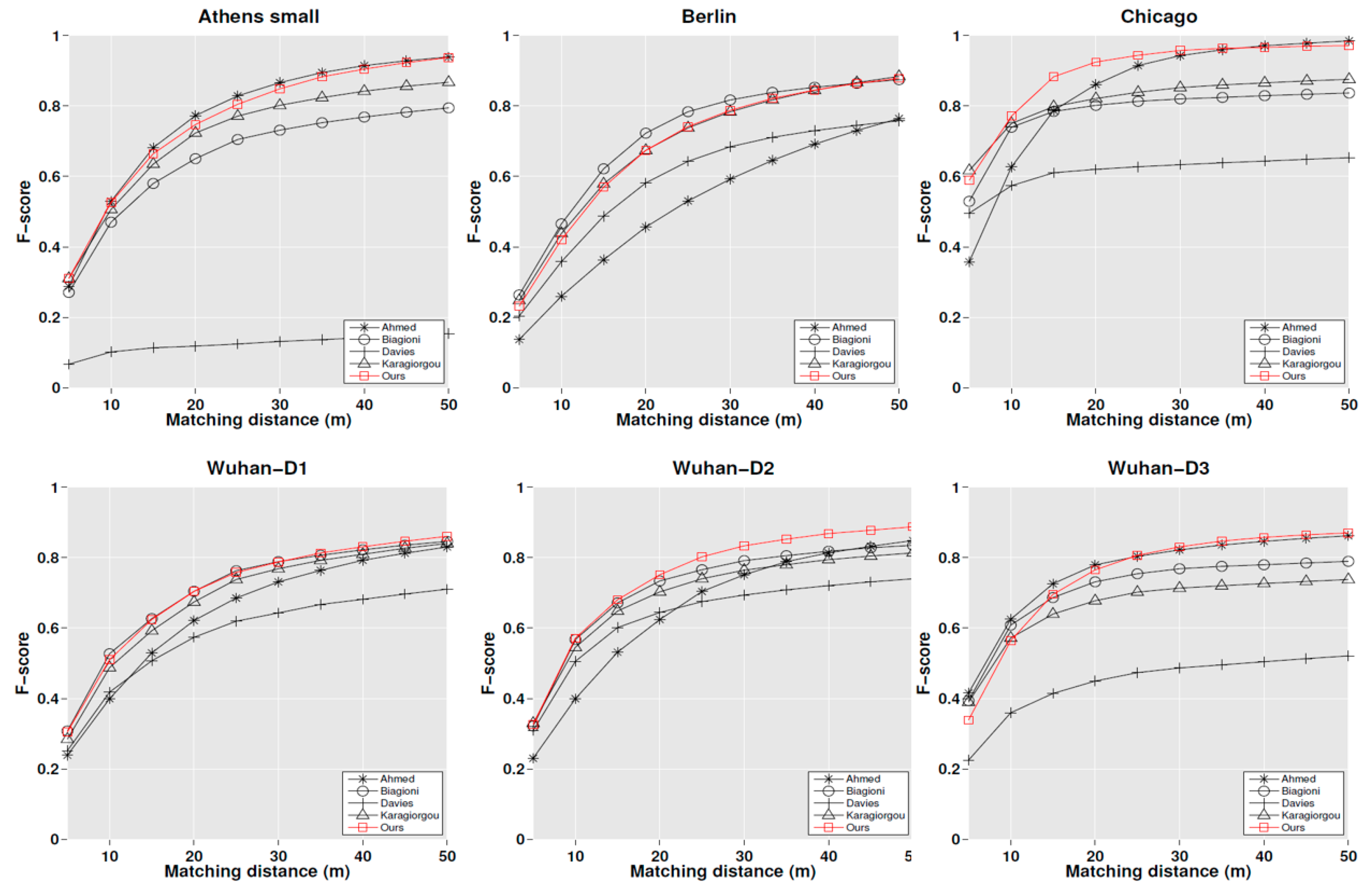
4.1. Experiment I: Performance on the Construction of New Roads
4.1.1. Time Complexity
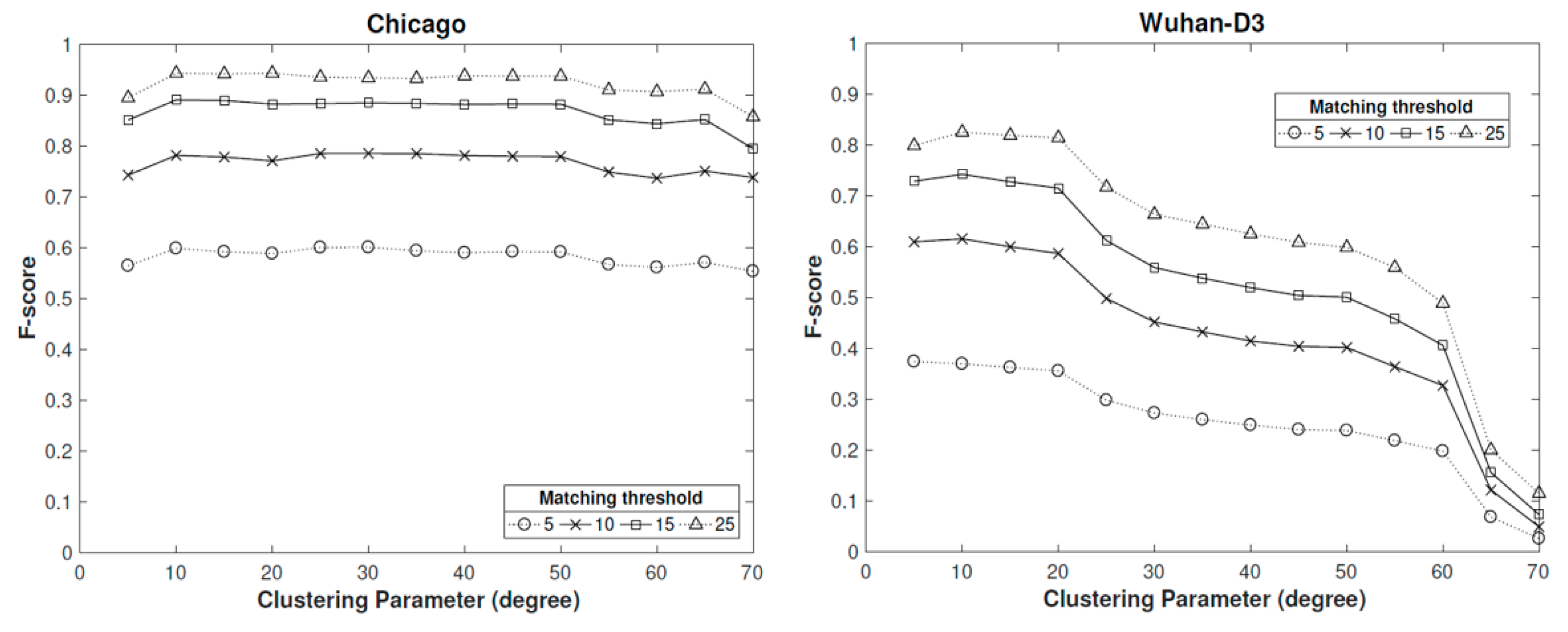
4.1.2. Parameter Sensitivity
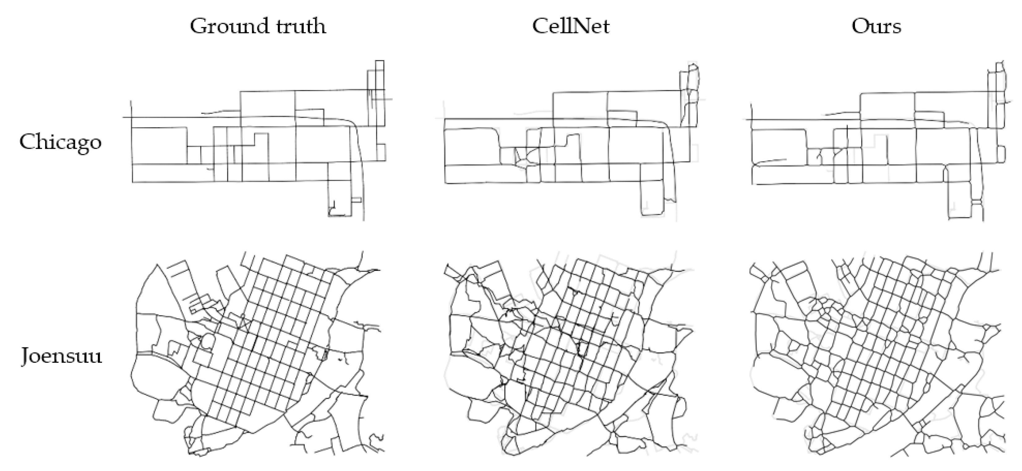
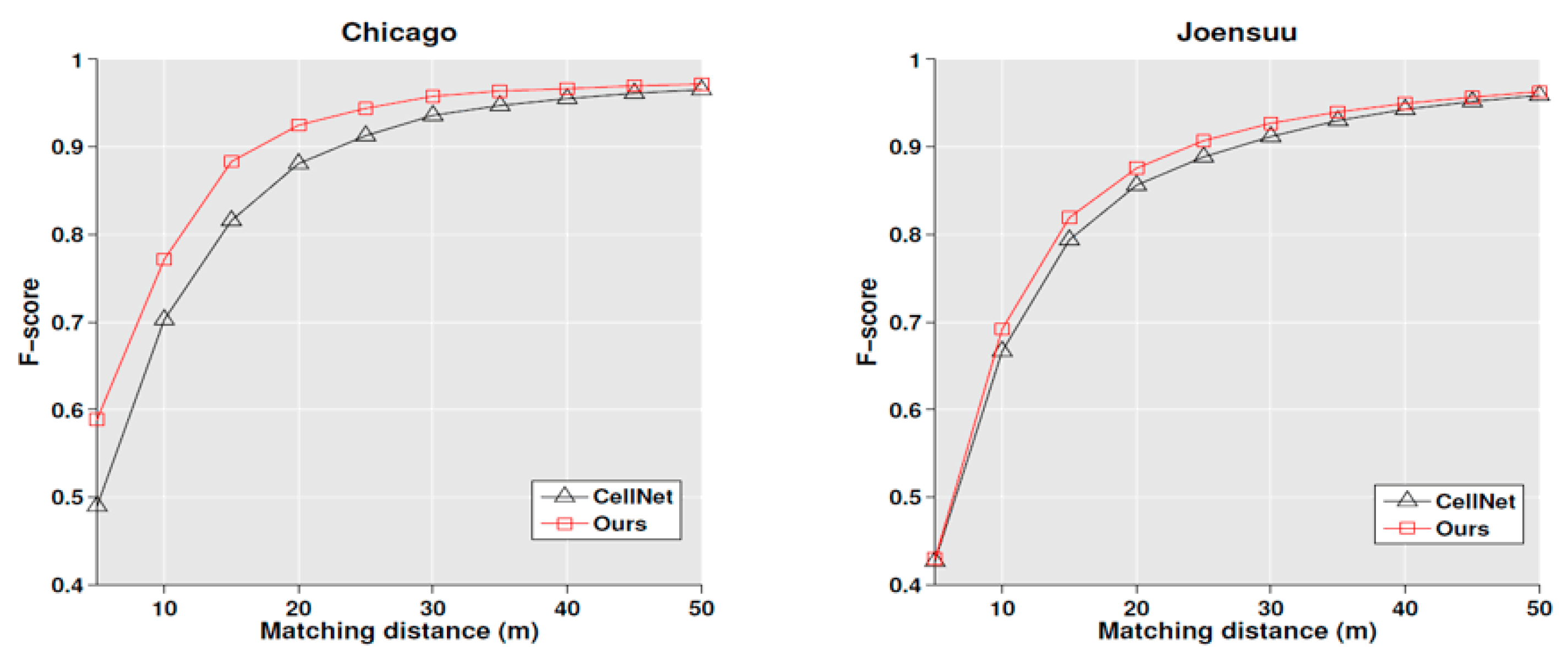
4.2. Experiment II: Application of the Proposed Method for the Update of the Road Network
5. Conclusions
Author Contributions
Acknowledgments
Conflicts of Interest
References
- Zhang, Y.C.; Liu, J.P.; Qian, X.L.; Qiu, A.G.; Zhang, F.H. An automatic road network construction method using massive gps trajectory data. ISPRS Int. J. Geo Inf. 2017, 6, 400. [Google Scholar] [CrossRef]
- Tang, L.L.; Ren, C.; Liu, Z.; Li, Q.Q. A road map refinement method using Delaunay triangulation for big trace data. ISPRS Int. J. Geo Inf. 2017, 6, 45. [Google Scholar] [CrossRef]
- Edelkamp, S.; Schrodl, S. Route planning and map inference with global positioning traces. In Computer Science in Perspective; Springer: New York, NY, USA, 2003; Volume 2598, pp. 128–151. [Google Scholar]
- Davies, J.J.; Beresford, A.R.; Hopper, A. Scalable, distributed, real-time map generation. IEEE Pervas. Comput. 2006, 5, 47–54. [Google Scholar] [CrossRef]
- Cao, L.; Krumm, J. From GPS traces to a routable road map. ACM SIGSPATIAL international conference on advances in geographic information systems. In Proceedings of the 17th ACM SIGSPATIAL International Conference on Advances in Geographic Information Systems, Seattle, WA, USA, 4–6 November 2009; pp. 3–12. [Google Scholar]
- Ahmed, M.; Wenk, C. Constructing street networks from GPS trajectories. In Proceedings of the European Symposium on Algorithms, Ljubljana, Slovenia, 10–12 September 2012; pp. 60–71. [Google Scholar]
- Biagioni, J.; Eriksson, J. Map inference in the face of noise and disparity. In Proceedings of the ACM 20th International Conference on Advances in Geographic Information Systems, Redondo Beach, CA, USA, 6–9 November 2012; pp. 79–88. [Google Scholar]
- Karagiorgou, S.; Pfoser, D. On vehicle tracking data-based road network generation. In Proceedings of the ACM 20th International Conference on Advances in Geographic Information Systems, Redondo Beach, CA, USA, 6–9 November 2012; pp. 89–98. [Google Scholar]
- Wang, J.; Rui, X.P.; Song, X.F.; Tan, X.S.; Wang, C.L.; Raghavan, V. A novel approach for generating routable road maps from vehicle GPS traces. Int. J. Geogr. Inf. Sci. 2015, 29, 69–91. [Google Scholar] [CrossRef]
- Mori, U.; Mendiburu, A.; Alvarez, M.; Lozano, J.A. A review of travel time estimation and forecasting for advanced traveller information systems. Transp. A Trans. Sci. 2015, 11, 119–157. [Google Scholar] [CrossRef]
- Yang, X.; Tang, L.L.; Stewart, K.; Dong, Z.; Zhang, X.; Li, Q.Q. Automatic change detection in lane-level road networks using gps trajectories. Int. J. Geogr. Inf. Sci. 2018, 32, 601–621. [Google Scholar] [CrossRef]
- Deng, M.; Huang, J.C.; Zhang, Y.F.; Liu, H.M.; Tang, L.L.; Tang, J.B.; Yang, X.X. Generating urban road intersection models from low-frequency gps trajectory data. Int. J. Geogr. Inf. Sci. 2018, 32, 2337–2361. [Google Scholar] [CrossRef]
- Wang, W.; Jin, J.; Ran, B.; Guo, X.C. Large-scale freeway network traffic monitoring: A map-matching algorithm based on low-logging frequency GPS probe data. J. Intell. Transp. Syst. 2011, 15, 63–74. [Google Scholar] [CrossRef]
- Huang, J.C.; Deng, M.; Tang, J.B.; Hu, S.L.; Liu, H.M.; Wariyo, S.; He, J.Q. Automatic generation of road maps from low quality GPS trajectory data via structure learning. IEEE Access 2018, 6, 71965–71975. [Google Scholar] [CrossRef]
- Schroedl, S.; Wagstaff, K.; Rogers, S.; Langley, P.; Wilson, C. Mining GPS traces for map refinement. Data Min. Knowl. Disc. 2004, 9, 59–87. [Google Scholar] [CrossRef]
- Ahmed, M.; Karagiorgou, S.; Pfoser, D.; Wenk, C. A comparison and evaluation of map construction algorithms using vehicle tracking data. Geoinformatica 2015, 19, 601–632. [Google Scholar] [CrossRef]
- Chen, C.; Cheng, Y.H. Roads digital map generation with multi-track GPS data. In Proceedings of the International Workshop on Geoscience and Remote Sensing, Shangai, China, 21–22 December 2008; pp. 508–511. [Google Scholar]
- Shi, W.H.; Shen, S.H.; Liu, Y.C. Automatic generation of road network map from massive GPS vehicle trajectories. In Proceedings of the 12th International IEEE Conference on Intelligent Transportation Systems (ITSC 2009), St. Louis, MO, USA, 4–7 October 2009; pp. 48–53. [Google Scholar]
- Wang, S.Y.; Wang, Y.S.; Li, Y.J. Efficient map reconstruction and augmentation via topological methods. In Proceedings of the 23rd ACM International Conference on Advances in Geographic Information Systems, Seattle, WA, USA, 3–6 November 2015. [Google Scholar]
- Worrall, S.; Nebot, E. Automated process for generating digitised maps through GPS data compression. In Australasian Conference on Robotics and Automation; ACRA: Brisbane, Australia, 2007; Volume 6. [Google Scholar]
- Agamennoni, G.; Nieto, J.I.; Nebot, E.M. Robust inference of principal road paths for intelligent transportation systems. IEEE Trans. Intell. Transp. Syst. 2011, 12, 298–308. [Google Scholar] [CrossRef]
- Kuntzsch, C.; Sester, M.; Brenner, C. Generative models for road network reconstruction. Int. J. Geogr. Inf. Sci. 2016, 30, 1012–1039. [Google Scholar] [CrossRef]
- Mariescu-Istodor, R.; Fränti, P. CellNet: Inferring road networks from GPS trajectories. ACM Trans. Spat. Algorithms Syst. 2018, 4, 1–22. [Google Scholar] [CrossRef]
- Wu, T.; Xiang, L.G.; Gong, J.Y. Updating road networks by local renewal from gps trajectories. ISPRS Int. J. Geo Inf. 2016, 5, 163. [Google Scholar] [CrossRef]
- Zhao, Y.; Liu, J.; Chen, R.Q.; Li, J.; Xie, C.; Niu, W.J.; Geng, D.Y.; Qin, Q.M. A new method of road network updating based on floating car data. In Proceedings of the 2011 IEEE International Geoscience and Remote Sensing Symposium, Vancouver, BC, Canada, 24–29 July 2011; pp. 1878–1881. [Google Scholar]
- Fang, W.; Hu, R.; Xu, X.; Xia, Y.; Hung, M.H. A novel road network change detection algorithm based on floating car tracking data. In Telecommunication Systems; Springer: New York, NY, USA, 2016; pp. 1–7. [Google Scholar]
- Tang, L.L.; Huang, F.; Zhang, X.; Xu, H. Road network change detection based on floating car data. J. Netw. 2012, 7, 1063–1070. [Google Scholar] [CrossRef]
- Wang, Y.; Liu, X.; Wei, H.; Forman, G.; Chen, C.; Zhu, Y. CrowdAtlas: Self-updating maps for cloud and personal use. In Proceedings of the ACM International Conference on Mobile Systems, Taipei, Taiwan, 25–28 June 2013; pp. 27–40. [Google Scholar]
- Shan, Z.Q.; Wu, H.; Sun, W.W.; Zheng, B.H. Cobweb: A robust map update system using GPS trajectories. In Proceedings of the 2015 ACM International Joint Conference on Pervasive and Ubiquitous Computing (Ubicomp 2015), Osaka, Japan, 7–11 September 2015; pp. 927–937. [Google Scholar]
- Brakatsoulas, S.; Pfoser, D.; Salas, R.; Wenk, C. On map-matching vehicle tracking data. In Proceedings of the 31st International Conference on Very Large Databases, Trondheim, Norway, 30 August–2 September 2005; pp. 853–864. [Google Scholar]
- Newson, P.; Krumm, J. Hidden Markov map matching through noise and sparseness. In Proceedings of the 17th ACM SIGSPATIAL International Conference on Advances in Geographic Information Systems—GIS, Seattle, WA, USA, 4–6 November 2009. [Google Scholar]
- Chen, B.Y.; Yuan, H.; Li, Q.Q.; Lam, W.H.K.; Shaw, S.L.; Yan, K. Map-matching algorithm for large-scale low-frequency floating car data. Int. J. Geogr. Inf. Sci. 2014, 28, 22–38. [Google Scholar] [CrossRef]
- Li, Z.; Yan, H.; Ai, T.; Chen, J. Automated building generalization based on urban morphology and gestalt theory. Int. J. Geogr. Inf. Sci. 2004, 18, 513–534. [Google Scholar] [CrossRef]
- Deng, M.; Tang, J.B.; Liu, Q.L.; Wu, F. Recognizing building groups for generalization: A comparative study. Cartogr. Geogr. Inf. Sci. 2018, 45, 187–204. [Google Scholar] [CrossRef]
- Ester, M.; Kriegel, H.-P.; Sander, J.; Xu, X. A Density-Based Algorithm for Discovering Clusters in Large Spatial Databases with Noise; Institute for Computer Science, University of Munich: Munich, Germany, 1996; pp. 226–231. [Google Scholar]
- Deng, M.; Liu, Q.L.; Cheng, T.; Shi, Y. An adaptive spatial clustering algorithm based on Delaunay triangulation. Comput. Environ. Urban. 2011, 35, 320–332. [Google Scholar] [CrossRef]
- Pittman, J.; Murthy, C.A. Fitting optimal piecewise linear functions using genetic algorithms. IEEE Trans. Pattern Anal. 2000, 22, 701–718. [Google Scholar] [CrossRef]
- Lam, L.; Lee, S.W.; Suen, C.Y. Thinning methodologies—A comprehensive survey. In IEEE Transactions on Pattern Analysis and Machine Intelligence; IEEE Compute Society: Washington, DC, USA, 1992; Volume 14, pp. 869–885. [Google Scholar] [CrossRef]
- Douglas, D.; Peucker, T. Algorithms for the reduction of the number of points required to represent a digitized line or its caricature. Can. Cartograph. 1973, 10, 112–122. [Google Scholar] [CrossRef]


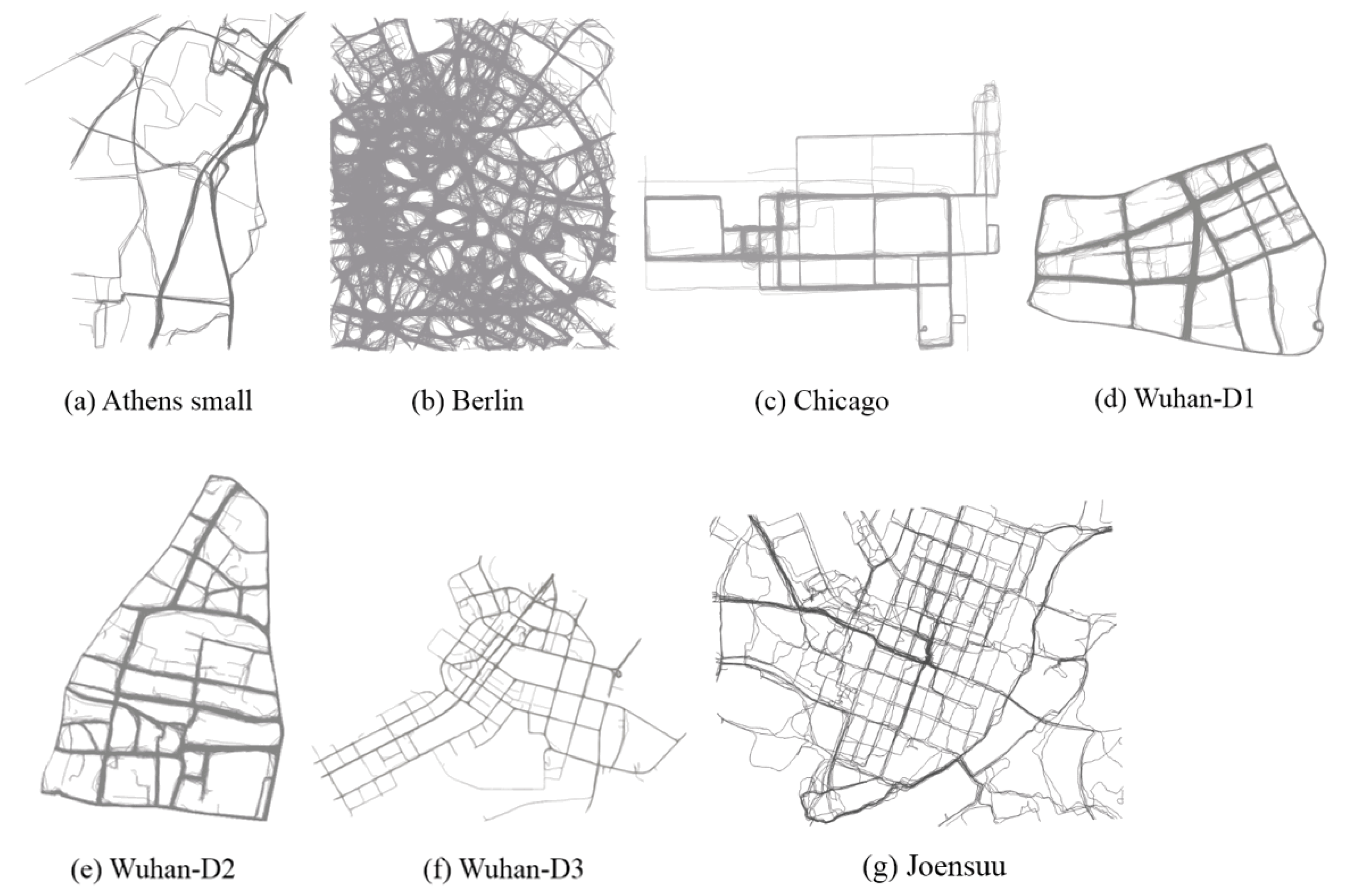
| ID | Dataset | Country | Number of Trajectories | Average Sampling Rate (s) | Trajectory Length (km) |
|---|---|---|---|---|---|
| 1 | Athens small | Greece | 129 | 34.07 | 443 |
| 2 | Berlin | Germany | 26,831 | 41.98 | 41,116 |
| 3 | Chicago | USA | 889 | 3.61 | 2869 |
| 4 | Wuhan-D1 | China | 5843 | 49.24 | 4107 |
| 5 | Wuhan-D2 | China | 9584 | 49.24 | 5471 |
| 6 | Wuhan-D3 | China | 2706 | 49.24 | 3253 |
| 7 | Joensuu | Finland | 108 | 2.00 | 250 |
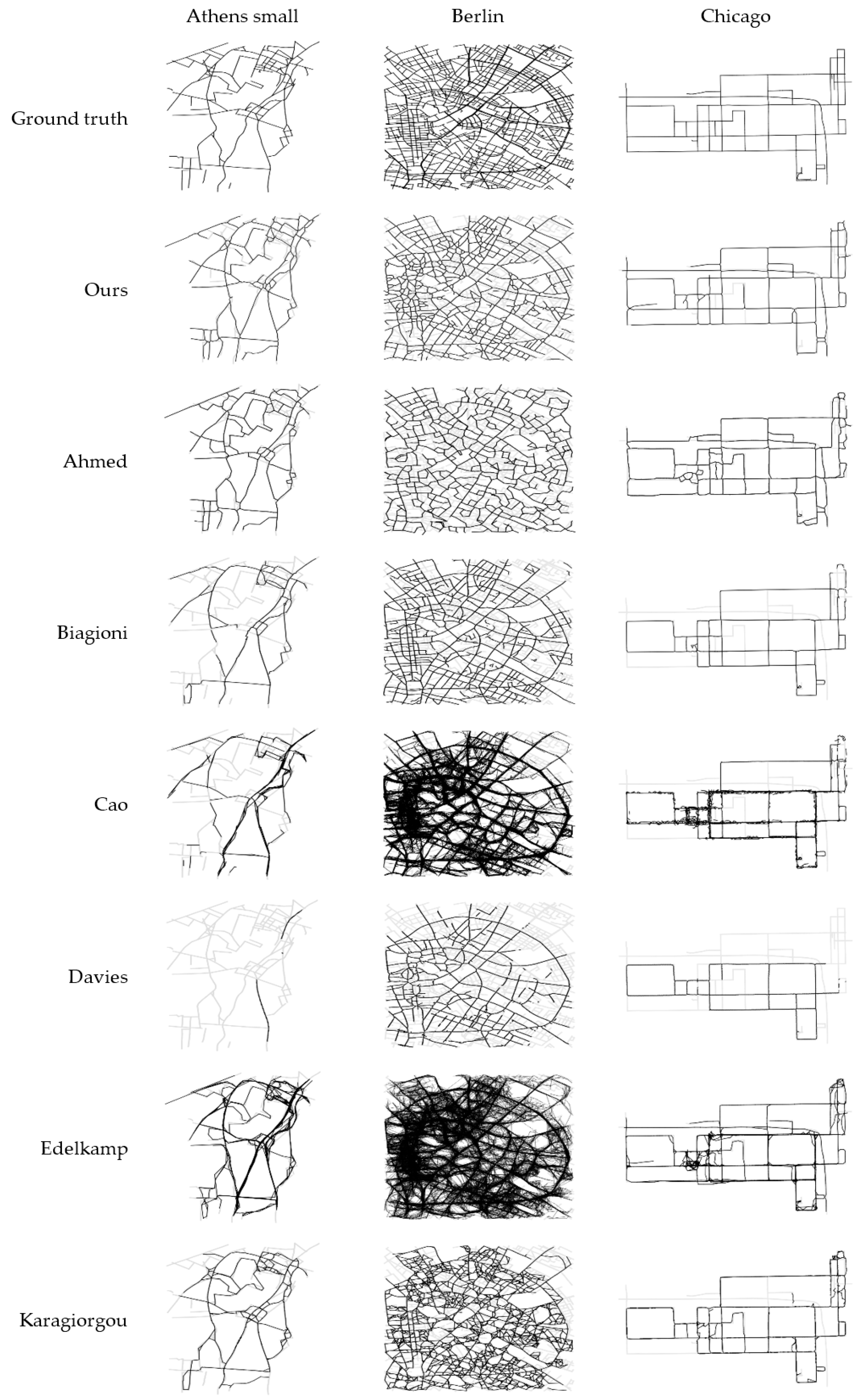
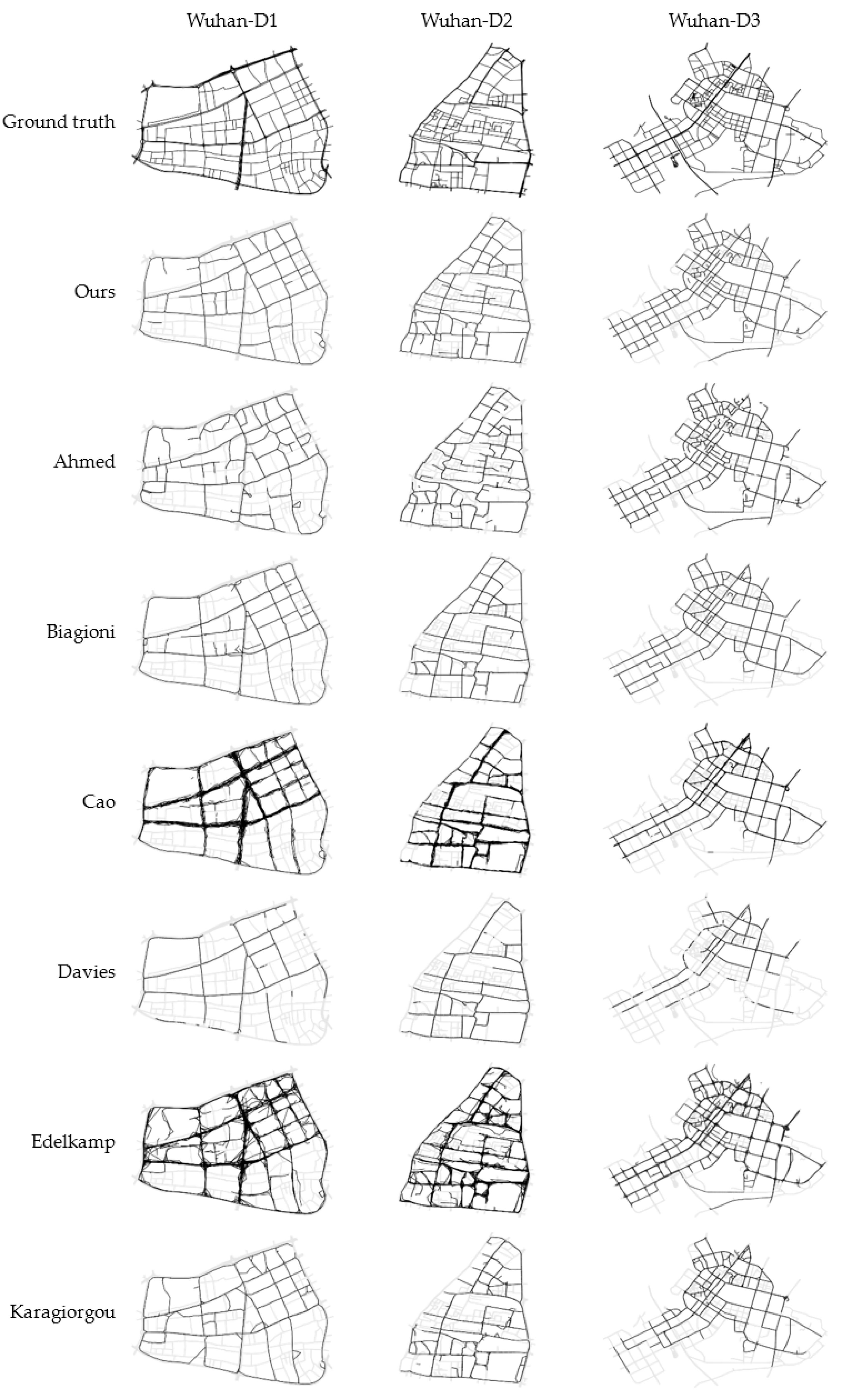
| Number | Source | Method |
|---|---|---|
| 1 | Edelkamp & Schrödl (2003) | Point clustering |
| 2 | Davies et al. (2006) | Density image skeleton extraction |
| 3 | Cao & Krumm (2009) | Incremental track insertion |
| 4 | Biagioni & Eriksson (2012) | Density image skeleton extraction |
| 5 | Ahmed & Wenk (2012) | Incremental track insertion |
| 6 | Karagiorgou & Pfoser (2012) | Intersection linking |
| 7 | Mariescu-Istodor & Fränti (2018) | Intersection linking |
| Dataset | Ahmed (Java) | Biagioni (Python) | Cao (Python) | Davies (Python) | Edelkamap (Python) | Karagiorgou (MATLAB) | Ours (Octave) |
|---|---|---|---|---|---|---|---|
| Athens small | 0.087 | 16.19 | 4.73 | 0.41 | 1.47 | 6.95 | 0.56 |
| Berlin | 82.54 | 301.70 | 727.96 | 108.77 | >20 h | >48 h | 13.14 |
| Chicago | 23.67 | 31.25 | 373.01 | 1.68 | 18.49 | >20 h | 3.64 |
| Wuhan-D1 | 6.15 | 54.40 | 127.48 | 4.86 | 42.44 | 426.44 | 3.57 |
| Wuhan-D2 | 13.48 | 44.21 | 162.43 | 10.67 | 84.64 | 451.28 | 4.06 |
| Wuhan-D3 | 10.65 | 20.78 | 21.93 | 9.38 | 53.46 | 85.67 | 1.51 |
© 2019 by the authors. Licensee MDPI, Basel, Switzerland. This article is an open access article distributed under the terms and conditions of the Creative Commons Attribution (CC BY) license (http://creativecommons.org/licenses/by/4.0/).
Share and Cite
Tang, J.; Deng, M.; Huang, J.; Liu, H.; Chen, X. An Automatic Method for Detection and Update of Additive Changes in Road Network with GPS Trajectory Data. ISPRS Int. J. Geo-Inf. 2019, 8, 411. https://0-doi-org.brum.beds.ac.uk/10.3390/ijgi8090411
Tang J, Deng M, Huang J, Liu H, Chen X. An Automatic Method for Detection and Update of Additive Changes in Road Network with GPS Trajectory Data. ISPRS International Journal of Geo-Information. 2019; 8(9):411. https://0-doi-org.brum.beds.ac.uk/10.3390/ijgi8090411
Chicago/Turabian StyleTang, Jianbo, Min Deng, Jincai Huang, Huimin Liu, and Xueying Chen. 2019. "An Automatic Method for Detection and Update of Additive Changes in Road Network with GPS Trajectory Data" ISPRS International Journal of Geo-Information 8, no. 9: 411. https://0-doi-org.brum.beds.ac.uk/10.3390/ijgi8090411