Generation of Lane-Level Road Networks Based on a Trajectory-Similarity-Join Pruning Strategy


1
State Key Laboratory of Information Engineering in Surveying, Mapping, and Remote Sensing, Wuhan University, Wuhan 430079, China
2
Engineering Research Center for Spatio-Temporal Data Smart Acquisition and Application, Ministry of Education of China, Wuhan 430079, China
3
Three Gorges Geotechnical Consultants Co., Ltd., Wuhan 430074, China
*
Author to whom correspondence should be addressed.
ISPRS Int. J. Geo-Inf. 2019, 8(9), 416; https://0-doi-org.brum.beds.ac.uk/10.3390/ijgi8090416
Submission received: 3 June 2019
/
Revised: 4 September 2019
/
Accepted: 8 September 2019
/
Published: 16 September 2019
(This article belongs to the Special Issue Artificial Intelligence Solutions for Geospatial Analysis: An Integrated Approach)
Abstract
:With the development of autonomous driving, lane-level maps have attracted significant attention. Since the lane-level road network is an important part of the lane-level map, the efficient, low-cost, and automatic generation of lane-level road networks has become increasingly important. We propose a new method here that generates lane-level road networks using only position information based on an autonomous vehicle and the existing lane-level road networks from the existing road-level professionally surveyed without lane details. This method uses the parallel relationship between the centerline of a lane and the centerline of the corresponding segment. Since the direct point-by-point computation is huge, we propose a method based on a trajectory-similarity-join pruning strategy (TSJ-PS). This method uses a filter-and-verify search framework. First, it performs quick segmentation based on the minimum distance and then uses the similarity of two trajectories to prune the trajectory similarity join. Next, it calculates the centerline trajectory for lanes using the simulation transformation model by the unpruned trajectory points. Finally, we demonstrate the efficiency of the algorithm and generate a lane-level road network via experiments on a real road.
1. Introduction
Intelligent driving technology is developing rapidly in both industry and academia. Digital maps can help with advanced driver-assistance systems and autonomous driving. For example, driving applications such as positioning [1,2], driving path planning [3], and decision-making [4] benefit from the auxiliary information in digital maps. Digital maps are used to provide the surrounding information of a vehicle, which facilitates perception applications [5,6] for intelligent driving systems.
An electronic navigation map is a road-level map, used mainly by drivers, that provides basic road navigation functions based on a common map. Due to a lack of lane details, existing electronic navigation maps are not widely used in the development of autonomous driving functions. Thus, research interest has been increasing in lane-level maps with precise lane-level details. In China, 19 companies have conducted investigations in lane-level mapping since 2019. Compared with road-level maps, lane-level maps contain rich lane data [7], with accuracy ranging from a few meters to the decimeter or even centimeter level under various autonomous vehicle functions [8]. The road network is an important aspect of maps and plays an important role in intelligent driving projects [9]. As a key enabling technology, the generation of lane-level road networks is a topic of research interest.
1.1. Lane-Level Data Acquisition of Road Geometry
Whereas boundary lines are used to provide an abstract road network [10], the centerline of the road is also an important descriptor in lane-level road networks [11]. In general, a mobile mapping system (MMS) is often used to acquire precise road data. The mobile measurement system integrates a dedicated laser scanner, panoramic camera, and a high-precision position-and-orientation unit on the vehicle. Although this approach can extract highly accurate lane-level road networks, the sensor components are expensive, and implementing large-scale real-time calculations with this system is difficult [12].
With the development of intelligent transportation, floating vehicle trajectories have become a new source of road network data [13]. The floating car data (FCD) system refers mainly to the global positioning system (GPS) equipped on commercial vehicles such as taxis or buses [14,15]. Attracted by the low cost of floating car data, researchers are using floating cars to extract road network data [16,17,18]. Methods based on floating cars acquire road network and intersection information mainly by mining large amounts of trajectory data for positions and directions [19]. Even though floating cars have been used in research and their accuracy in extracting intersections has improved [20], insufficient accuracy remains a major problem in FCD systems.
Other researchers used a probe vehicle as the data source [21,22]. Autonomous vehicles, which are a type of probe vehicle, have received increasing attention. Several hundred autonomous vehicles exist in China. Autonomous vehicles, also known as self-driving vehicles, driverless vehicles, equipped with advanced sensors, controllers, and actuators compared to regular vehicles, have intelligent environment-aware capabilities that enable them to drive autonomously. An autonomous vehicle is an intelligent agent of group perception in the Internet of Vehicles environment [23] and fifth-generation (5G) cellular networks ensure reliable communications [24]. To quickly generate and update maps based on the group perceptions of connected vehicle networks is the new trend [25]. In the Internet of Intelligent Vehicles environment, a single autonomous vehicle is a new source of road network data. Therefore, we must first solve the problem of road network generation using an autonomous vehicle.
1.2. Lane-Level Road Network Generation with a Probe Vehicle
A probe vehicle can provide a wealth of information for generating road networks. Many methods are available to extract lane-level road networks from the information collected by a probe vehicle. One method involves combining sensory data and position data. For example, a method based on laser point cloud data and GPS data can combine sensor and position data to extract a road network. Gwon et al. extracted road information from a three-dimensional (3D) laser radar and presented a road-map-generation system that simultaneously considers accuracy, storage efficiency, and usability [26]. Another example is combining image and GPS data to extract road networks. Guo et al. used orthographic road image generation and lane graph construction methods to develop a low-cost approach to automatic generation [27]. This method performs well when clear signs or boundaries exist, but does not work well with unobvious boundaries. Another method involves using only position data. Zhang et al. and Zheng et al. proposed a road network model for constructing a high-precision road network [28,29]. However, these methods based on point trajectories require a large amount of data collection and calculation.
1.3. Spatial Metrics of Trajectory Similarity
The geometric information of a road network can be obtained by collecting trajectories. Trajectory similarity join is often used to represent a pair of similar trajectories. The similarity of trajectories is often gauged using angular and distance relationships in space. The distance similarity of trajectories can be gauged using a number of metric functions [30,31], of which the Euclidean distance is the most commonly used. To measure the distance between the road trajectory and the trajectory in space, Mao et al. adopted the point–segment distance, predicted the distance, and measured the segment–segment distances; this approach improved trajectory similarity. However, the algorithm was inaccurate, highly sensitive to sampling methods, exhibited low robustness to noisy data, and was computationally intensive [32]. Wang et al. and Wu et al. used the orthophoto distance to measure line-to-line distance [33,34]. The orthographic projection was not sensitive to the density of the sample points, and many calculations were required. To solve this problem, Na et al. proposed a grid-pruning method to reduce the amount of calculation in measuring trajectory point distance [35]. Based on their research, we selected orthographic projection distance as a measure of spatial distance. The difference between our method and that of Na et al. [35] is that they had to select similar trajectory pairs from multiple trajectories, whereas we only needed to choose similar segments from two trajectories. Therefore, instead of using a grid-based approach, we used angular relationships to further extract similar trajectory pairs.
Here, we propose a method for generating a lane-level road network. We used the acquisition trajectory from an autonomous vehicle and the road network data from existing professionally surveyed road-level maps. A trajectory-similarity-join pruning strategy (TSJ-PS) method was used to reduce point-to-point trajectory calculations. The main contributions of this study can be summarized as follows: (1) A method was developed for generating a lane-level road network employing existing road-level maps as a source, using only position information for a single trajectory; and (2) we propose a segmentation strategy and TSJ-PS, which can quickly generate a lane-level road network.
The remainder of this paper is organized as follows. Section 2 presents the preliminaries. Section 3 provides an overview of the proposed method. In Section 4, we present the TSJ-pruning-based algorithm and then describe the experiments in Section 5. Finally, Section 6 and Section 7 present the discussion and conclusion, respectively.
2. Preliminaries
2.1. Definitions
2.1.1. Trajectory Points and Segments
Definition (trajectory points): In a given Euclidean space, continuous discrete sampling points are used to abstract the continuous trajectory of a mobile object.
Definition (trajectory segments): Continuous polylines are connected in order by trajectory points.
represents the GPS acquisition trajectories and represents the segment centerline. For the convenience of description, the trajectories of the road centerline are used to express the shape points of the centerline.
2.1.2. Closest Distance between Two Trajectories
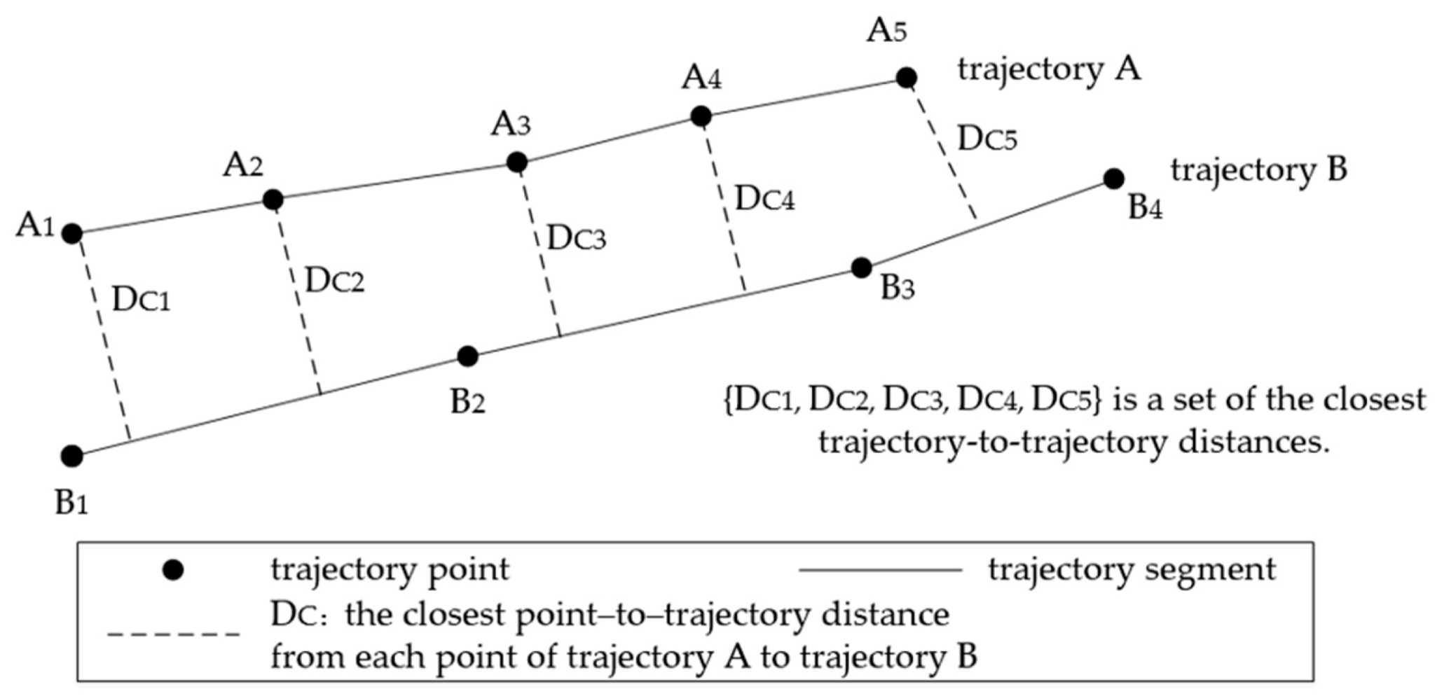
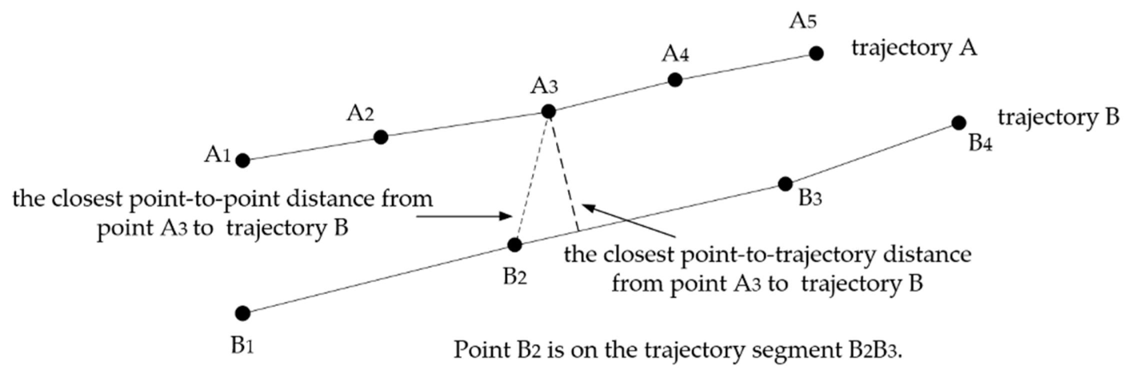
Definition (closest point-to-trajectory distance): Given a trajectory, where is a sample point, the closest point-to-trajectory distance (which may not be the orthographic projection distance) from to another trajectory S = is the shortest Euclidean distance from any point on S to
Definition (closest trajectory-to-trajectory distance): The closest trajectory-to-trajectory distance {} from trajectory to S = is the set of all the shortest Euclidean distances for each in.
2.1.3. Trajectory Similarity
Definition (trajectory similarity join): Given two trajectories, a similarity join aims to find all similar trajectory segment pairs in the two trajectories.
In this study, two parameters were mainly considered to determine the similarity of the trajectory pair: Distance similarity and angle similarity of the trajectory pair.
Definition (the similarity of two trajectory pairs): Given trajectories andsimilarity trajectories pair is defined by
where is distance similarity, is the closest distance between and, and is a fixed distance threshold. The value of is [0, 1]. The larger the value of, the larger the distance similarity. The value of is small, and the two trajectories are not similar. In Equation (2), is the angle similarity and is the maximum value of all angles. are the maximum values of the angles between the trajectory segment at which two trajectory points are located on and all the trajectory segments at which the closest points are located on . The smaller the value of, the closer the direction of the two trajectories. The larger the value of, the larger the parallelism.
Figure 1 depicts a schematic of the closest trajectory-to-trajectory distance.
2.2. Data Acquisition
In this study, we needed to acquire two types of trajectory data.
Type 1 includes the trajectory data of the road centerline. These data were obtained from an existing large-scale map with segment centerlines and without lane details. For example, professionally surveyed topographical maps of China at scales of 1:500 and 1:1000, as well as the National Geographic Information Survey of China, provide geographic information data that are expensive but high quality. The accuracy of the road network is relatively high and stable for a certain period of time. The accuracy of the road network in the map determines the final accuracy of the extracted lane-level road network. For example, if 0.5 m accuracy is assumed, the map would be at least 1:500. For this study, we used an existing road network data source with road centerline data accuracy greater than 0.5 m; the map was produced by professional surveying and mapping [29].
Type 2 includes the centerline of a specific lane in the direction of the road. These data were obtained from an autonomous vehicle. The autonomous vehicle drove along the centerline of any lane of the road with good accuracy by itself without previous centerline trajectory input and recorded the trajectory data. For calculation convenience, we took the centerline of the rightmost lane as an example. In this work, the positioning system of the autonomous vehicle combined GPS and high-precision inertial navigation system (INS). When collecting lane centerline trajectories, the vehicle traveled according to the lane centerline of the rightmost lane in the road traffic direction and completed the road network acquisition according to the Chinese map standard [36]. The coordinates of the acquisition trajectories and centerline trajectories of the road segments were geodetic coordinates, which are required for Gaussian projection when further processing data. Then, the plane coordinates were used in subsequent calculations.
3. Geometric-Based Approach for Inferring Lane-Level Road Networks
3.1. Overview
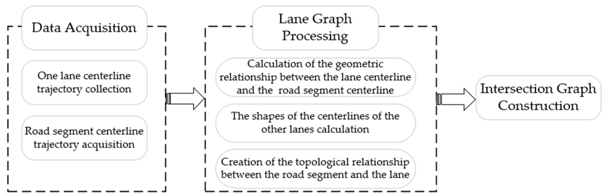
Once we finished data acquisition, we proceeded to lane graph processing. In this study, we used the centerline of the road to abstractly represent the lane-level road network. The geometric similarity between two roads is indicated by the similarity in geometric features that describe the two candidate roads, such as position, shape, and length [34]. In the same travel direction, the centerlines of multiple lanes are similar in shape and parallel to each other, with consistent separation between them. Generally, the widths of the lanes are the same in a given region. Therefore, the centerlines of the lanes and the centerline of the road are also similar in shape and parallel to each other. Based on prior studies, we mainly used the consistency of the direction and distance of the centerline of the road and the centerlines of the lanes to calculate the centerlines of other lanes in the same traffic direction. The entire lane-level road network generation process involved three steps, as shown in Figure 2: Data acquisition, lane graph processing, and intersection graph construction. In the following section, we describe these steps in detail.
3.2. Lane Graph Processing
The geometric representation of the road network may be divided into inferences of geometric shape and topographical connection. The lane graph processing proposed in this study has three steps: (1) Calculating the nearest estimated distance between the lane centerline trajectory and the road centerline trajectory, (2) calculating the centerline trajectory for other lanes using the simulation transformation model, and (3) generating the topological connection of the lane graph.
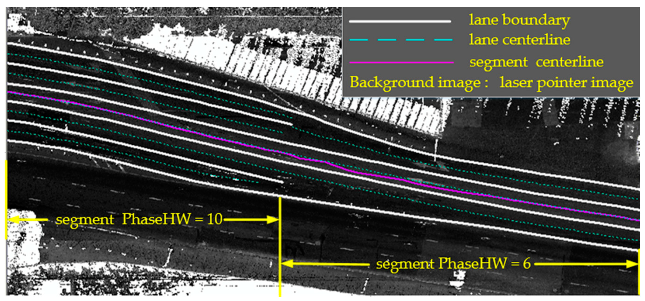
To calculate the closest trajectory to the trajectory distance between the outermost lane centerline trajectories and the road segment centerline trajectories in the same traffic direction, we first need to calculate the corresponding closest point on the road segment centerline trajectory segments. The road widths of the main roads of the city are relatively stable. Therefore, we can find the closest trajectory to a trajectory point aligned on the road segment centerline trajectories from the outermost lane centerline trajectories to the corresponding road segment centerline trajectories, which satisfies the spatial characteristic that the distance between the two lines of the segment should be consistent within a specific interval. Given the trajectory, where is a sample point, the calculated closest point to the trajectory distance from to another trajectory S = is, and is the closest point-to-trajectory distance. The lane width is defined as. We use PhaseHW to represent the number of half lane width metrics, as shown in Figure 3. According to the principle that road width is relatively stable within a certain range, PhaseHW satisfies Equation (3). The number of lanes in a road segment can be estimated using Equation (4):
To calculate the shape point of each lane center radiation transformation, we used a fixed-point formula. For the centerline lanes on the road segment, we used the segment centerline in the traffic direction as a boundary. The left-hand side of the road segment centerline is, and the right-hand side of the road segment centerline is . If the number of lanes is, conforms to Equation (5). Since is known, we can calculate and separately:
When is equal to 1, the acquisition trajectory by an autonomous vehicle is. If is more than 1, we need to calculate the remaining lane lines, except for the right-most lane, which is the acquisition trajectory. In Step 2, given the coordinates and, and using the parallel feature between the lane centerlines, the coordinates of the other lane trajectories in the vertical direction of the lane are sequentially obtained using the fixed-point formula. The fixed-point formula is expressed in Equations (6) and (7):
We sequentially and symmetrically transformed the trajectories of according to the sequence perpendicular to the direction of the road segment, which represents the trajectories of.
In the topological lane connection step, we used linear segmentation to organize the data and connect the generated road network topologically, as conducted in our previous research [29]. We first established the correspondence relationship between the lane and the road section, found the linear event point, and then established the topological connection of the lane graph.
3.3. Intersection Graph Construction
Virtual lanes are often used to express the traffic details of intersections in lane-level road maps [37]. Popular functions for describing lanes include the circular arc curve [38], clothoid curve [39], cubic Hermite curve [40], and B-spline curve [41]. We first determined the road sections that are included in the intersection and pass through a point adjacent to the road terminal. For a given traffic direction of a lane, we connected the centerlines of the lanes according to the rules for turning traffic. For topological expression, we used circular arc curves to describe the virtual lanes connected to the intersection [37].
4. TSJ Pruning-Based Algorithm for Inferring Lane Geometry
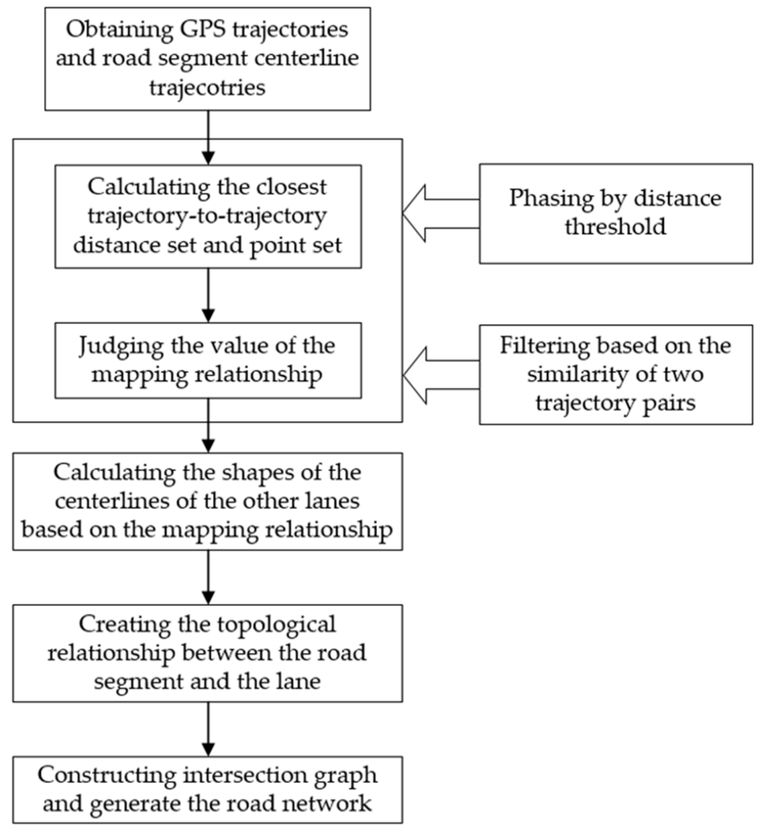
Given an acquisition trajectory and the road segment centerline trajectory of the centerline of the road, when calculating the trajectory of the remaining lane lines, the main operation is identifying the closest trajectory-to-trajectory point and the distance to the corresponding symmetrical point. The most critical factor is the need to quickly identify the closest trajectory-to-trajectory point between trajectories and. However, directly calculating the nearest trajectory-to-the trajectory point for every two trajectories is rather expensive. Therefore, we propose an algorithm that solves the problem of quickly identifying the nearest trajectory-to-trajectory point and the nearest distance. Our goal was to design a good filtering measure, find as many similar trajectory pairs as possible, and reduce the trajectory-to-trajectory distance-calculation candidate points. Figure 4 depicts the TSJ-pruning-based algorithm.
4.1. Algorithm Framework
The TSJ-PS method uses a filter-and-validation framework. We did not directly calculate each closest point to the trajectory distance. Instead of forming a rough candidate set-point pair through rough minimum distance, we obtained the PhaseHW corresponding to the candidate set-point pair for points with similar distances in the same interval. Further angle similarity judgment was conducted for point pairs with similar distances in the same interval, and similar points in the same interval were pruned. The point pairs in the coarse filtering candidate set were filtered to improve calculation efficiency. The true closest trajectory to the trajectory distance was then calculated, a new candidate set-point pair was formed, the new candidate set was subjected to PhaseHW division to check whether a new similarity point exists in the same interval, and the new candidate point pair was filtered again by trajectory similarity. Finally, the remaining result points that were not pruned were further calculated. The pseudo-code of the algorithm is provided in Algorithm 1.
| Algorithm 1 TSJ Pruning Based Framework |
| Input: lane centerline trajectory: T, road segment centerline trajectory: S, lane width: LaneWid, distance similarity: SimD, angle similarity: SimAng |
| Output: all lane centerline trajectory points |
| 1: compute AngT, AngS |
| 2: for each point in T do |
| 3: compute CandSetpd |
| 4: end for |
| 5: compute CandSubSetpd |
| 6: for point in CandSubSetpd and T do |
| 7: compute CandSubSetpp |
| 8: end for |
| 9: repeat filter in CandSubSetpp |
| 10: until CandSubSetpp |
| 11: compute LLane, RLane |
| 12: return all lane centerline trajectory points |
As shown in Algorithm 1, the TSJ-PS-based method first obtains the coarse filter candidate set by coarse filtering distance and then the coarse filter candidate set is filtered by trajectory similarity. This process is different from the original method presented in Section 2. Steps 2 and 5 filter pairs of trajectories with high similarity but little influence on the final accuracy, which prevents many redundant calculations in calculating the point-to-trajectory distance. In steps 9 and 10, the accurate candidate set-point pairs are updated, and the candidate set is subjected to secondary filtering. The candidate dataset is further filtered, which reduces the number of candidate datasets as well as the number of calculations in the affine transformation for the calculated lane centerline trajectories.
4.2. TSJ Pruning Strategy
4.2.1. Candidate Pair Fast Searching
To obtain all the lane centerlines of the road segment, we must first find the trajectory-to-trajectory distance between the rightmost lane centerline and the road segment centerline. This means that we must calculate each closest rightmost lane trajectory to the road centerline trajectory distance and the shortest distance points. We note that computing the minimal distance is expensive. According to the characteristics of Lemma 1, we first calculated the nearest point to the Euclidean distance between points in the rightmost lane centerline trajectory and in the road segment centerline trajectory instead of obtaining the nearest point-to-trajectory distance between them. This closest-point distance must pass the trajectory segment with the point closest to the trajectory distance.
Considering acquisition trajectory and road segment centerline trajectory, we must find a corresponding with the minimum Euclidean distance in for each, generating a set of nearest point distance candidate pairs (). should be sequenced, with no intersections in the spatiotemporal sequence.
Lemma 1.
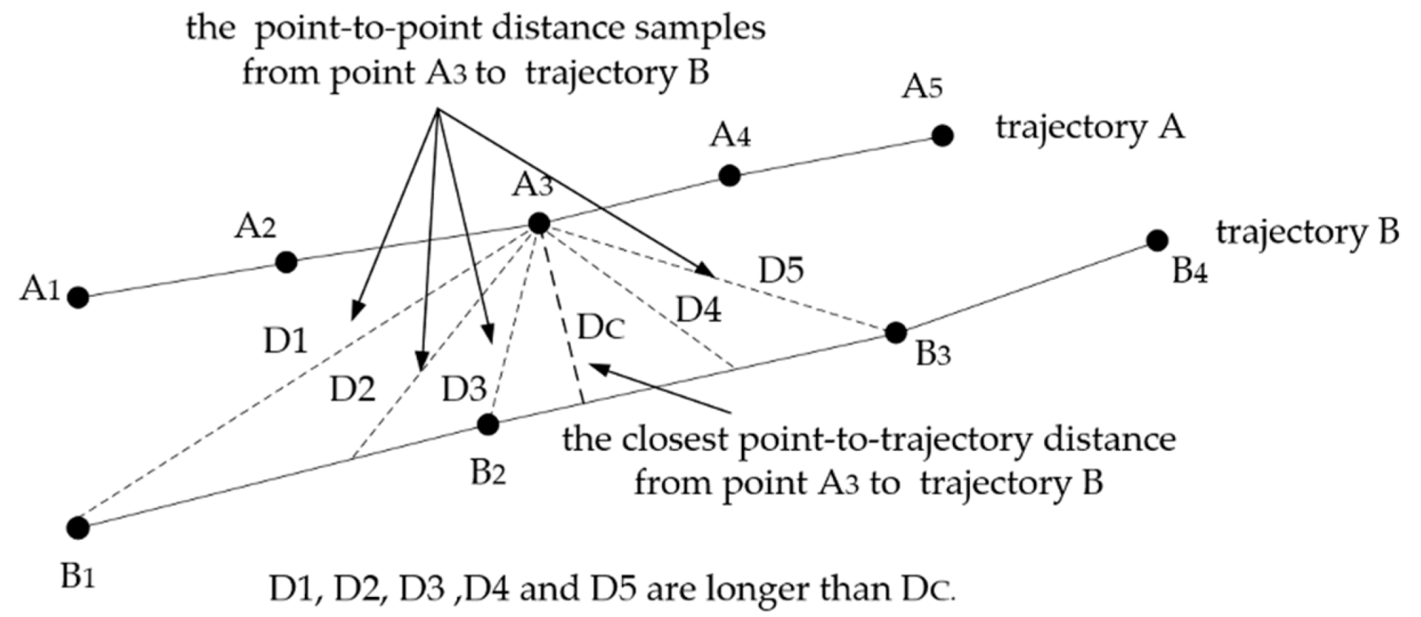
The trajectory segment with the closest point-to-trajectory distance passes through the nearest Euclidean distance point to the trajectory sample point [35]. As shown in Figure 5, point B2 is on the trajectory segment B2B3, which passes through the closest point-to-trajectory distance point from A3 to trajectory B.
4.2.2. TSJ Pruning Based on Different Distances
After the closest distance point pair is found, two adjacent trajectory segments exist. The vertical points on the two straight lines have to be calculated. Since this calculation is complicated, we needed to further streamline the calculations. Given the distance similarity threshold, if the trajectory pair satisfies Equation (8), the estimated pair distance is similar. According to Equation (3), we can obtain PhaseHW. In other words, consecutive segments with the same PhaseHW value are trajectory segments whose trajectories are similar in distance. Thus, for a given consecutive interval, the distances of the same PhaseHW in successive intervals are similar in distance.
If the trajectory pair satisfies Equations (8) and (9), the estimated pair is similar. The centerlines of the plurality of roads in the same traffic direction are similar in shape and have a segment-like relationship with the centerline of the road segment. When describing the shape of the road network, if the trajectory pairs are similar, we can use the first and last points of the trajectory pair to simplify the two trajectory pairs, as expressed in Equation (10):
According to Lemma 2 below, is the point-to-point distance and is the nearest point-to-segment distance on the segment. From Equation (4), we can obtain. If the same constitutes a continuous interval and the point pairs in the interval satisfy trajectory similarity, the interval composed of in the same interval is not necessarily continuous; however, the interval must satisfy the similarity of the region. Therefore, we can use the interval of the same value of for the similarity with which to assess the candidate interval of pruning. Given the nearest point distance candidate pairs of trajectory and, we calculate the set of by. In the same continuous interval, we perform similarity pruning and filter out track points smaller than the angle threshold. The candidate set after pruning is. The pseudo-code of the algorithm is provided in Algorithm 2.
Lemma 2.
| Algorithm 2 TSJ Pruning Algorithm |
| Input: lane centerline trajectory: T, road segment centerline trajectory: S, lane width: LaneWid, the set of the nearest point distance candidate pairs: CandSetpd, angle similarity: SimAng |
| Output: the candidate set after pruning: CandSubSetpd |
| 1: computer PhaseHwpd |
| 2: for each point in T do |
| 3: if there are more than 2 consecutive same PhaseHwpd then |
| 4: if trajectories are similar then |
| 5: delete points in the same PhaseHwpd interval |
| 6: update CandSetpd |
| 7: end if |
| 8: end if |
| 9: end for |
| 10: return CandSubSetpd |
4.2.3. Validation, Refinement, and Calculation
Given of the trajectories and , for each filtered point in T, we find the trajectory segment of trajectory according to the corresponding nearest point distance point and then calculate the nearest point-to-trajectory point. A new candidate pair is formed. The closest point is the required point for finding the centerline of the lane.
To reduce the amount of radiation conversion calculations and improve the storage efficiency of the road network, we further filter the candidate pair set without affecting accuracy. We calculate the new by using the same rule in Equations (9) and (10) to obtain the set of the closest point-to-trajectory distance points after pruning. The trajectory of the remaining lane center points is calculated using the formula provided in Section 2 by the filtered set. The pseudo-code of the algorithm is shown in Algorithm 3.
| Algorithm 3 Validation, Refinement, and Calculation |
| Input: angle similarity: SimAng, the candidate set after pruning: CandSubSetpd, distance similarity: SimD, lane centerline trajectory: T, road segment centerline trajectory: S |
| Output: all lane centerline trajectory points |
| 1: computer CandSetpp |
| 2: computer PhaseHwpp |
| 3: for each point in CandSetpp do |
| 4: if there are more than 2 consecutive same PhaseHwpp then |
| 5: if trajectories are similar then |
| 6: delete points in the same PhaseHwpp interval |
| 7: update CandSetpp |
| 8: end if |
| 9: end if |
| 10: end for |
| 11: CandSubSetpp ← CandSetpp |
| 12: compute LLane, RLane |
| 13: return all lane centerline trajectory points |
4.3. Time Complexity Analysis of the Algorithm
The time complexity of the TSJ-pruning-based algorithm is the sum of the time complexities in steps 1–10 of Algorithm 1 in Section 4.1. Among them, the time complexity of the fast search candidate pairs in step 2 is from Section 4.2.1, and the TSJ pruning is based on different distances in step 5 from Section 4.2.2; that of the validation, refinement, and calculation time complexity in steps 6–10 is from Section 4.2.3. Therefore, the total time complexity is, where represents the number of sample points of trajectory, is the number of sample points of trajectory, the number of, and is the number of.
5. Experiments
5.1. Data and Experimental Setting
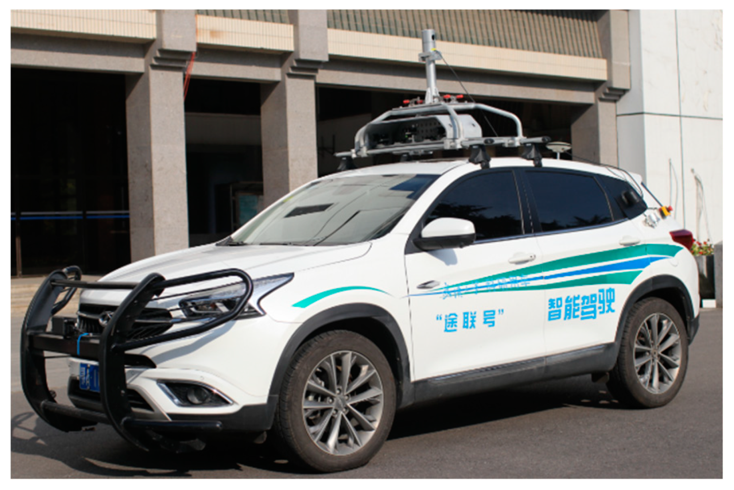
The experimental data were collected by an autonomous vehicle equipped with positioning equipment to collect lane-level road network data. The configuration of the experimental car, acquisition process, and map-digitization process were consistent with those of a previous study [29]. Figure 7 depicts the experimental car. The positioning system of the vehicle was a NovAtel SPAN-FSAS inertial integrated navigation system (NovAtel Inc., Calgary, Canada). Its positioning accuracy can reach 2 cm. The system provides a root mean square (RMS) of roll of 0.015°, an RMS of the pitch angle of 0.015°, an RMS of the heading of 0.040°, and was designed with 200 Hz frequency for raw data acquisition. In this study, the data update frequency of the NovAtel SPAN-FSAS was 100 Hz.
The programming language chosen for the experiment was Python 3, and the computer used for the experiment was a 3.60 GHz Intel Core CPU (Central Processing Unit) i7-7700 (Intel, California, USA) with 8.00 GB of RAM (Random Access Memory) running Windows 7 (Microsoft Corporation, Redmond, WA, USA).
5.2. Generation of Lane-Level Road Network
5.2.1. Experimental Data Acquisition
For the experiment, we selected an actual road section in Shanghai as the testing area. The survey area covered 11.6 km and contained 36 road sections. Prior to the start of the experiment, we used the experimental vehicle and mobile measurement technology to create a high-precision lane-level map [27]. Since the purpose of this study was to demonstrate the proposed algorithm, we were not concerned with how to implement high-precision map production algorithms using mobile measurement techniques. In the survey area, the road network in the easterly direction had a maximum error of 0.134 m and a minimum error of 0.003 m. In the northerly direction, the road network had a maximum error of 0.121 m and a minimum error of 0.003 m. The mean square error (MSE) in the plane was ±0.043 m. We used the centerline data of the lanes in the high-precision map as the true values to which we compared the experimental data.
To conduct the experiments, we needed to obtain two different types of data: The centerline trajectory data of the road segment and the lane centerline trajectory data of the lanes. In addition, the accuracy of the collected trajectories in the experiment played a decisive role in the accuracy of the generated lane centerline trajectories. Therefore, we needed to evaluate the accuracy of the trajectory.
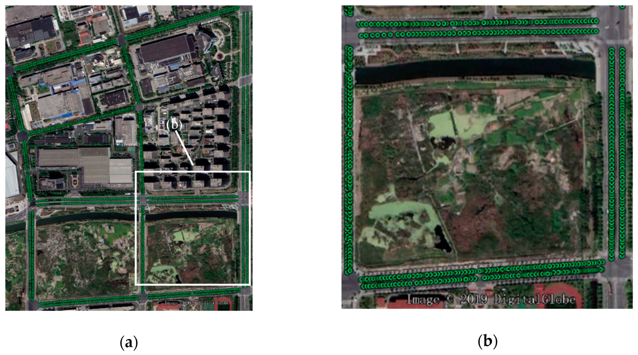
The first type of experimental data to be acquired and assessed for accuracy was the centerline trajectory data of the road segment. We used the road network of the high-precision map as the first type of experimental data. The experimental test area contained 2665 road segment centerline trajectories. Since the available experimental methods could not generate data with higher precision than the map, it was not possible to evaluate the accuracy of the centerline trajectory of the road sections. We used the accuracy of the map as a substitute for the accuracy of the road network. The accuracy of the centerline of the road network has a MSE of ±0.043 m. Figure 8 shows all road segment centerline trajectories and the enlarged map.
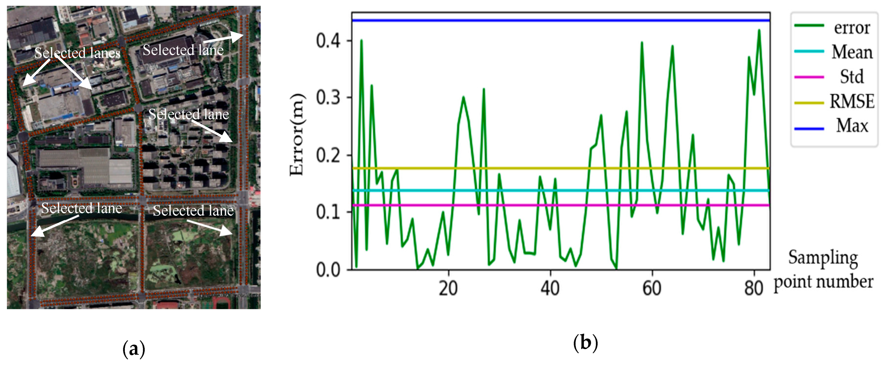
The second type of experimental data to be acquired was the lane centerline data. We used the unmanned vehicle to collect the centerline data of the rightmost lane. A total of 939 GPS points were collected, as shown in Figure 9a. The data were acquired according to the Chinese map standard. The accuracy of the input data in the algorithm can affect the final accuracy of the road network. Therefore, we calculated accuracy by comparing the centerline data of the lanes in the high-precision map with the trajectory data of the unmanned vehicle. To evaluate the accuracy of the collection point instead of the rightmost road centerline, we calculated the mean error (Mean), standard deviation error (Std), root mean square error (RMSE), and maximum error (Max) between the collected trajectories and the true rightmost lane centerline. We randomly selected six trajectory pairs for the experiment. The comparison results are shown in Figure 9b.
5.2.2. Visualization of Road Network Graphics
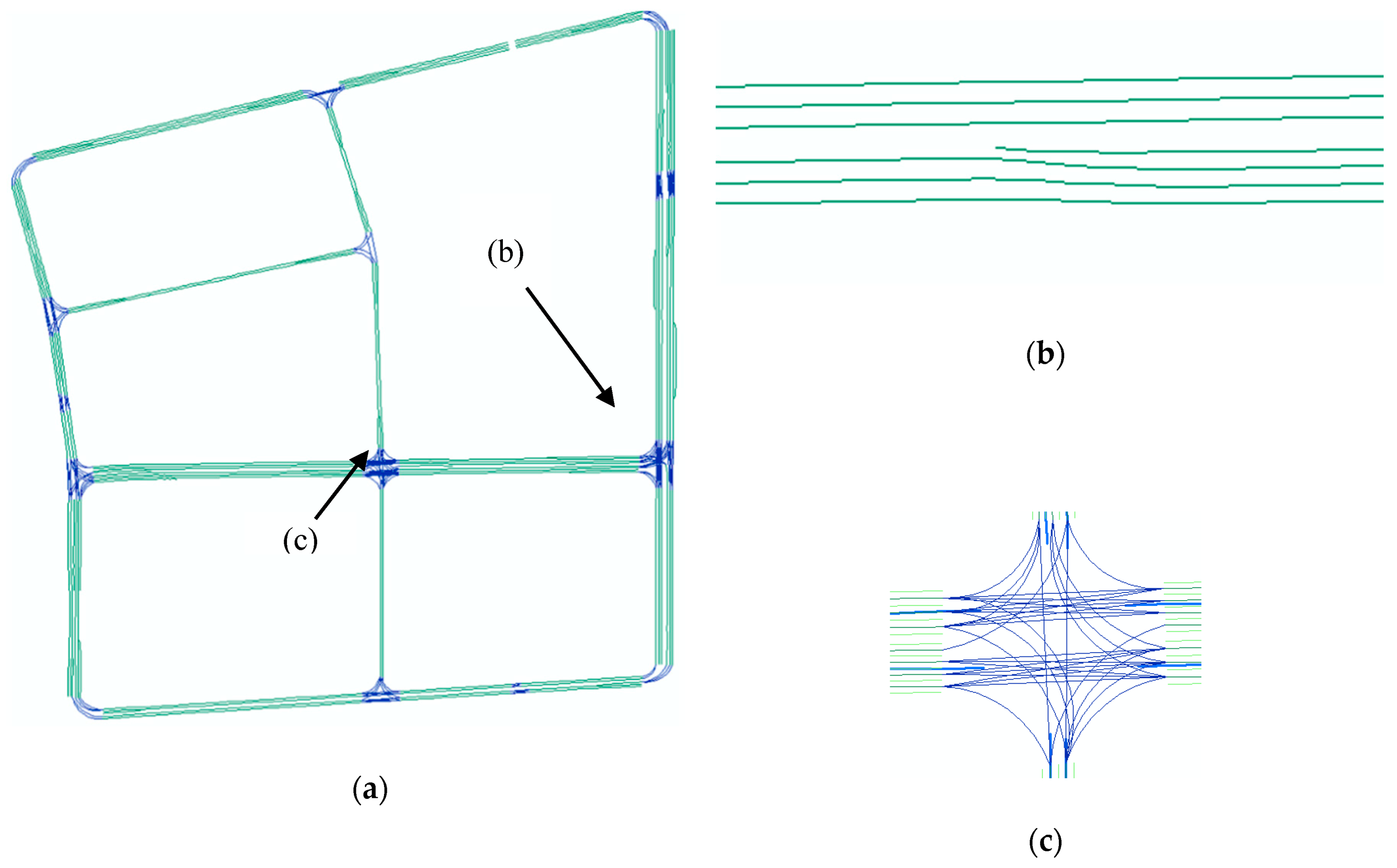
We used the TSJ-pruning-based algorithm method proposed in this paper to calculate the data for all sections in the area and to generate the road network. The widths of the given lanes were 2 and 4 m, the similarity of distance was 0.85, and the similarity of angle was 0.97. Figure 10a shows the lane-level road network generation results. Figure 10b provides a detailed view of one of the road segments after enlargement, and Figure 10c depicts the enlarged intersection. To maintain the integrity of the road network, we manually connected the traffic direction line at the intersection.
5.3. Performance of the TSJ-PS-Based Algorithm
5.3.1. Adopted Comparison Algorithm
To test our TSJ-PS-based extraction algorithm, we compared our method with two other methods.
The first comparative experimental algorithm did not use pruning, calculated the closest trajectory and trajectory distance points, and then generated the lane centerline trajectory.
The second comparative experimental algorithm used a grid-based method [9]. This method uses an orthographic projection but is based on a grid structure. Specifically, grid signatures were generated for the GPS collection trajectory and lane centerline trajectory, and the nearest road segment centerline trajectory grid points within the distance threshold were found and formed the candidate set. Similarity filtering on the candidate set was then performed and the closest point-to-trajectory distance point based on the point of the candidate set after pruning was calculated. Finally, we calculated the lane centerline coordinates using the method presented in Section 2. The pseudo-code of the algorithm is provided in Algorithm 4.
| Algorithm 4 grid-based Algorithm |
| Input: lane centerline trajectory: T, road segment centerline trajectory: S, lane width: LaneWid |
| Output: all lane centerline trajectory points |
| 1: computer GridStep |
| 2: computer GridT, GridS |
| 3: computer AngT, AngS |
| 4: computer BoundaryCoorS |
| 5: for each point in GridT do |
| 6: compute NearestPoint |
| 7: compute filterindex |
| 8: end for |
| 9: computer vertical point in filterindex |
| 10: computer all lane centerline trajectory points |
| 11: return all lane centerline trajectory points |
5.3.2. Accuracy Evaluation of Road Network Graphics
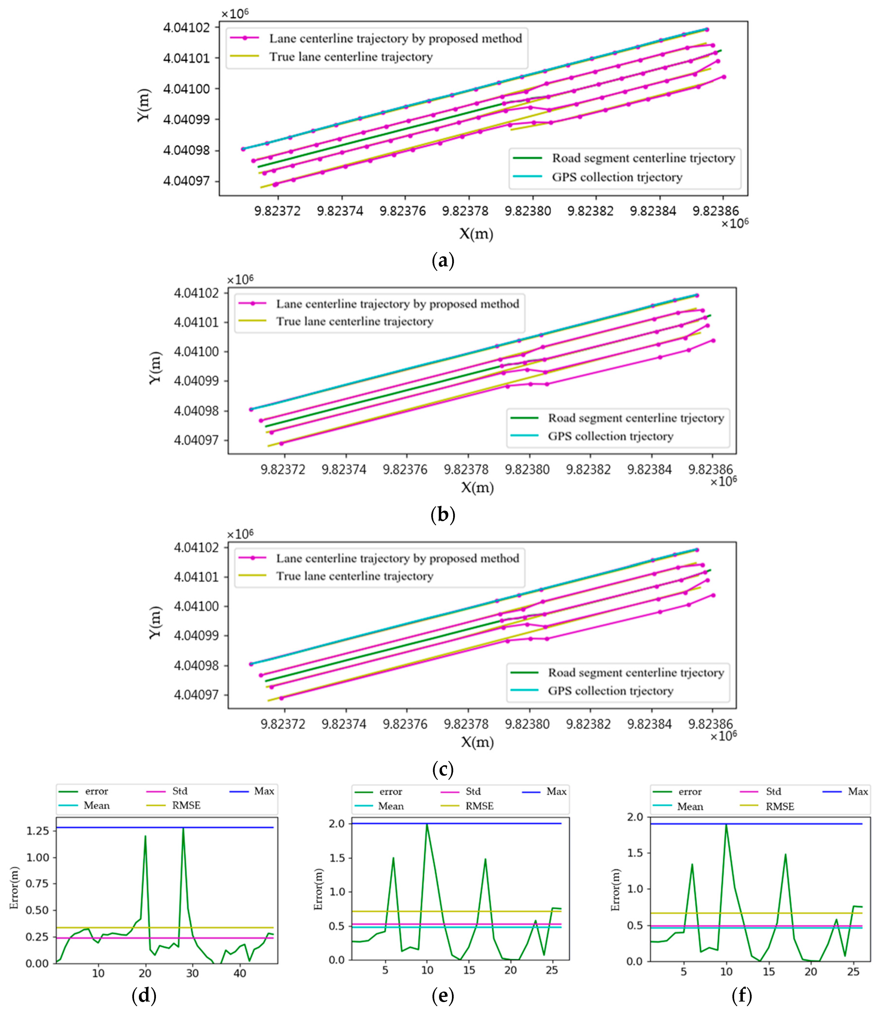
To further evaluate the accuracy of the lanes in a single section of road, the error-detailed views of one segment analysis (Figure 11a–c) created by the three methods were generated separately, and error analysis tables were generated (Figure 11d–f). In the experiment, we set the width of the lane to 4 m.
Using the three methods, we conducted experiments on the entire area and evaluated the accuracy of the road networks that were generated. To achieve the best experimental results, using the method proposed in this paper, we set the widths of the lanes to 2 and 4 m, the distance similarity to 0.85, and the angle similarity to 0.97. In the grid-based method, the widths of the lane were 2.2 and 4 m, the distance similarity was 0.86, and the angle similarity was 0.97. We then calculated the Mean, Std, RMSE, and Max errors between the lane centerline coordinates generated by the three experiments and the true value coordinates. The accuracy evaluation results for the entire experimental area are shown in Table 1.
5.3.3. Algorithm Efficiency
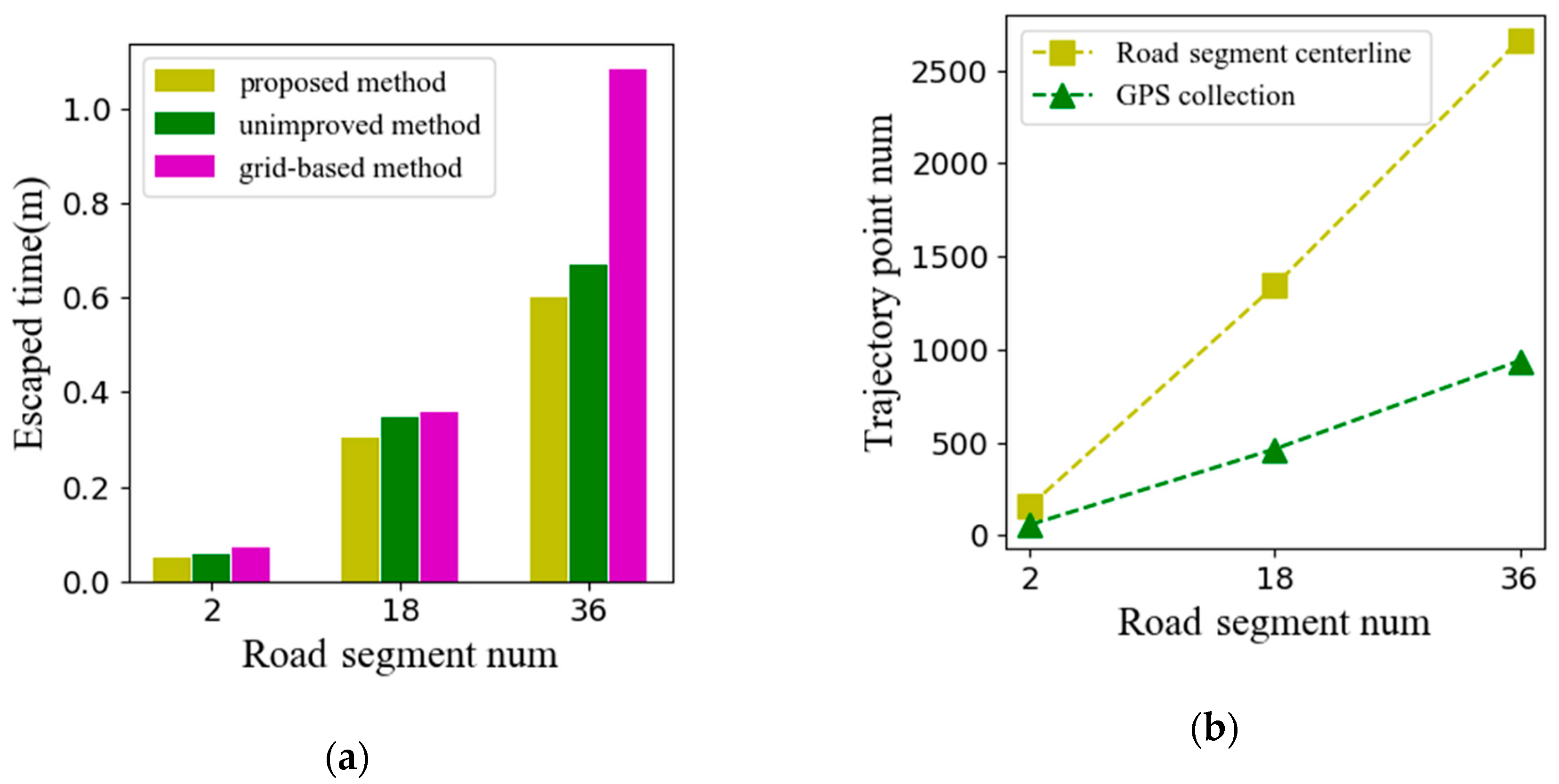
To observe the computational efficiency of the algorithm for different data volumes and the stability of the algorithm, we selected three different road numbers as our experimental data. The road segment numbers of the three experimental datasets were 2, 18, and 36, which were tested using the unimproved, grid-based, and proposed methods. To obtain the best experimental results, in the experiment using the method proposed in this paper, the width of the lane was 2 m, the distance similarity was 0.85, and the angle similarity was 0.97. For the grid-based method, the width of the lane was 2.2 m, the distance similarity was 0.86, and the angle similarity was 0.97. Figure 12a shows the elapsed time for the three algorithms under different data quantities, and Figure 12b shows the number of collection trajectories and the number of road centerline trajectories with different road segment numbers.
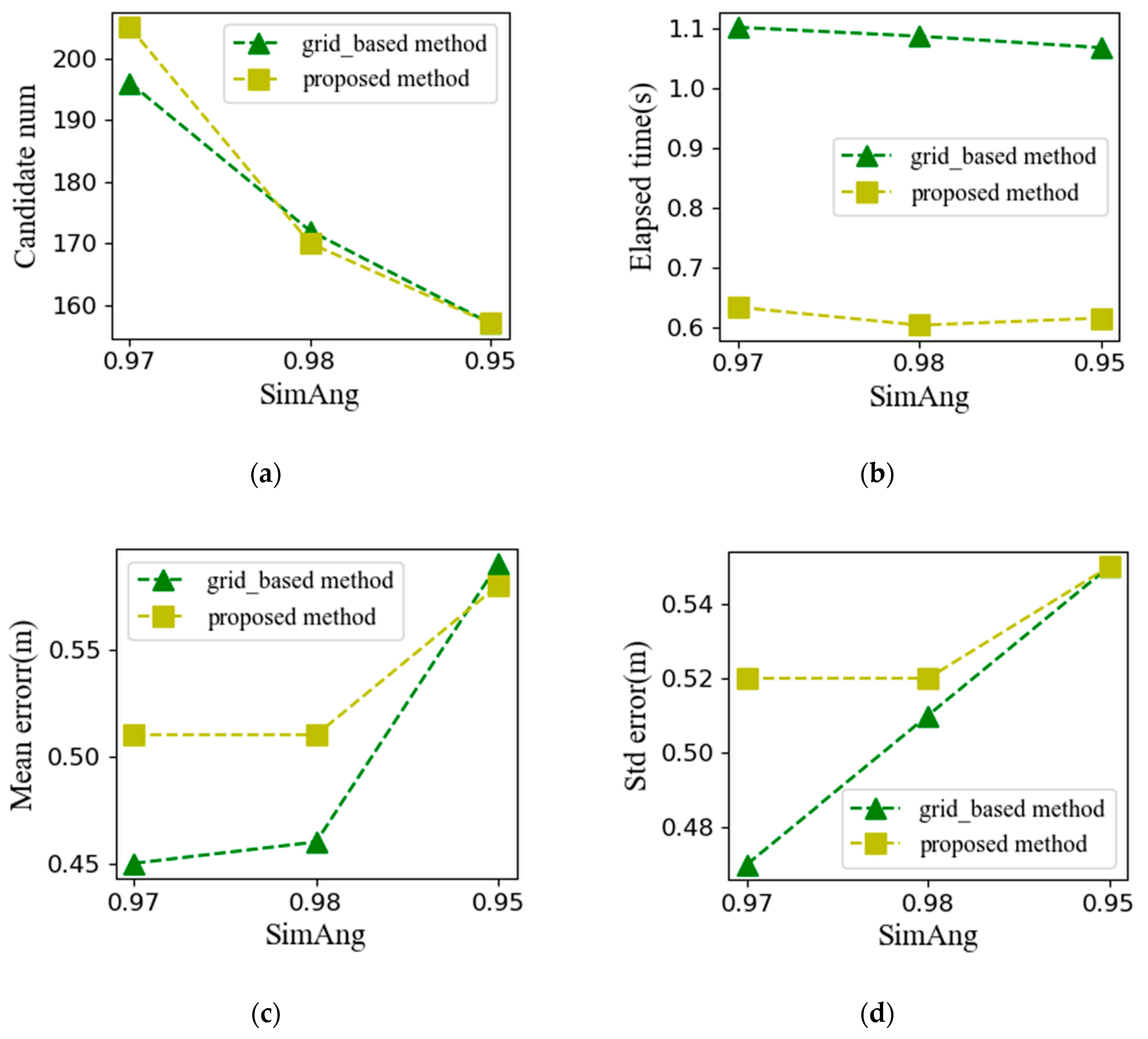
5.3.4. Effect of Similarity of Angles (SimAng)
To test the effect of the similarity of angles, we chose the method proposed in this paper and the grid-based method, and used three angle similarities to test the entire experimental dataset for each method. The size of the candidate set, the elapsed time, and the correct rate of the experimental results were recorded. In these experiments, for the experiment using the proposed method, the width of the lane was 2 m and the distance similarity was 0.85. In the experiment using the grid-based method, the width of the lane was 2.2 m and the distance similarity was 0.85. Figure 13 depicts all the experimental results.
6. Discussion
The experimental results presented in Section 5.2 verify the effectiveness of the algorithm and show that the proposed method generated a lane-level road network based on collecting point trajectories and road network trajectories in an existing map.
The results in Section 5.2.1 show that the maximum accuracy of the acquisition point instead of the rightmost lane was less than 0.4 m, indicating that the road acquisition process accurately calculated the lane trajectory. The overall accuracies of the three algorithms were relatively close and consistent with the accuracy requirements of lane-level road networks.
However, the accuracy of the unimproved algorithm was higher because the higher the density of the sample points, the higher the accuracy of the road network. In addition, the unimproved algorithm was more accurate when the lane shape change was relatively small because the fitting accuracy of a straight line is higher than that of a curve. When the number of lanes increased but the lane width was almost constant, the three algorithms could extract the correct number of lanes due to the effectiveness of the algorithm and because the data acquisition process provided good raw acquisition trajectories.
The results in Section 5.3.3 show that the proposed method is more efficient than the unimproved and grid-based methods, thus highlighting the effectiveness of the trajectory similarity pruning strategy. The grid-based method also performs pruning, but it consumes more computing resources, which decreases the efficiency of the entire algorithm. With the expansion of the data scale, the three methods generally showed a linear upward trend. The efficiencies of the three methods were relatively stable when using small-scale data. We can speculate that for road data, the larger the data size, the more efficient the pruning efficiency over time. We can infer that the algorithm is more efficient at changing the shape of the lane when the lane shape change is relatively small because the algorithm has a better effect on pruning when the road condition changes are relatively small.
The results in Section 5.3.4 indicate that the larger the SimAng value, the greater the similarity between the line segments and the less obvious the pruning effect. The smaller the SimAng value, the more dissimilar candidate points are selected and, thus, the higher the correction rate. The proposed and grid-based algorithms showed little differences in pruning and could basically reduce the number of lane trajectories.
7. Conclusions
This study proposed a method for using acquisition trajectories and road centerline shape points to generate a lane-level road network. The main contribution of this study is that we used the existing acquisition platform of an autonomous vehicle as one data source and professionally surveyed road centerline data of an existing road-level network as another source. This approach effectively uses unmanned vehicle data and provides a new method for map manufacturers to produce lane-level road networks only using position data. We also proposed a TSJ-PS algorithm that can quickly and effectively generate the lane centerline trajectories of the lane-level road network, providing a solution for generating and updating map data for real-time online updates. This study demonstrated the effectiveness of the proposed method using experimental data for a real road.
Currently, autonomous vehicles are developing rapidly, and the combination of car networking technology and autonomous driving technology is expected to realize real-time intercommunication of information in entire regions. In the environment of the Internet of Autonomous Vehicles, autonomous vehicles with communication capabilities are important sources for road network data. This study has helped to solve the problem of lane-level road network generation using a single autonomous car as an intelligent crowd-sensing agent. This study provides a foundation for future research and development of high-precision road networks based on crowd sensing in the Internet of Vehicles.
Author Contributions
This research was jointly conducted by all of the authors. Bijun Li and Ling Zheng primarily designed and conducted the experiments. Ling Zheng performed the experiments and wrote the paper. Huashan Song helped with the experimental design. Hongjuan Zhang collected the experimental data statistics.
Funding
This research was funded by the National Natural Science Foundation of China (grant nos. 41671441, 41531177, and U1764262).
Conflicts of Interest
The authors declare that they have no conflict of interest.
References
- Brubaker, M.A.; Geiger, A.; Urtasun, R. Map-Based Probabilistic Visual Self-Localization. IEEE Trans. Pattern Anal. Mach. Intell. 2016, 38, 652–665. [Google Scholar] [CrossRef] [PubMed]
- Gruyer, D.; Belaroussi, R.; Revilloud, M. Accurate lateral positioning from map data and road marking detection. Expert Syst. Appl. 2016, 43, 1–8. [Google Scholar] [CrossRef]
- Dominguez, S.; Khomutenko, B.; Garcia, G.; Martinet, P. An Optimization Technique for Positioning Multiple Maps for Self-Driving Car’s Autonomous Navigation. In Proceedings of the 2015 IEEE 18th International Conference on Intelligent Transportation Systems, Las Palmas, Spain, 15–18 September 2015; pp. 2694–2699. [Google Scholar]
- Chen, S.; Shang, J.; Zhang, S.; Zheng, N. Cognitive Map-Based Model: Toward A Developmental Framework for Self-Driving Cars. In Proceedings of the 2017 IEEE 20th International Conference on Intelligent Transportation Systems (ITSC), Yokohama, Japan, 16–19 October 2017; pp. 1–8. [Google Scholar]
- Yoneda, K.; Yanase, R.; Aldibaja, M.; Suganuma, N.; Sato, K. Mono-Camera Based Vehicle Localization Using Lidar Intensity Map for Automated Driving. Artif. Life Robot. 2019, 24, 147–154. [Google Scholar] [CrossRef]
- Häne, C.; Lee, G.H.; Fraundorfer, F.; Furgale, P.; Sattler, T.; Pollefeys, M.; Heng, L. 3D visual perception for self-driving cars using a multi-camera system: Calibration, mapping, localization, and obstacle detection. Image Vis. Comput. 2017, 68, 14–27. [Google Scholar] [CrossRef] [Green Version]
- Editorial Department on China Journal of Highway and Transport. Review on China’s Automotive Engineering Research Progress:2017. Chin. J. Highw. Transp. 2017, 30, 1–197. [Google Scholar]
- Liu, C.; Jiang, K.; Yang, D.; Xiao, Z. Design of a multi-layer lane-level map for vehicle route planning. In Proceedings of the MATEC Web of Conferences, Hong Kong, China, 1–3 July 2017; p. 03001. [Google Scholar]
- Wang, M.; Guo, B.; Li, D.; Gong, J. Multiple Sensors and Road Network Used for Mobile Navigating. Geomat. Inf. Sci. Wuhan Univ. 2001, 26, 205–208. [Google Scholar]
- Poggenhans, F.; Pauls, J.-H.; Janosovits, J.; Orf, S.; Naumann, M.; Kuhnt, F.; Mayr, M. Lanelet2: A high-definition map framework for the future of automated driving. In Proceedings of the 2018 21st International Conference on Intelligent Transportation Systems (ITSC), Maui, HI, USA, 4–7 November 2018; pp. 1672–1679. [Google Scholar]
- Jiang, K.; Yang, D.; Liu, C.; Zhang, T.; Xiao, Z. A Flexible Multi-Layer Map Model Designed for Lane-Level Route Planning in Autonomous Vehicles. Engineering 2019, 5, 305–318. [Google Scholar] [CrossRef]
- Ma, L.; Li, Y.; Li, J.; Wang, C.; Wang, R.; Chapman, M.A. Mobile Laser Scanned Point-Clouds for Road Object Detection and Extraction: A Review. Remote Sens. 2018, 10, 1531. [Google Scholar] [CrossRef]
- Wu, T.; Xiang, L.; Gong, J. Updating Road Networks by Local Renewal from GPS Trajectories. ISPRS Int. J. Geo-Inf. 2016, 5, 163. [Google Scholar] [CrossRef]
- Li, L.; Li, D.; Xing, X.; Yang, F.; Rong, W.; Zhu, H. Extraction of Road Intersections from GPS Traces Based on the Dominant Orientations of Roads. ISPRS Int. J. Geo-Inf. 2017, 6, 403. [Google Scholar] [CrossRef]
- Yang, X.; Tang, L.; Niu, L.; Zhang, X.; Li, Q. Generating lane-based intersection maps from crowdsourcing big trace data. Transp. Res. Part C Emerg. Technol. 2018, 89, 168–187. [Google Scholar] [CrossRef]
- Uduwaragoda, E.; Perera, A.; Dias, S. Generating lane level road data from vehicle trajectories using kernel density estimation. In Proceedings of the 16th International IEEE Conference on Intelligent Transportation Systems (ITSC 2013), The Hague, The Netherlands, 6–9 October 2013; pp. 384–391. [Google Scholar]
- Chen, Z.; Ellis, T. Automatic lane detection from vehicle motion trajectories. In Proceedings of the 2013 10th IEEE International Conference on Advanced Video and Signal Based Surveillance, Krakow, Poland, 27–30 August 2013; pp. 466–471. [Google Scholar]
- Chen, Z.; Yan, Y.; Ellis, T. Lane detection by trajectory clustering in urban environments. In Proceedings of the 17th International IEEE Conference on Intelligent Transportation Systems (ITSC), Qingdao, China, 8–11 October 2014; pp. 3076–3081. [Google Scholar]
- Qiu, J.; Wang, R. Road Map Inference: A Segmentation and Grouping Framework. ISPRS Int. J. Geo-Inf. 2016, 5, 130. [Google Scholar] [CrossRef]
- Yang, X.; Tang, L.; Stewart, K.; Dong, Z.; Zhang, X.; Li, Q. Automatic change detection in lane-level road networks using GPS trajectories. Int. J. Geogr. Inf. Sci. 2018, 32, 601–621. [Google Scholar] [CrossRef]
- Jo, K.; Sunwoo, M. Generation of a Precise Roadway Map for Autonomous Cars. IEEE Trans. Intell. Transp. Syst. 2013, 15, 925–937. [Google Scholar] [CrossRef]
- Betaille, D.; Toledo-Moreo, R. Creating Enhanced Maps for Lane-Level Vehicle Navigation. IEEE Trans. Intell. Transp. Syst. 2010, 11, 786–798. [Google Scholar] [CrossRef]
- Yang, L.; Cheng, X.; Ghogho, M.; Ayanoglu, E.; Huang, T.; Zheng, N. Guest Editorial Special Issue on IoT on the Move: Enabling Technologies and Driving Applications for Internet of Intelligent Vehicles (IoIV). IEEE Internet Things J. 2019, 6, 1–5. [Google Scholar] [CrossRef]
- Ge, X. Ultra-Reliable Low-Latency Communications in Autonomous Vehicular Networks. IEEE Trans. Veh. Technol. 2019, 68, 5005–5016. [Google Scholar] [CrossRef] [Green Version]
- Liu, J.; Wang, H.; Guo, C.; Zhang, H.; Zuo, W.; Yang, C. Progress and Consideration of High Precision Road Navigation Map. Eng. Sci. 2018, 20, 99–105. [Google Scholar] [CrossRef]
- Gwon, G.-P.; Hur, W.-S.; Kim, S.-W.; Seo, S.-W. Generation of a Precise and Efficient Lane-Level Road Map for Intelligent Vehicle Systems. IEEE Trans. Veh. Technol. 2017, 66, 4517–4533. [Google Scholar] [CrossRef]
- Guo, C.; Kidono, K.; Meguro, J.; Kojima, Y.; Ogawa, M.; Naito, T. A Low-Cost Solution for Automatic Lane-Level Map Generation Using Conventional In-Car Sensors. IEEE Trans. Intell. Transp. Syst. 2016, 17, 2355–2366. [Google Scholar] [CrossRef]
- Zhang, T.; Arrigoni, S.; Garozzo, M.; Yang, D.-G.; Cheli, F. A lane-level road network model with global continuity. Transp. Res. Part C: Emerg. Technol. 2016, 71, 32–50. [Google Scholar] [CrossRef]
- Zheng, L.; Li, B.; Zhang, H.; Shan, Y.; Zhou, J. A High-Definition Road-Network Model for Self-Driving Vehicles. ISPRS Int. J. Geo-Inf. 2018, 7, 417. [Google Scholar] [CrossRef]
- Bernhardsen, T. Geographic Information Systems: An Introduction; John Wiley & Sons: New York, NY, USA, 2002. [Google Scholar]
- Chehreghan, A.; Abbaspour, R.A. An Assessment of The Efficiency of Spatial Distances in Linear Object Matching on Multi-Scale, Multi-Source Maps. Int. J. Image Data Fusion 2017, 9, 95–114. [Google Scholar] [CrossRef]
- Mao, Y.; Zhong, H.; Xiao, X.; Li, X. A Segment-Based Trajectory Similarity Measure in the Urban Transportation Systems. Sensors 2017, 17, 524. [Google Scholar] [CrossRef] [PubMed]
- Zhang, J.; Wang, Y.; Zhao, W. An Improved Probabilistic Relaxation Method for Matching Multi-Scale Road Networks. Int. J. Digit. Earth 2018, 11, 635–655. [Google Scholar] [CrossRef]
- Xing, R.; Wu, F.; Zhang, H.; Gong, X. Dual-carriageway Road Extraction Based on Facing Project Distance. Geomat. Inf. Sci. Wuhan Univ. 2018, 43, 152–158. [Google Scholar] [CrossRef]
- Ta, N.; Li, G.; Xie, Y.; Li, C.; Hao, S.; Feng, J. Signature-Based Trajectory Similarity Join. IEEE Trans. Knowl. Data Eng. 2017, 29, 870–883. [Google Scholar] [CrossRef]
- Cao, X.; Xu, J.; Chen, D.; Lü, Y.; Xu, J.; Li, L.; Li, B.; Zheng, L.; Li, M.; Liu, B.; et al. Framework Data Exchange Format for Navigation Electronic Map; Standards Press of China: Beijing, China, 2017. [Google Scholar]
- Zhang, T.; Yang, D.; Li, T.; Li, K.; Lian, X. An improved virtual intersection model for vehicle navigation at intersections. Transp. Res. Pt. C-Emerg. Technol. 2011, 19, 413–423. [Google Scholar] [CrossRef]
- Schindler, A.; Maier, G.; Pangerl, S. Exploiting arc splines for digital maps. In Proceedings of the 2011 14th International IEEE Conference on Intelligent Transportation Systems (ITSC), Washington, DC, USA, 5–7 October 2011; pp. 1–6. [Google Scholar]
- Brisan, C.; Vasiu, R.-V.; Munteanu, L. A modular road auto-generating algorithm for developing the road models for driving simulators. Transp. Res. Part C: Emerg. Technol. 2013, 26, 269–284. [Google Scholar] [CrossRef]
- Chen, A.; Ramanandan, A.; Farrell, J.A. High-precision lane-level road map building for vehicle navigation. In Proceedings of the IEEE/ION Position, Location and Navigation Symposium, Indian Wells, CA, USA, 4–6 May 2010; pp. 1035–1042. [Google Scholar]
- Jo, K.; Lee, M.; Kim, C.; Sunwoo, M. Construction process of a three-dimensional roadway geometry map for autonomous driving. Proc. Inst. Mech. Eng. Part D J. Automob. Eng. 2017, 231, 1414–1434. [Google Scholar] [CrossRef]
Figure 1.
Schematic of the closest trajectory-to-trajectory distance.

Figure 2.
Framework of the geometric-based approach.

Figure 3.
Example of the PhaseHW (the number of half lane width metrics) of a real world segment.

Figure 4.
TSJ-pruning-based algorithm. Note: Global positioning system (GPS) and trajectory-similarity-join (TSJ).
Figure 4.
TSJ-pruning-based algorithm. Note: Global positioning system (GPS) and trajectory-similarity-join (TSJ).

Figure 5.
Illustration of Lemma 1.

Figure 6.
Illustration of Lemma 2.

Figure 7.
Autonomous vehicle equipped with positioning equipment for experiment.

Figure 8.
Experimental area and raw data: (a) Road segment centerline points; (b) enlarged road segment centerline raw trajectories.
Figure 8.
Experimental area and raw data: (a) Road segment centerline points; (b) enlarged road segment centerline raw trajectories.

Figure 9.
Experimental area and raw data: (a) GPS collection raw points; (b) accuracy assessment of original GPS trajectories. Note: Mean error (Mean), standard deviation error (Std), root mean square error (RMSE), and maximum error (Max).
Figure 9.
Experimental area and raw data: (a) GPS collection raw points; (b) accuracy assessment of original GPS trajectories. Note: Mean error (Mean), standard deviation error (Std), root mean square error (RMSE), and maximum error (Max).

Figure 10.
Generation of lane-level road network results: (a) Lane-level road network generation results; (b) enlarged road network segments; and (c) enlarged map of intersection.
Figure 10.
Generation of lane-level road network results: (a) Lane-level road network generation results; (b) enlarged road network segments; and (c) enlarged map of intersection.

Figure 11.
Errors between the true road segment lane trajectories and lane trajectories generated by (a,d) unimproved; (b,e) grid-based; and (c,f) the proposed algorithms.
Figure 11.
Errors between the true road segment lane trajectories and lane trajectories generated by (a,d) unimproved; (b,e) grid-based; and (c,f) the proposed algorithms.

Figure 12.
Algorithm efficiency results: (a) Elapsed time under different data quantities obtained by unimproved, grid-based, and proposed algorithms; (b) number of collection trajectories and number of road centerline trajectories with different road segment numbers.
Figure 12.
Algorithm efficiency results: (a) Elapsed time under different data quantities obtained by unimproved, grid-based, and proposed algorithms; (b) number of collection trajectories and number of road centerline trajectories with different road segment numbers.

Figure 13.
Similarity of angle (SimAng) effect results: (a) Candidate set size; (b) elapsed time; and (c,d) accuracy of the grid-based algorithm and the proposed algorithm with different SimAng values.
Figure 13.
Similarity of angle (SimAng) effect results: (a) Candidate set size; (b) elapsed time; and (c,d) accuracy of the grid-based algorithm and the proposed algorithm with different SimAng values.


Table 1.
Errors between all true road segment lane trajectories in the experimental area and the lane trajectories generated by the unimproved, grid-based, and proposed algorithms.
Table 1.
Errors between all true road segment lane trajectories in the experimental area and the lane trajectories generated by the unimproved, grid-based, and proposed algorithms.
| Method | Mean (m) | Std (m) | RMSE (m) | Max (m) |
|---|---|---|---|---|
| Unimproved | 0.37 | 0.43 | 0.57 | 1.89 |
| Grid-based | 0.46 | 0.51 | 0.63 | 1.99 |
| Proposed | 0.51 | 0.52 | 0.69 | 1.95 |
© 2019 by the authors. Licensee MDPI, Basel, Switzerland. This article is an open access article distributed under the terms and conditions of the Creative Commons Attribution (CC BY) license (http://creativecommons.org/licenses/by/4.0/).
Share and Cite
MDPI and ACS Style
Zheng, L.; Song, H.; Li, B.; Zhang, H. Generation of Lane-Level Road Networks Based on a Trajectory-Similarity-Join Pruning Strategy. ISPRS Int. J. Geo-Inf. 2019, 8, 416. https://0-doi-org.brum.beds.ac.uk/10.3390/ijgi8090416
AMA Style
Zheng L, Song H, Li B, Zhang H. Generation of Lane-Level Road Networks Based on a Trajectory-Similarity-Join Pruning Strategy. ISPRS International Journal of Geo-Information. 2019; 8(9):416. https://0-doi-org.brum.beds.ac.uk/10.3390/ijgi8090416
Chicago/Turabian StyleZheng, Ling, Huashan Song, Bijun Li, and Hongjuan Zhang. 2019. "Generation of Lane-Level Road Networks Based on a Trajectory-Similarity-Join Pruning Strategy" ISPRS International Journal of Geo-Information 8, no. 9: 416. https://0-doi-org.brum.beds.ac.uk/10.3390/ijgi8090416
Note that from the first issue of 2016, this journal uses article numbers instead of page numbers. See further details here.