Parallel Cellular Automata Markov Model for Land Use Change Prediction over MapReduce Framework

Abstract

The Cellular Automata Markov model combines the cellular automata (CA) model’s ability to simulate the spatial variation of complex systems and the long-term prediction of the Markov model. In this research, we designed a parallel CA-Markov model based on the MapReduce framework. The model was divided into two main parts: A parallel Markov model based on MapReduce (Cloud-Markov), and comprehensive evaluation method of land-use changes based on cellular automata and MapReduce (Cloud-CELUC). Choosing Hangzhou as the study area and using Landsat remote-sensing images from 2006 and 2013 as the experiment data, we conducted three experiments to evaluate the parallel CA-Markov model on the Hadoop environment. Efficiency evaluations were conducted to compare Cloud-Markov and Cloud-CELUC with different numbers of data. The results showed that the accelerated ratios of Cloud-Markov and Cloud-CELUC were 3.43 and 1.86, respectively, compared with their serial algorithms. The validity test of the prediction algorithm was performed using the parallel CA-Markov model to simulate land-use changes in Hangzhou in 2013 and to analyze the relationship between the simulation results and the interpretation results of the remote-sensing images. The Kappa coefficients of construction land, natural-reserve land, and agricultural land were 0.86, 0.68, and 0.66, respectively, which demonstrates the validity of the parallel model. Hangzhou land-use changes in 2020 were predicted and analyzed. The results show that the central area of construction land is rapidly increasing due to a developed transportation system and is mainly transferred from agricultural land.

1. Introduction

Studying land use/land cover changes in different times and places and predicting land-use structures and spatial layouts can provide scientific support for the utilization of regional land resources, the protection of regional ecological environments, and sustainable social and economic development [1,2].

Many researchers have proposed their own land-use-change simulation and prediction models, such as CLUE [3], CLUE-S [4], cellular automata (CA) [2,5,6], Markov chain [7,8], SLEUTH [9,10], and the spatial logistic model [11]. Since the early 1980s when Wolfram first proposed the CA model [12], many studies have been conducted to use the CA model to simulate urban land-use changes [2,5,6,13] and researchers have integrated other methods or models, such as neural networks [14], support vector machines (SVM) [15], ant-colony optimization [16], and the Markov chain [17], into the CA model to simulate and monitor land-use change.

The CA-Markov model was one of the most widely used extended CA models and was used in the prediction and simulation of land-use changes in many countries, such as the United States [18], Brazil [19], Portugal [20], Egypt [21], Ethiopia [22], Bangladesh [23], Malaysia [24], and China [25]. It has also been applied to the research of the evolution of urban-settlement patterns [26], the process of spatial dynamic vegetation changes [27], and land transfer across metropolitan areas [28].

As land-use change simulation and prediction involves tremendous numbers of data and calculations, in recent years, some studies have designed parallel CA algorithms on Central Processing Unit (CPU) parallel computing [29], Message Passing Interface (MPI) [30], Graphics Processing Unit (GPU) parallel [31], and GPU/CPU hybrid parallel [32] to simulate urban growth. However, the parallel CA method cannot deal with the connection between partitions after a research area is divided into several pieces, resulting in different final-prediction results, whereas the traditional Markov method is able to maintain the integrity of the entire study area but results in a lack of spatial relationship of the land cell. On the other hand, with the development of Big Data technologies and applications, MapReduce is a promising method to improve traditional-serial-algorithm running efficiency and has been applied and proven effective in many cases. Rathore et al. [33] proposed a real-time remote-sensing image processing and analysis application. Raojun et al. [34] proposed a parallel-link prediction algorithm based on MapReduce. Wiley K. et al. [35] analyzed astronomical graphics based on MapReduce, while Almeer [36] used Hadoop to analyze remote-sensing images, improving batch-reading and -writing efficiency. For the CA Markov model, the MapReduce framework is not only capable of efficient parallel processing, but can also be a coupling to the CA-Markov model: The “Map” corresponds to the CA process to realize the parallelism of land-use-unit-change prediction; “Reduce” refers to the Markov process to achieve overall prediction of land-use changes. However, because the key problem of segmentation and connection remains unresolved, there is little research on the parallel CA-Markov model for land-use-change prediction over the MapReduce framework.

Based on in-depth analysis of the parallelism of the CA Markov model, this paper first proposes a parallel solution that uses the MapReduce framework to improve the CA Markov model for land-use-change prediction. The parallel CA-Markov model can not only solve the contradiction that the traditional CA-Markov model cannot simultaneously realize the integrity and segmentation for land-use change simulation and prediction, but can also ensure both efficiency and accuracy and realize land-use change prediction in a cloud-computing environment.

2. Materials and Background Technologies

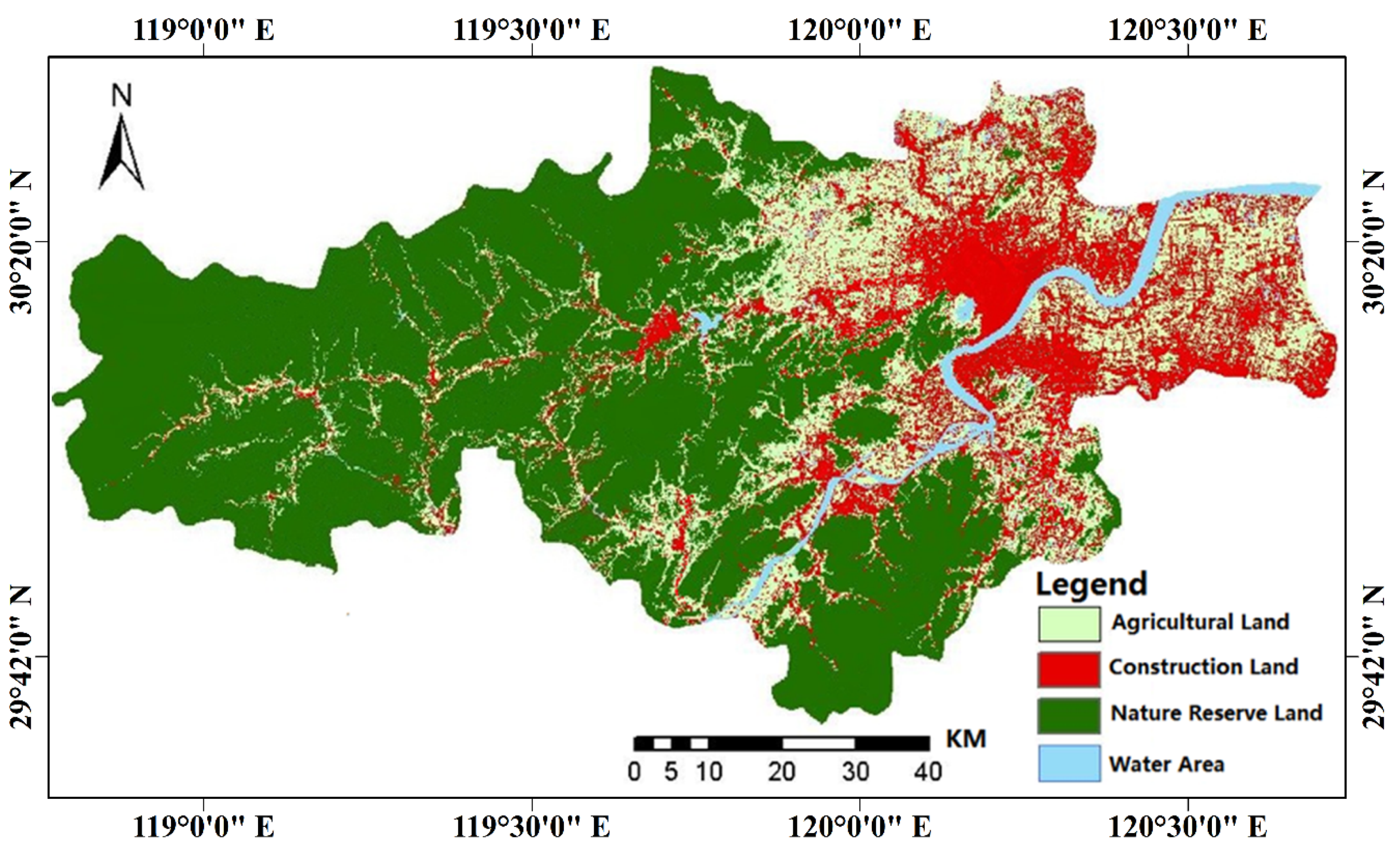
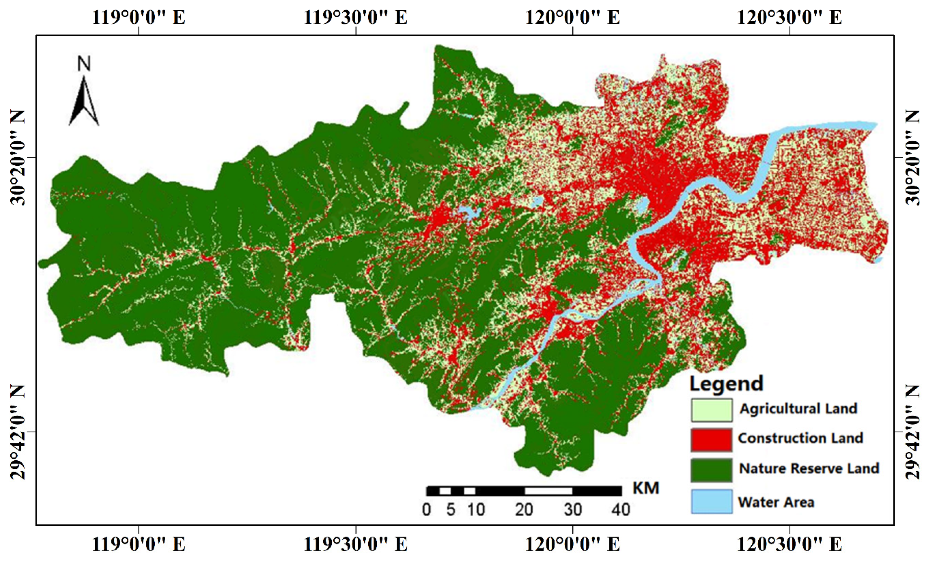
2.1. Study Area and Data

Hangzhou is located in the southeast coast of China, which is the political, economic, cultural, and financial center of Zhejiang Province. Hangzhou has a complex topography: The west is a hilly area with the main mountain range, including Tianmu Mountain, and the east is a plain area with low-lying terrain and dense river networks.

The 2006 Landsat TM and the 2013 Landsat8 remote-sensing image with 30 m resolution of the study area were downloaded from http://www.gscloud.cn/. Other experiment datasets included DEM with a 30 m resolution, road-network data, traffic-site data, and location-address data.

Nowadays, many researches develop their own auto image-identification method to classify the high-resolution image, especially unmanned aerial vehicle (UAV) images [37,38]. Because Landsat images were the medium-resolution image, we chose to use a semi-manual method to preprocessed and interpreted to obtain land-use data using ENVI 5.3 and ArcGIS 10.2. [39]. As shown in Figure 1, the workflow of Landsat images classification included four main steps, namely definition of the classification inputs, preprocessing, region of interest, and classification. The processing steps mainly included geocorrection, geometric rectification, or image registration, radiometric calibration and atmospheric correction, and topographic correction [40]. A support-vector-machine (SVM) classifier was selected for land-use classification [41].

In general, land-use types include cultivated land, forest, grassland, waters, construction land, gardens, transportation land, unused land, and swampland. In our experiment, four land-use types were defined in the training shapefile after reclassifying. The land-use-type reclassification method of construction land (B), agricultural land (A), nature reserve (N), and water area (W) are defined as shown in

Table 1. Land-use reclassifications.

Level 1.	Level 2	Definition
Construction land (B)	Land for construction (B1), land for transportation (B2)	Land for buildings and structures.
Agricultural land (A)	Cultivated land (A1), garden (A2)	Land for agricultural production.
Water area (W)	Waters (W1), swampland (W2)	River surface, lake surface, swamp.
Nature reserve (N)	Forest (N1), grassland (N2), unused land (N3)	Land with little or no human activity that did not include agricultural land, construction land, and waters.

.

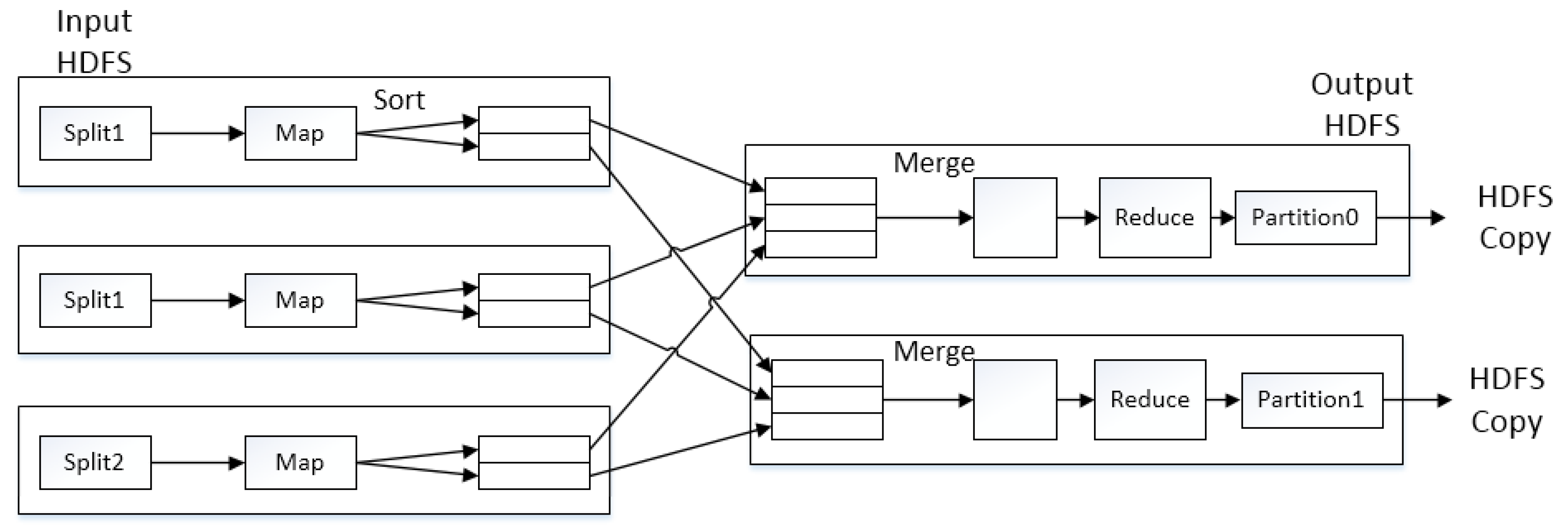
2.2. MapReduce

The MapReduce [42] program consists of two functions, Map and Reduce. Both of these functions take key/value (key-value pair) as input and output. The Map function receives a user-entered key-value pair (k₁, v₁) and processes it to generate a key-value pair (k₂, v₂) as an intermediate result. Then, the corresponding values of all the same intermediate keys (k₂) are aggregated to generate a list of values for the k₂ key list (v₂), which is used as an input to the Reduce function and processed by the Reduce function to obtain the final result list (k₃, v₃). The process can be expressed by the following formula:

$$\begin{array}{c}\mathrm{Map}:\left(k_1,v_1\right)-\mathrm{list}\left(k_2,v_2\right)\end{array}$$

(1)

$$\begin{array}{c}\mathrm{Reduce}:\left(k_2,\mathrm{list}\left(v_2\right)\right)-\mathrm{list}\left(k_3,v_3\right)\end{array}$$

(2)

The MapReduce framework is shown in Figure 2:

2.3. CA Markov Model

The Markov model is based on the theory of random processes. In this model, given the initial state and state-transition probabilities, simulation results have nothing to do with the historical condition before the current condition, which can be used to describe land-use changes from one period to another. We can also use this as a basis to predict future changes. Change was found by creating a land-use-change transition-probability matrix from periods t to t + 1, which is the basis to predict future land-use changes [43].

$$\begin{array}{c}S\left(t+1\right)=P_{ij}\times S\left(t\right)\end{array}$$

(3)

S(t + 1) denotes the state of the land-use system at times t + 1 and t, respectively. $P_{\mathrm{ij}}$ is the state-transition matrix.

CA has four basic components: Cell and cell space, cell state, neighborhood, and transition rules. The CA model can be expressed as follows [44]:

$$\begin{array}{c}S\left(t+1\right)=f\left(S\left(t\right),N\right)\end{array}$$

(4)

In the formula, S is a state set of a finite and discrete state, t and t + 1 are different moments, N is the neighborhood of the cell, and f is the cell-transition rule of the local space.

Usually, in order to make cellular automata better simulate a real environment, space constraint variable β needs to be introduced to express the topographic terrain, as well as the adaptive constraints and restrictive constraints of the spatial-influence factors on the cells. The formula becomes

$$\begin{array}{c}S\left(t+1\right)=f\left(S\left(t\right),N,\beta \right).\end{array}$$

(5)

The separate Markov model lacks spatial knowledge and does not consider the spatial distribution of geographic factors and land-use types, while the CA-Markov model adds spatial features to the Markov model, uses a cellular-automata filter to create weight factors with spatial character, and changes the state of the cells according to the state of adjacent cells and the transition rules [21].

3. Methods

3.1. Parallel CA-Markov Model Overview

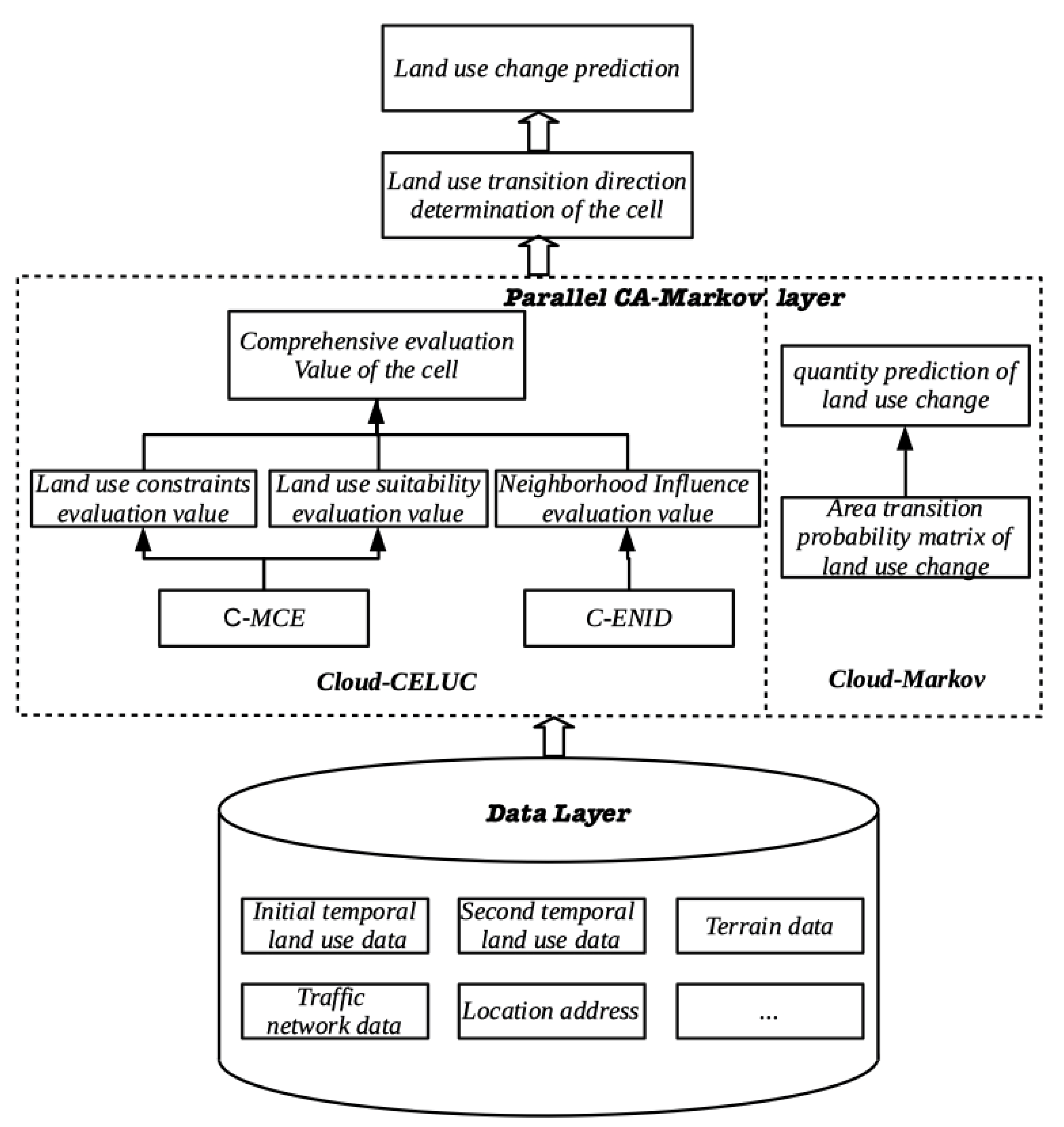
3.1.1. Parallel CA-Markov Structure

Figure 3 is the structure of parallel CA-Markov over MapReduce framework. The structure contains four layers from bottom to top: The data layer, parallel CA-Markov model layer, land-use transition-direction determination layer, and land-use prediction layer.

The experiment data include two-phase remote-sensing images, terrain data, traffic-network data, and location-address data.

The parallel CA-Markov model can mainly be divided into two parts: A parallel Markov algorithm based on MapReduce (Cloud-Markov), and a comprehensive evaluation method of land-use changes based on MapReduce (Cloud-CELUC).

Cloud-Markov was used to calculate the area transition-probability matrix of land-use changes. The algorithm of Cloud-Markov is discussed in Section 3.2.

Cloud-CELUC includes three main parts: Evaluation of the influence of neighborhoods under a cloud-computing environment (C-ENID), multicriteria evaluation under a cloud-computing environment (C-MCE), and comprehensive evaluation of land use. Among them, C-ENID is a parallel CA model over MapReduce, and C-MCE is a MapReduce algorithm to calculate constrained-evaluation and suitability-evaluation values. The cell’s neighborhood influences and C-ENID’s calculation method is discussed in Section 3.3.1. C-MCE design factors are discussed in Section 3.3.2, and the Cloud-CELUC algorithm is discussed in detail in Section 3.3.3.

After using Cloud-Markov to calculate the transition-probability matrix of land-use changes and using Cloud-CELUC to calculate each cell’s comprehensive evaluation value, each cell’s land-use transition direction was determined, which is discussed in Section 3.4. Finally, land-use-change predictions were obtained, and the land-use prediction experiment is discussed in Section 4.

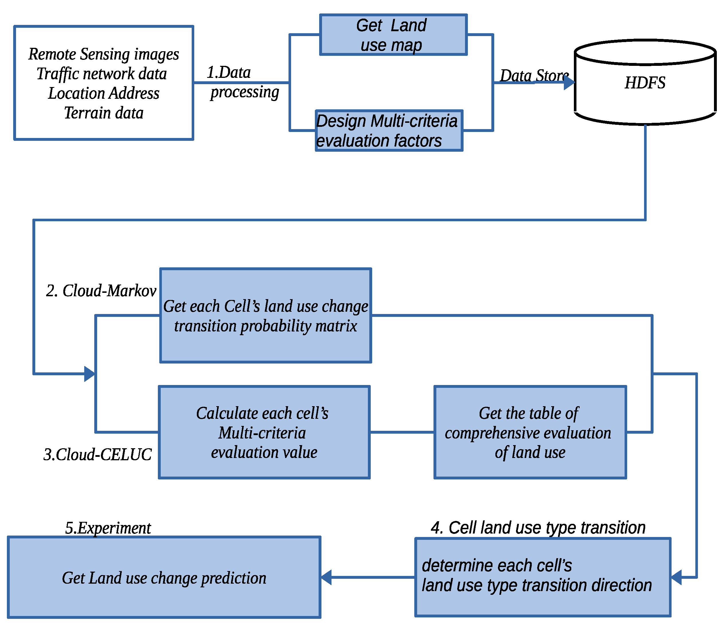
3.1.2. Parallel CA-Markov Workflow

As shown in Figure 4, the flow of the parallel CA-Markov model has five major steps, as follows:

(1)

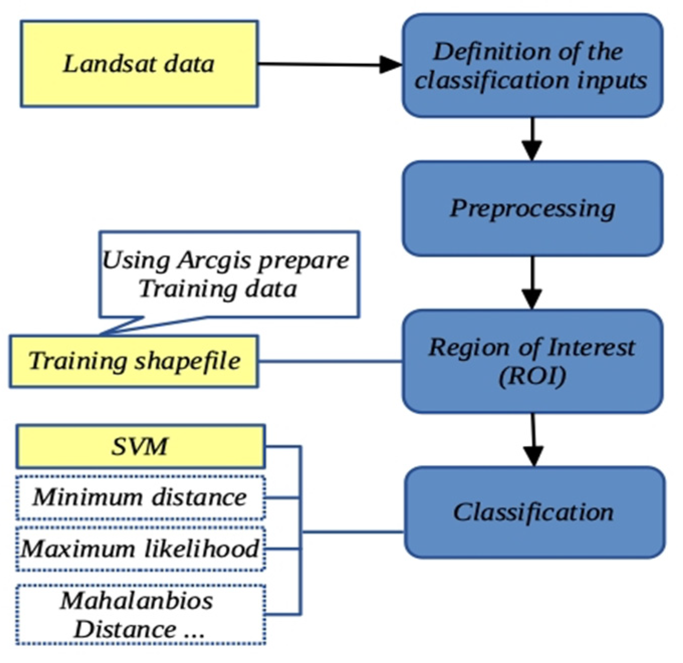
Data-processing: Preprocessing and interpreting remote-sensing images to land-use maps, designing multicriteria-evaluation factors, and storing images, land-use data, and multicriteria-evaluation factors into the Hadoop HDFS.

(2)

Parallel Markov: Using the overlay method, analyzing two-phase images and land-use data to obtain each cell’s land-use-type transition probability, and calculating the total number of cells in each land-use-type transition direction, and counting the area transition-probability matrix of each land-use type.

(3)

Parallel CA: In Cloud-CELUC, C-ENID was used to calculate the cell’s neighborhood influence value. C-MCE was designed to calculate multicriteria-evaluation values, including constraint-evaluation and suitability-evaluation values. These values were then used to calculate the statistical table of comprehensive evaluation of land use.

(4)

Transition-direction determination stage: Loop reading each cell’s transition probability from the statistical table of comprehensive-evaluation values in the parallel CA stage and combining the area transfer-probability matrix of each land-use type in the parallel Markov stage to decide a cell’s land-use-type transition direction.

(5)

Land-use-change prediction: In our experiment, we used data from 2006 to predict 2013 land-use changes and then evaluate the precision of the parallel CA-Markov model with a Kappa coefficient. Land-use change prediction for 2020 was then obtained.

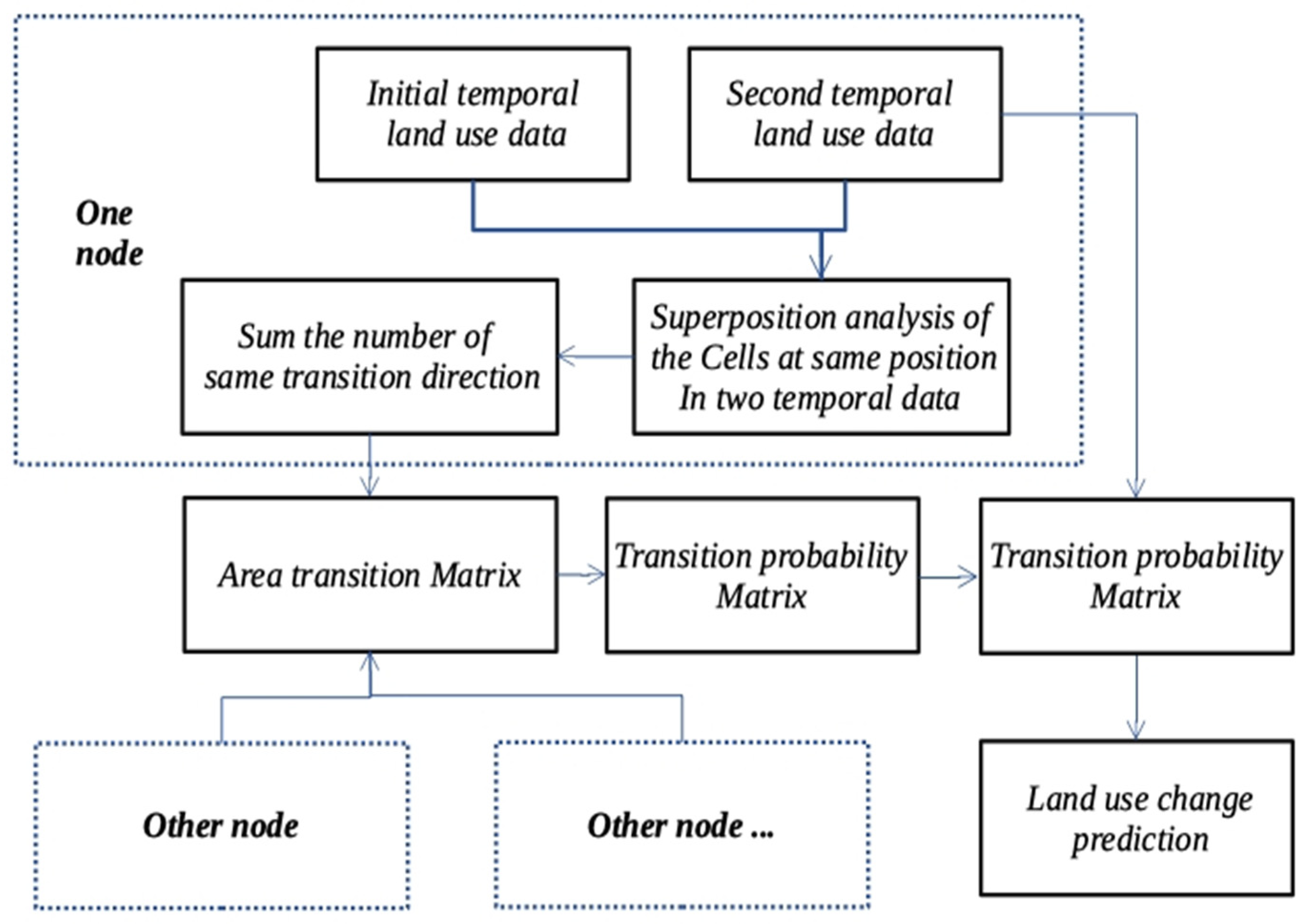
3.2. Markov Model Parallel Processing (Cloud-Markov)

Using an overlay method to analyze two-phase raster images and land-use data with the same spatial position, we obtained the transition direction of each cell and calculated the number of cells in each transition direction, then obtained the area transfer matrix of each land-use type and calculated the area probability matrix of land use. Each year’s area transfer matrix was then obtained using the probability matrix divided by the intervals of these two raster images. Then, MapReduce functions of the Markov model given in the study area are as follows:

$$\begin{array}{c}\mathrm{Map}:\left(N,\left(T_1,T_2\right)\right)\to List\left(C_{mk,}i\right)\end{array}$$

(6)

$$\begin{array}{c}\mathrm{Combiner}:M\left(C_{mk,}list\left(i\right)\right)\to List\left(C_{mk,}\mathrm{s}\right)\end{array}$$

(7)

$$\begin{array}{c}\mathrm{Reduce}:L\left(C_{mk,}list\left(i\right)\right)\to List\left(C_{mk,}\mathrm{s}\right)\end{array}$$

(8)

where N is the row offset of the input row, T₁ represents all cells’ land-use type of the earlier raster image, T₂ represents all cells’ land-use type of the later raster image, C_mk represents the cell conversion from land-use type m to land-use type k, i indicates the cell transfer number of C_mk, M is the number of land-use types in a MapReduce node, s is the total cell number of C_mk in a MapReduce node, L is the total number of land-use types, and q is the combined value of the total number of cells and transition probability for C_mk conversion in the entire study area. For example, “100-3.12%” means that there were 100 cells with C_mk conversion, and transition probability was 3.12%. Figure 5 is the flow of Cloud-Markov algorithm. After summing the number of same land-use type transition direction in each node, the area transition matrix was calculated at the Reduce stage.

The steps are as follows:

(1)

Map stage:

①

Input <Key,Value>

②

Raster cell’s land-use type conversion analysis

In this step, by comparing the cells in the same position between these two raster images, we obtained a list of C_mk. If the value of C_mk is ‘B-A’, it means that the land-use-type of the cell with the same position in different raster images is converted from B into A.

   ③

Output <Key,Value>

where key is conversion direction C_mk, and Value is an integer equal to 1.

(2)

Combiner stage:

①

Enter <Key,Value>

②

Calculate the number of each land-use-type conversion direction in each node

<Key,Value> is a key-value pair (C_mk,s), where C_mk is the conversion direction and s is the total number of cells in a MapReduce node where the C_mk land-use-type conversion direction occurs.

   ③

Output <Key,Value>

Output key-value pairs (C_mk,s).

(3)

Reduce stage:

①

Enter <Key,Value>

②

Calculate transition probability

The transition-probability-matrix calculation formula is defined as follows:

$$\begin{array}{c}{P}_{mk}=\frac{V_{mk}}{S_m}\end{array}$$

(9)

where V_mk is the value that summed C_mk from all MapReduce nodes and S_m is the number of the initial raster image’s cells whose land-use type is m.

   ③

Output <Key,Value>

<Key,Value> is a key-value pair (V_mk,P_mk), where V_mk is the land-use-type area-conversion matrix and P_mk is the transition-probability matrix.

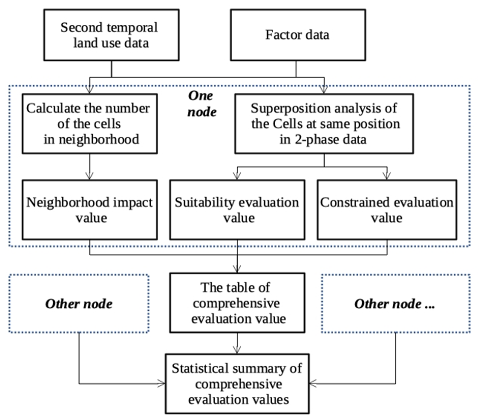
3.3. Cloud-CELUC

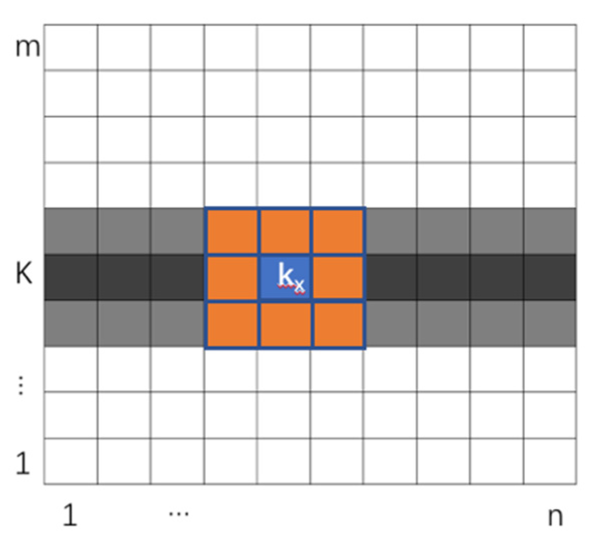
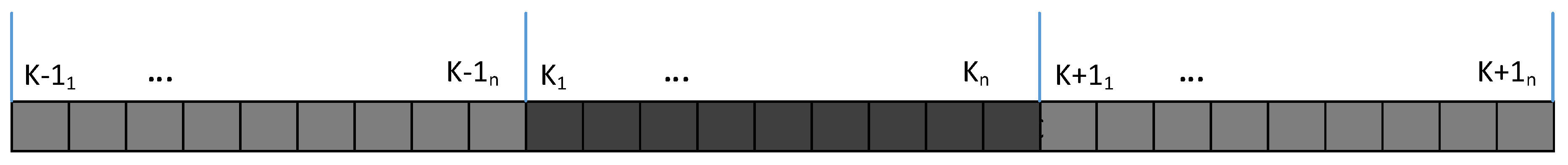
3.3.1. Cell Neighborhood Processing

Obtaining a cell’s neighborhood-influence value requires reading the state of the neighbor cells. The general neighborhood-influence evaluation methods include Von Neumann and Moore. Figure 6 shows how to read cellular-neighborhood, where we chose the $3\times 3$ Moore method to design our algorithm.

Figure 7 shows the process of cellular-dimension reduction, where a list structure was used to store all cells, so we could read each cell’s neighborhood cells through the cell’s row index and column index. The two-dimensional raster image was reduced into a one-dimensional array that could reduce the data exchange between each node during MapReduce processes. For example, the neighborhood cells of cell K_x were from line K − 1, K, and K + 1, were recorded as K − 1_x−1, K − 1_x, K − 1_x+1, K_x−1, K_x+1, K + 1_x−1, K + 1_x, and K + 1_x+1, and then stored as an array structure into the HDFS.

3.3.2. Multicriteria Evaluation Factors

This research used the multicriteria evaluation (MCE) method to calculate constraint-evaluation and suitability-evaluation values. The purpose of MCE is to select the optimal decision solution in limited (infinite) solutions between which there are conflicts and coexistence [45].

The evaluation criteria of MCE are divided into two parts: Suitable factors and constraint factors. Suitable factors are used to normalize the influencing factor to the continuous measurable values, and constraint factors are utilized to categorize spatial features by their spatial characteristics. The value of the factors is a Boolean type with a value of 0 or 1.

Suitability factors are defined and standardized in

Table 2. Suitability-factor classification.

Factor Name	Definition	Classification
FreLev	Distance from cell to highway.	Cell distance from main road or town center: 0–250, 250–500, 500–750, 750–1000, and 1000–1250 m.
TownLev	Distance from cell to town center.
SubLev	Distance from cell to subway station.	Cell distance to subway or bus station, other roads: 0–100, 100–200, 200–300, 300–400, and 400–500 m.
BusLev	Distance from cell to bus stop.
MainLev	Distance from cell to other roads.
TraLev	Distance from cell to train station.	Cell distance to train or bus station: 0–200, 200–400, 400–600, 600–800, and 800–1000 m.
StaLev	Distance from cell to bus station.
CityLev	Distance from cell to county center.	Cell distance to main road or county center: 500–1000, 1000–1500, 1500–2000, and 2000–2500 m.

, where eight factors are defined to distinguish the distance from a cell to different typical destination, and according to different land-use type, the weighted value of each factor is defined in

Table 3. Weight parameters of suitability factors.

Factor Name	Agricultural Land	Construction Land	Nature Reserve
FreLev	0.0485	0.0461	0.0781
TownLev	0.1239	0.1332	0.1010
SubLev	0.0621	0.1320	0.0133
BusLev	0.0721	0.1110	0.0513
MainLev	0.0921	0.1102	0.0749
TraLev	0.0423	0.1333	0.0201
StaLev	0.0623	0.1321	0.0203
StaLev	0.0923	0.2021	0.0103

. Then, the analytic hierarchy process (AHP) method and the expert scoring method were used to calculate the weights of the suitability factors [46], which are shown in Table 2. The waters and gradient factors were defined as the constraint factors.

The value of the constraint factors is Boolean, which is determined by land-use type. This research defined the constraint factors of hills with gradients greater than 25 degrees, and waters and ecological reserves equal to 0, because these land-use types would rarely change.

3.3.3. Parallel Cloud-CELUC Algorithm

Cloud-CELUC only needs the Map function to calculate factors and obtain comprehensive-evaluation values. The Reduce function of Cloud-CELUC was only used to output the results. The Map function was defined as follows:

$$\begin{array}{c}\mathrm{Map}:\left(N,\left(i,H_1,H_2,H_3,H_4,\dots H_m\right)\right)\to \left(\left(i,j\right),\left(L_1,L_2,L_3,\dots L_m\right)\right)\end{array}$$

(10)

where N is the line offset of the input line, i is the line index of the raster image, j is the column index of the raster image, H₁ is the cell-state value to be calculated, and H₂ and H₃ indicate the uplink and downlink cell-state values of H₁. H₄, … H_m are various constraint factors and suitability factors corresponding to the cell, and L_m is the value combined by the cell’s composite-evaluation value of the transition direction and the cell’s corresponding transition direction. For example, If L₁ is ‘ba-1.2234’, the evaluation value of the cell (i, j) from the initial land-use type ‘b’ to the final land-use type ‘a’ is ‘1.2234’.

The flow of Cloud-CELUC algorithm is shown in Figure 8, where the table of comprehensive evaluation value was obtained after each node by calculating the neighborhood impact value, suitability evaluation value, and constrained evaluation value. The steps are as follows:

①

Enter <Key,Value>

②

Calculate neighborhood-influence evaluation value (NID)

According to H₁ and H₃, the neighborhood-influence degree of each cell in H₂ was calculated. The calculation formula for the evaluation value of the neighborhood-influence degree of the cell (i,j) corresponding to a class at a certain time is as follows:

$$\begin{array}{c}NI{D}_a=\frac{1}{h-1}{\displaystyle \sum }Yes\left(S_{ij}==a\right)\end{array}$$

(11)

where h is the number of neighborhood cells, and $Yes\left(S_{ij}==a\right)$ is used to judge whether the neighbor cell’s land-use type of cell (i, j) is a or not. If a is 1, then $Yes\left(S_{ij}==a\right)$ returns 1, otherwise, it returns 0.

③

Calculate Suitability-Evaluation Value (SEV)

The calculation formula of the suitability-evaluation value is as follows:

$$\begin{array}{c}SE{V}_a={\displaystyle \sum }{V}_{a\delta }\times DI{S}_{ij\delta }\end{array}$$

(12)

where $V_{a\delta }$ is the weight of factor δ corresponding to land-use type ‘a’, $DI{S}_{ij\delta }$ are the suitability factors of cell (i,j) that are defined in Table 1.

④

Calculate constraint-evaluation value (CEV)

The constraint-evaluation formula is as follows:

$$\begin{array}{c}CE{V}_a={\displaystyle \prod }Yes\left(K_{ij}\right)\end{array}$$

(13)

where $Yes\left(K_{ij}\right)$ represents the constraint-evaluation value of cell (i, j) corresponding to constraint factor ‘k’. If the cell is constrained, $Yes\left(K_{ij}\right)$ returns 0, otherwise, it returns 1.

⑤

Calculate comprehensive-evaluation value (CELUC)

Based on the three evaluation values above, NID, SEV, and CEV, the comprehensive-evaluation formula was defined as follows:

$$\begin{array}{c}CELU{C}_a=NI{D}_a\times SE{V}_a\times CE{V}_a\end{array}$$

(14)

where a is a land-use type.

⑥

Output <Key,Value>

<Key,Value> is a key-value pair ((i, j), CELUC) where i is the cell’s row index, j is the cell’s column index, and CELUC is the comprehensive-evaluation value of the cell.

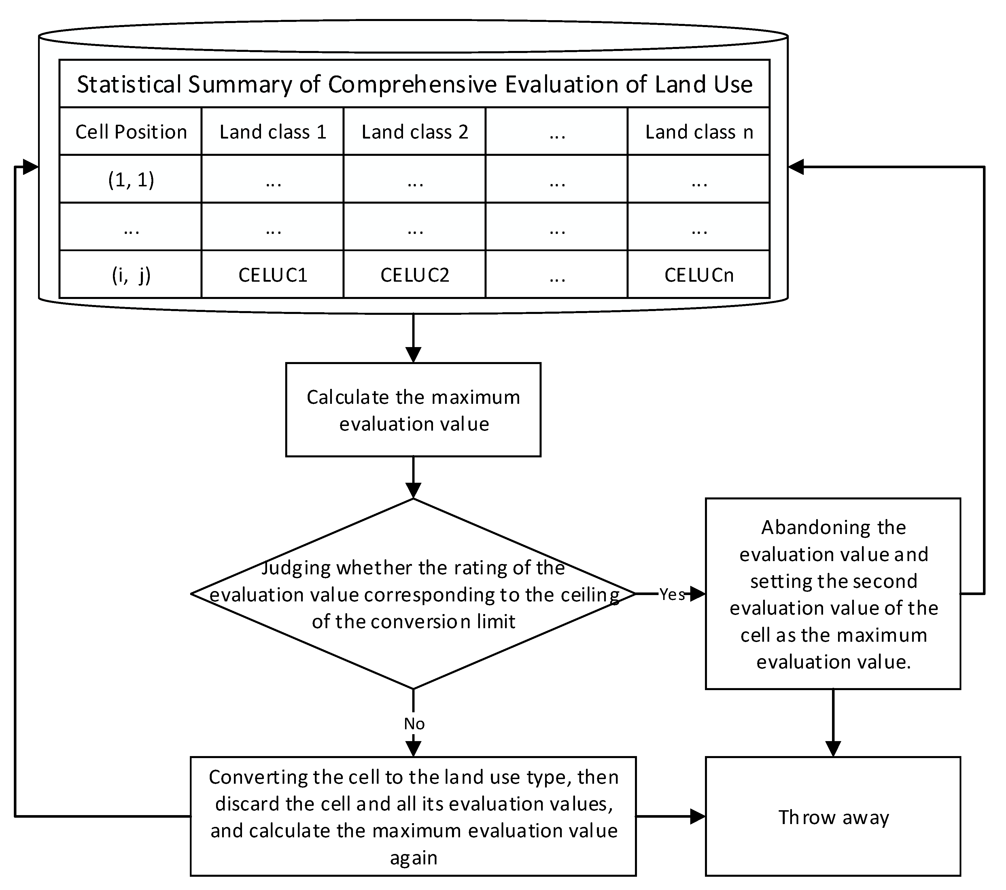
3.4. Cell Land-Use-Type Conversion

The multi-objective land-use competition method was used to achieve cells’ land-use-type conversion, which was to solve the problem when the cell had confliction in land-use-type conversion [47]. For example, if there were N types of land-use types, cell (i, j) may have had N kinds of conversion possibilities. According to constraint factors, suitability factors, and neighborhood conditions, each cell’s conversion possibility should be given a comprehensive evolution value of land use. If the evaluation value of the cell’s transition direction is determined by the biggest conversion possibility, the value may lead to a proliferation of dominant land-use types and cause oversimulation of dominant land-use types and inadequate simulation of weak land-use types. Hence, both land-use comprehensive evaluation values and the area transfer matrix of land-use changes were used to decide the cell’s conversion direction. Figure 9 shows the flow of a cell’s land-use-type conversion process.

The steps are as follows:

①

Calculating the maximum evaluation value from the table of statistical summary of comprehensive evaluation that was obtained from Cloud-CELUC.

②

Loop reading each row of the table. Each row was a key-value pair ((i, j), CELUCs), where (i, j) is the position of the cell, CELUCs means cell (i, j) has N kinds of land-use conversion possibilities (CELUC), and CELUCi means the ith CELUC of the cell.

③

Determining whether the area of the converted land-use type reached the upper area limit of this land-use-type conversion or not.

The upper area limit of the land-use-type conversion was obtained from the area transition-probability matrix of each land-use type, defined as a key-value pair (V_mk, P_mk) where V_mk is the land-use-type area conversion matrix and P_mk is the land-use transition-probability matrix at the CLOUD-Markov stage.

④

If reaching the upper area limit, the CELUCi of the cell should be marked as 0, meaning that one of the cell (i, j)’s CELUCi was deleted to make sure the CELUCi would not be used in the subsequent steps. Then, it returns to the first step.

If the upper area limit is not reached, the land-use type of the cell would be converted into a new land-use type and stored as a key-value pair ((i, j), CELUCi) into an array, discarding the other CELUCs to make sure the cell is not used in the subsequent steps. Then, it returns to the first step.

⑤

Repeating the above steps until all cells completed conversion, and finally obtaining the prediction of the whole land-use-change distribution, which was stored as an array. Each item of the array was a key-value pair ((i, j), CELUC).

4. Results and Discussion

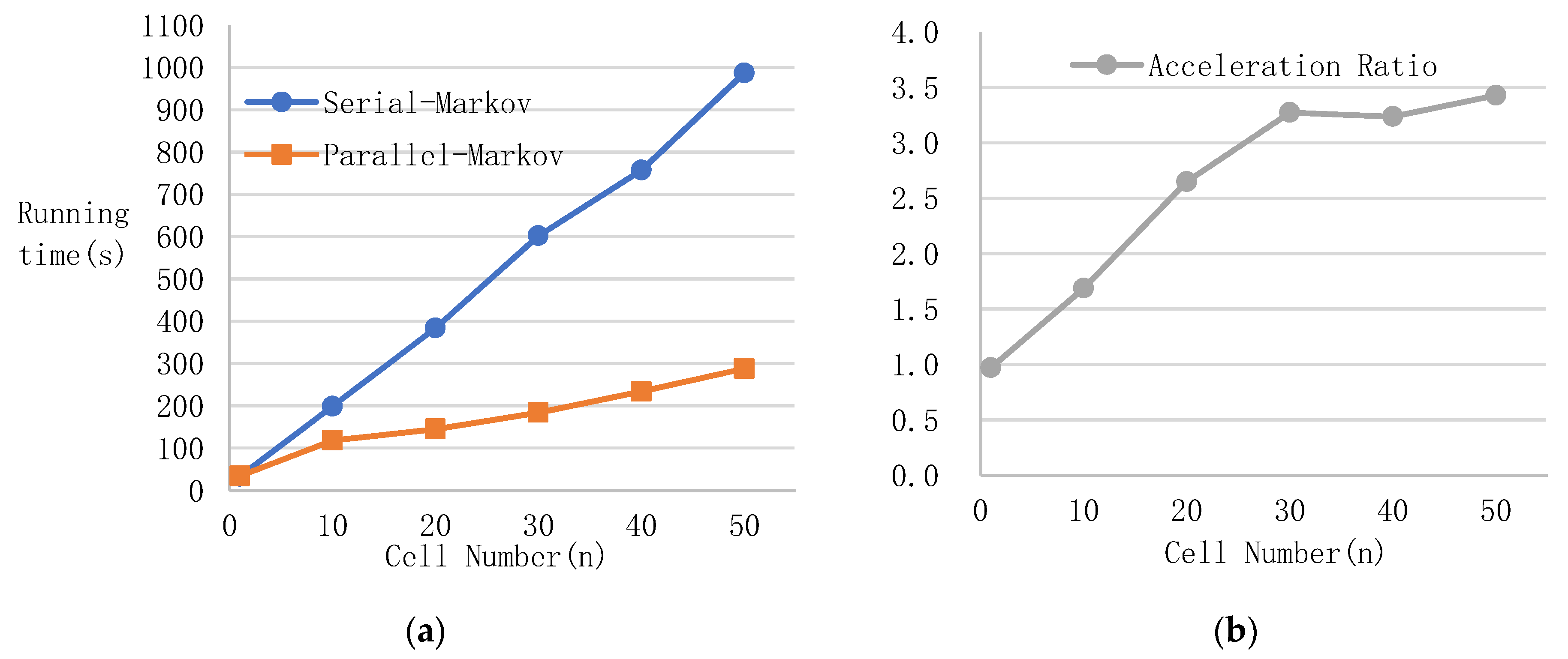
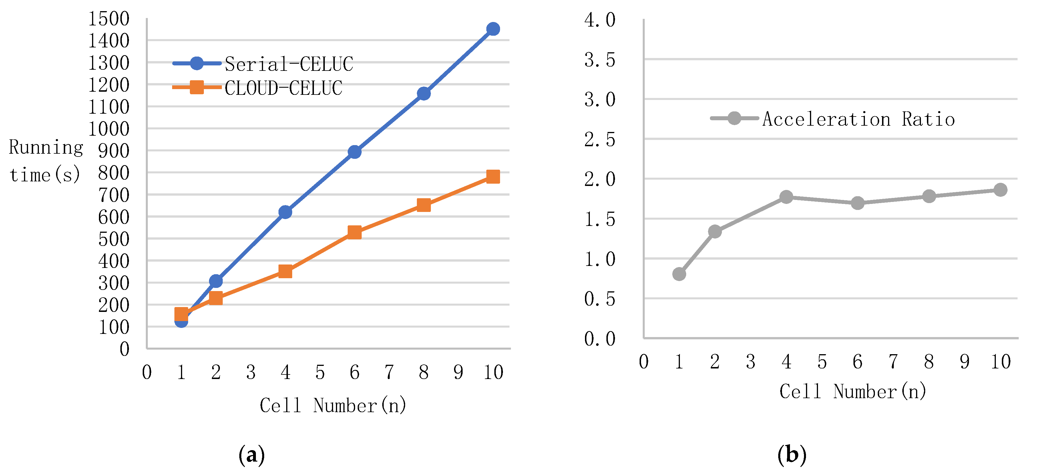
4.1. Model-Efficiency Analysis

One machine was used as the master node for the work of NameNode and JobTracker, and four other machines were used as the slave nodes for the work of DataNode and TaskTracker. The operating environment of the machines was the CentOS 7.1.1503 system with Java version 1.8.0_112 and Hadoop version 2.7.3. The experiment environment configuration is shown in

Table 4. Hadoop experiment environment.

IP Address	Node Role	CPU	RAM
192.168.128.1	Master/Namenode/Jobtracker	Four-core 2.4 Ghz	4 G
192.168.128.2	Slaves/Datanode/Tasktracker	Four-core 2.4 Ghz	4 G
192.168.128.3	Slaves/Datanode/Tasktracker	Four-core 2.4 Ghz	4 G
192.168.128.4	Slaves/Datanode/Tasktracker	Four-core 2.4 Ghz	4 G
192.168.128.5	Slaves/Datanode/Tasktracker	Four-core 2.4 Ghz	4 G

. The hardware environment of the serial algorithm was the same as the hardware of the Hadoop node.

The running efficiency and acceleration ratio results of the serial-Markov algorithm relative to Cloud-Markov algorithm are shown in Figure 10. The running efficiency and acceleration ratio results of the serial-CELUC algorithm relative to Cloud-CELUC algorithm are shown in Figure 11. As shown in Figure 10a and Figure 11a, the abscissa axis indicates the number of the cells (1 n is approximately 9,000,000) and the ordinate axis indicates running time.

The results showed that the execution time of Cloud-Markov was less than that of the serial Markov algorithm, and with the increase of input data, the acceleration ratio increased and tended to smooth. The acceleration ratio of the Cloud-Markov algorithm to the serial Markov algorithm tended to be steady at 3.27, and the acceleration ratio of Cloud-CELUC to serial CELUC tended to be steady at 1.77. The highest acceleration ratio of Cloud-Markov could reach 3.43, and the highest acceleration ratio of Cloud- CELUC could reach 1.86.

The efficiency of the parallel Markov model based on a cloud environment was remarkable because the MapReduce system effectively distributed the workload of the two phases of cell matching and quantitative statistics. The efficiency of Cloud-CELUC was also improved because the Map phase we defined ran very fast. However, when the output of the Map phase was input into the Reduce phase, it occupied a relatively large part of the long running time, which reduced the efficiency of the operation.

4.2. Precision Evaluation and Result Analysis

4.2.1. Precision Evaluation

The 2006 remote-sensing images and other data were defined as the initial data, and the 2013 land-use changes were simulated by suing the parallel CA-Markov model. In our experiment, the water area was fixed with no change. Based on the 2006 and 2013 land-use data, the area transition-probability matrix could be calculated.

Table 5. The 2006–2013 area transition matrix (unit: km²).

	2013	Agricultural Land	Construction Land	Nature Reserve	Total
2006
Agricultural land		1282.95	409.71	95.67	1788.33
Construction land		210.94	1381.69	12.52	1605.15
Nature-reserve land		93.39	50.79	4409.60	4553.78
Total		1587.28	1842.19	4517.79	7947.26

is the 2006–2013 area transition matrix, in which each cell represents the total area of one land-use type transferring to another land-use type from 2006 to 2016.

Table 6. The 2006–2013 transition-probability matrix (unit: %).

	2013	Agricultural Land	Construction Land	Nature Reserve
2006
Agricultural land		71.74	22.91	5.35
Construction land		13.14	86.08	0.78
Nature-reserve land		2.05	1.12	96.83

is the 2006–2013 transition-probability matrix, in which each cell represents the probability of one land-use type transferring to another land-use type from 2006 to 2016.

As shown in Table 5 and Table 6, the biggest land-use-type transition was agricultural land transferring to construction land; its ratio reached 22.91%. In order to evaluate the simulated precision, the 2013 land-use data were classified using real 2013 remote-sensing images at the data-processing stage. The simulated land-use data and the classified 2013 land-use data are shown in Figure 12 and Figure 13, respectively.

After simulation, the precision evaluation experiments were done to correct all kinds of weight parameters defined in C-MCE. After a great number of repetitive experiments and weight-parameter corrections, the weight parameters of the suitability factors were obtained, which are listed in Table 2. At present, commonly used precision evaluation methods include visual comparison, dimensionality tests, pixel contrasts, and the Kappa coefficient test.

With visual comparison, it was found that the simulation of the nature reserve in the western and southern regions was the most accurate. It can be concluded that the suitability factor and the constrained factor were in line with the change trend of the nature reserve in the study area. The construction land of the central urban area had better simulation accuracy. However, the construction land of east and north, including the towns of Yuanpu and Linpu, was scattered and intertwined with agricultural land. Therefore, simulation error was relatively large.

The Kappa coefficient test is the most commonly used quantitative test method [48]. When the Kappa coefficient is used to compare the consistency of data, commonly used criteria are as follows: If the two land-use maps are identical, then Kappa = 1; when Kappa > 0.8, consistency is almost perfect; when 0.6 < Kappa ≤ 0.8, consistency is substantial; when 0.4 < Kappa ≤ 0.6, consistency is moderate; when 0.2 < Kappa ≤ 0.4, consistency is slight; when 0 < Kappa ≤ 0.2, consistency is poor [49,50]. Simulated land-use data and actual classified land-use data of 2013 were compared, and the results of the Kappa coefficient are shown in

Table 7. Kappa coefficient test table of nature reserve land in 2013 (unit: km²).

	Simulated Data	Nature Reserve	Non-Nature Reserve	Total	Accuracy	Kappa
Classified Data
Nature-reserve land		4221.35	288.47	4509.82	93.60%	0.86
Non-nature-reserve land		296.44	3431.50	3727.94	92.05%
Total		4517.79	3717.97

,

Table 8. Kappa coefficient of construction land in 2013 (unit: km²).

	Simulated Data	Construction Land	Non-Construction Land	Total	Accuracy	Kappa
Classified Data
Construction land		1391.41	452.77	1844.18	75.45%	0.68
Non-construction land		450.78	5942.80	6393.58	92.95%
Total		1842.19	6395.57

and

Table 9. Kappa coefficient of agricultural land in 2013 (unit: km²).

	Simulated Data	Agricultural Land	Non-Agricultural Land	Total	Accuracy	Kappa
Classified Data
Agricultural land		1152.64	427.17	1579.81	72.96%	0. 66
Non-agricultural land		434.65	6223.30	6657.95	93.47%
Total		1587.29	6650.47

, respectively.

Results showed that the Kappa coefficients for nature reserve, construction land, and agricultural land were 0.85, 0.6, and 0.65, respectively. This meant that the 2013 results of the simulation were quite accurate [38,51,52,53], and that using the parallel CA-Markov model to predict future land use would be highly reliable.

4.2.2. Land-Use-Change Prediction

Based on the classified 2013 land-use data and other experiment data, 2020 land-use changes were predicted using the parallel CA-Markov model. The results of the 2013–2020 area transition matrix are shown in

Table 10. The 2013–2020 area transition matrix (unit: km²).

	2020	Agricultural Land	Construction Land	Nature Reserve	Total
2013
Agricultural land		1133.35	361.94	84.52	1579.81
Construction land		242.35	1587.45	14.38	1844.18
Nature-reserve land		92.49	50.30	4367.03	4509.82
Total		1468.19	1999.69	4465.93	7933.81

, and the 2020 land-use prediction map is shown in Figure 14.

As can be seen from the 2020 land-use prediction map, construction land in the study area was on the rise as a whole, and this increase mainly came from the conversion of agricultural land. Agricultural land showed a downward trend, and natural-reserve land changed little in proportion to its vast size.

The overall growth of construction land was relatively large. In particular, due to expanding road and public-transport systems, construction land grew faster in the urban center of each county. The growth of construction land in the districts of Xihu, Gongshu, Xiacheng, Binjiang, and Xiaoshan was prominent. Due to the terrain and water-body restrictions, other counties and urban areas maintained stable acreage of construction land.

Agricultural land and construction land intertwined in large areas in the northwest and north of the study area. However, the evaluation value of construction land in this area was not high because it was far from the city center and the county center and the public transportation system was less developed. The acreage of agricultural land in the above area was basically stable. The agricultural land in the rest of the study area was affected by urban expansion, the road, and public transportation systems, and large acreage was converted to construction land.

Nature reserves were mostly found in the western and southern hilly areas, which were subject to various restraints for development, such as sloping terrain and ecological-protection restrictions, and an inconvenient transportation system, and therefore remained basically stable in acreage.

5. Conclusions

Experiments showed that the results of land-use simulation based on the CA-Markov model under a cloud environment were reliable, reflecting that the method proposed in this study was reliable and applicable. Meanwhile, MapReduce was effective in parallelizing the CA-Markov model to improve the processing speed of land-use-change prediction based on the CA-Markov model. This method parallelized the CA-Markov model in two parts: The parallel Markov model based on a cloud environment (Cloud-Markov), and the comprehensive evaluation method of land-use changes based on MapReduce (Cloud-CELUC). By selecting Hangzhou as the study area and setting up a Hadoop experiment environment, the experiments were designed to verify the reliability, precision, and operating efficiency of the method. Land-use changes in Hangzhou in 2020 were simulated and the results were analyzed. The experimental results showed that the method which simultaneously realized the integrity and segmentation for land use change simulation and prediction is also practical and effective.

This research has successfully applied the MapReduce framework to improve land-use-change prediction efficiency. However, there are still some important issues worth further investigation. First, land-use changes were restrained not only by natural conditions, but also by political, economic, demographic, and other complex factors. Due to limited data sources, this study built its model mainly on traffic, terrain, and location factors. If more data are available, the prediction module of the spatial pattern of land-use, social, economic, policy, demographic, and other factors should be taken into account in future research. We will also consider combining the auto image-identification method [37] into our current work to reduce manual preprocessing work. When Cloud-CELUC acquired the output result of the Map stage in the Reduce stage, input/output (IO) became a bottleneck in system performance. Therefore, more research efforts should be dedicated to testing increasing IO efficiency on the performance of cloud computing based on the CA-Markov model.

References

- Veldkamp, A.; Lambin, E. Predicting land-use change. Agric. Ecosyst. Environ. 2001, 85, 1–6. [Google Scholar] [CrossRef]
- Li, X. A review of the international researches on land use/land cover change. ACTA Geogr. Sin. Ed. 1996, 51, 558–565. [Google Scholar]
- Wijesekara, G.N.; Farjad, B.; Gupta, A.; Qiao, Y.; Delaney, P.; Marceau, D.J. A comprehensive land-use/hydrological modeling system for scenario simulations in the Elbow River watershed, Alberta, Canada. Environ. Manag. 2014, 53, 357–381. [Google Scholar] [CrossRef] [PubMed]
- Verburg, P.H.; Soepboer, W.; Veldkamp, A.; Limpiada, R.; Espaldon, V.; Mastura, S.S.A. Modeling the spatial dynamics of regional land use: The CLUE-S model. Environ. Manag. 2002, 30, 391–405. [Google Scholar] [CrossRef] [PubMed]
- White, R.; Engelen, G. Cellular Automata and Fractal Urban Form: A Cellular Modelling Approach to the Evolution of Urban Land-Use Patterns. Environ. Plan. A Econ. Spec. 1993, 25, 1175–1199. [Google Scholar] [CrossRef] [Green Version]
- Clarke, K.C.; Hoppen, S.; Gaydos, L. A self-modifying cellular automaton model of historical urbanization in the San Francisco Bay area. Environ. Plan. B Plan. Des. 1997, 24, 247–261. [Google Scholar] [CrossRef] [Green Version]
- Zhang, C.; Li, W. Markov chain modeling of multinomial land-cover classes. GISci. Remote Sens. 2005, 42, 1–18. [Google Scholar] [CrossRef]
- Fu, X.; Wang, X.; Yang, Y.J. Deriving suitability factors for CA-Markov land use simulation model based on local historical data. J. Environ. Manag. 2018, 206, 10–19. [Google Scholar]
- Jantz, C.A.; Goetz, S.J.; Shelley, M.K. Using the SLEUTH urban growth model to simulate the impacts of future policy scenarios on urban land use in the Baltimore-Washington metropolitan area. Environ. Plan. B Plan. Des. 2004, 31, 251–271. [Google Scholar] [CrossRef]
- Dietzel, C.; Clarke, K.C. Toward optimal calibration of the SLEUTH land use change model. Trans. GIS 2007, 11, 29–45. [Google Scholar] [CrossRef]
- Serneels, S.; Lambin, E.F. Proximate causes of land-use change in Narok district, Kenya: A spatial statistical model. Agric. Ecosyst. Environ. 2001, 85, 65–81. [Google Scholar] [CrossRef]
- Wolfram, S. Cellular automata as models of complexity. Nature 1984, 311, 419–424. [Google Scholar] [CrossRef]
- Batty, M.; Xie, Y.; Sun, Z. Modeling urban dynamics through GIS-based cellular automata. Comput. Environ. Urban Syst. 1999, 23, 205–233. [Google Scholar] [CrossRef] [Green Version]
- Li, X.; Yeh, A.G.-O. Neural-network-based cellular automata for simulating multiple land use changes using GIS. Int. J. Geogr. Inf. Sci. 2002, 16, 323–343. [Google Scholar] [CrossRef]
- Yang, Q.; Li, X.; Shi, X. Cellular automata for simulating land use changes based on support vector machines. Comput. Geosci. 2008, 34, 592–602. [Google Scholar] [CrossRef]
- Yang, X.; Zheng, X.-Q.; Lv, L.-N. A spatiotemporal model of land use change based on ant colony optimization, Markov chain and cellular automata. Ecol. Model. 2012, 233, 11–19. [Google Scholar] [CrossRef]
- Rimal, B.; Zhang, L.; Keshtkar, H.; Wang, N.; Lin, Y. Monitoring and Modeling of Spatiotemporal Urban Expansion and Land-Use/Land-Cover Change Using Integrated Markov Chain Cellular Automata Model. ISPRS Int. J. Geo. Inf. 2017, 6, 288. [Google Scholar] [CrossRef]
- Subedi, P.; Subedi, K.; Thapa, B. Application of a Hybrid Cellular Automaton—Markov (CA-Markov) Model in Land-Use Change Prediction: A Case Study of Saddle Creek Drainage Basin, Florida. Appl. Ecol. Environ. Sci. 2013, 1, 126–132. [Google Scholar]
- Bacani, V.M.; Sakamoto, A.Y.; Quénol, H.; Vannier, C.; Corgne, S. Markov chains-cellular automata modeling and multicriteria analysis of land cover change in the Lower Nhecolândia subregion of the Brazilian Pantanal wetland. J. Appl. Remote Sens. 2016, 10, 016004. [Google Scholar] [CrossRef]
- Araya, Y.H.; Cabral, P. Analysis and modeling of urban land cover change in Setúbal and Sesimbra, Portugal. Remote Sens. 2010, 2, 1549–1563. [Google Scholar] [CrossRef]
- Halmy, M.W.A.; Gessler, P.E.; Hicke, J.A.; Salem, B.B. Land use/land cover change detection and prediction in the north-western coastal desert of Egypt using Markov-CA. Appl. Geogr. 2015, 63, 101–112. [Google Scholar] [CrossRef]
- Hishe, S.; Bewket, W.; Nyssen, J.; Lyimo, J. Analysing past land use land cover change and CA-Markov-based future modelling in the Middle Suluh Valley, Northern Ethiopia. Geocarto Int. 2019, 1–31. [Google Scholar] [CrossRef]
- Rahman, M.T.U.; Tabassum, F.; Rasheduzzaman, M.; Saba, H.; Sarkar, L.; Ferdous, J.; Uddin, S.Z.; Islam, A.Z.M.Z. Temporal dynamics of land use/land cover change and its prediction using CA-ANN model for southwestern coastal Bangladesh. Environ. Monit. Assess. 2017, 189, 565. [Google Scholar] [CrossRef] [PubMed]
- Memarian, H.; Kumar Balasundram, S.; Bin Talib, J.; Teh Boon Sung, C.; Mohd Sood, A.; Abbaspour, K. Validation of CA-Markov for Simulation of Land Use and Cover Change in the Langat Basin, Malaysia. J. Geogr. Inf. Syst. 2012, 4, 542–554. [Google Scholar] [CrossRef] [Green Version]
- Liang, J.; Zhong, M.; Zeng, G.; Chen, G.; Hua, S.; Li, X.; Yuan, Y.; Wu, H.; Gao, X. Risk management for optimal land use planning integrating ecosystem services values: A case study in Changsha, Middle China. Sci. Total Environ. 2017, 579, 1675–1682. [Google Scholar] [CrossRef] [PubMed]
- Liu, X.H.; Andersson, C. Assessing the impact of temporal dynamics on land-use change modeling. Comput. Environ. Urban Syst. 2004, 28, 107–124. [Google Scholar] [CrossRef]
- Mobaied, S.; Riera, B.; Lalanne, A.; Baguette, M.; Machon, N. The use of diachronic spatial approaches and predictive modelling to study the vegetation dynamics of a managed heathland. Biodivers. Conserv. 2011, 20, 73–88. [Google Scholar] [CrossRef]
- Alsharif, A.A.A.; Pradhan, B. Urban Sprawl Analysis of Tripoli Metropolitan City (Libya) Using Remote Sensing Data and Multivariate Logistic Regression Model. J. Indian Soc. Remote Sens. 2014, 42, 149–163. [Google Scholar] [CrossRef]
- Guan, Q.; Clarke, K.C. A general-purpose parallel raster processing programming library test application using a geographic cellular automata model. Int. J. Geogr. Inf. Sci. 2010, 24, 695–722. [Google Scholar] [CrossRef] [Green Version]
- Li, X.; Zhang, X.; Yeh, A.; Liu, X. Parallel cellular automata for large-scale urban simulation using load-balancing techniques. Int. J. Geogr. Inf. Sci. 2010, 24, 803–820. [Google Scholar] [CrossRef]
- Li, D.; Li, X.; Liu, X.P.; Chen, Y.M.; Li, S.Y.; Liu, K.; Qiao, J.G.; Zheng, Y.Z.; Zhang, Y.H.; Lao, C.H. GPU-CA model for large-scale land-use change simulation. Chin. Sci. Bull. 2012, 57, 2442–2452. [Google Scholar] [CrossRef] [Green Version]
- Guan, Q.; Shi, X.; Huang, M.; Lai, C. A hybrid parallel cellular automata model for urban growth simulation over GPU/CPU heterogeneous architectures. Int. J. Geogr. Inf. Sci. 2016, 30, 494–514. [Google Scholar] [CrossRef]
- Rathore, M.M.U.; Paul, A.; Ahmad, A.; Chen, B.; Huang, B.; Ji, W. Real-Time Big Data Analytical Architecture for Remote Sensing Application. IEEE J. Sel. Top. Appl. Earth Obs. Remote Sens. 2015, 8, 4610–4621. [Google Scholar] [CrossRef]
- Rao, J.; Wu, B.; Dong, Y.-X. Parallel Link Prediction in Complex Network Using MapReduce. J. Softw. 2014, 23, 3175–3186. [Google Scholar] [CrossRef]
- Wiley, K.; Connolly, A. Astronomical image processing with hadoop. Astron. Data Anal. Softw. Syst. 2010, 442, 93–96. [Google Scholar]
- Almeer, M.H. Cloud Hadoop Map Reduce For Remote Sensing Image Analysis. J. Emerg. Trends Comput. Inf. Sci. 2012, 3, 637–644. [Google Scholar]
- Dang, L.M.; Ibrahim Hassan, S.; Suhyeon, I.; Sangaiah, A.K.; Mehmood, I.; Rho, S.; Seo, S.; Moon, H. UAV based wilt detection system via convolutional neural networks. Sustain. Comput. Inform. Syst. 2018, in press. [Google Scholar] [CrossRef]
- Sankey, T.T.; McVay, J.; Swetnam, T.L.; McClaran, M.P.; Heilman, P.; Nichols, M. UAV hyperspectral and lidar data and their fusion for arid and semi-arid land vegetation monitoring. Remote Sens. Ecol. Conserv. 2018, 4, 20–33. [Google Scholar] [CrossRef]
- Lanorte, A.; De Santis, F.; Nolè, G.; Blanco, I.; Loisi, R.V.; Schettini, E.; Vox, G. Agricultural plastic waste spatial estimation by Landsat 8 satellite images. Comput. Electron. Agric. 2017, 141, 35–45. [Google Scholar] [CrossRef]
- Du, Z.; Li, W.; Zhou, D.; Tian, L.; Ling, F.; Wang, H.; Gui, Y.; Sun, B. Analysis of Landsat-8 OLI imagery for land surface water mapping. Remote Sens. Lett. 2014, 5, 672–681. [Google Scholar] [CrossRef]
- Jia, K.; Wei, X.; Gu, X.; Yao, Y.; Xie, X.; Li, B. Land cover classification using Landsat 8 Operational Land Imager data in Beijing, China. Geocarto Int. 2014, 29, 941–951. [Google Scholar] [CrossRef]
- Dean, J.; Ghemawat, S. MapReduce. Commun. ACM 2008, 51, 107. [Google Scholar] [CrossRef]
- Guan, D.; Gao, W.; Watari, K.; Fukahori, H. Land use change of Kitakyushu based on landscape ecology and Markov model. J. Geogr. Sci. 2008, 18, 455–468. [Google Scholar] [CrossRef]
- White, R.; Engelen, G.; Uljee, I. The use of constrained cellular automata for high-resolution modelling of urban land-use dynamics. Environ. Plan. B Plan. Des. 1997, 24, 323–343. [Google Scholar] [CrossRef]
- CARVER, S.J. Integrating multi-criteria evaluation with geographical information systems. Int. J. Geogr. Inf. Syst. 1991, 5, 321–339. [Google Scholar] [CrossRef] [Green Version]
- Saaty, T.L.; Vargas, L.G. Models, Methods, Concepts & Applications of the Analytic Hierarchy Process; Springer Science & Business Media: New York, NY, USA, 2001; ISBN 978-1-4613-5667-7. [Google Scholar]
- Qiu, B.; Chen, C. Land use change simulation model based on MCDM and CA and its application. Acta Geogr. Sin. Ed. 2008, 63, 165–174. [Google Scholar]
- Foody, G.M. Map comparison in GIS. Prog. Phys. Geogr. 2007, 31, 439–445. [Google Scholar] [CrossRef]
- Landis, J.R.; Koch, G.G. The Measurement of Observer Agreement for Categorical Data. Biometrics 1977, 33, 159. [Google Scholar] [CrossRef] [Green Version]
- Viera, A.J.; Garrett, J.M. Understanding interobserver agreement: The kappa statistic. Fam. Med. 2005, 37, 360–363. [Google Scholar]
- van Vliet, J.; Bregt, A.K.; Hagen-Zanker, A. Revisiting Kappa to account for change in the accuracy assessment of land-use change models. Ecol. Model. 2011, 222, 1367–1375. [Google Scholar] [CrossRef]
- Bu, R.C.; Chang, Y.; Hu, Y.M.; Li, X.Z.; He, H.S. Measuring spatial information changes using Kappa coefficients: A case study of the city groups in central Liaoning province. Acta Ecol. Sin. 2005, 205, 4. [Google Scholar]
- Mora, A.D.; Vieira, P.M.; Manivannan, A.; Fonseca, J.M. Automated drusen detection in retinal images using analytical modelling algorithms. Biomed. Eng. Online 2011, 10, 59. [Google Scholar] [CrossRef] [PubMed]