Optimizing Wireless Sensor Network Installations by Visibility Analysis on 3D Point Clouds

Abstract

In this paper, a MATLAB tool for the automatic detection of the best locations to install a wireless sensor network (WSN) is presented. The implemented code works directly on high-resolution 3D point clouds and aims to help in positioning sensors that are part of a network requiring inter-visibility, namely, a clear line of sight (LOS). Indeed, with the development of LiDAR and Structure from Motion technologies, there is an opportunity to directly use 3D point cloud data to perform visibility analyses. By doing so, many disadvantages of traditional modelling and analysis methods can be bypassed. The algorithm points out the optimal deployment of devices following mainly two criteria: inter-visibility (using a modified version of the Hidden Point Removal operator) and inter-distance. Furthermore, an option to prioritize significant areas is provided. The proposed method was first validated on an artificial 3D model, and then on a landslide 3D point cloud acquired from terrestrial laser scanning for the real positioning of an ultrawide-band WSN already installed in 2016. The comparison between collected data and data acquired by the WSN installed following traditional patterns has demonstrated its ability for the optimal deployment of a WSN requiring inter-visibility.

1. Introduction

A wide variety of techniques aimed at monitoring the surface displacements of unstable slopes exist today. This reflects the need to assess the dynamics and possible evolution of landslides threatening vulnerable communities and infrastructures, so as to define appropriate remediation and early warning strategies [1]. Without getting into the details of all the currently available monitoring techniques, one of the most notable advancements was arguably produced by the development of ground-based and satellite radar interferometry [2]. However, devices offering extremely high accuracy and spatial coverage are typically associated with significant costs and a number of logistical constraints. For this reason, it is also important to refine practices and analysis methodologies related to monitoring techniques characterized by lower costs and higher flexibility, whose employment may be much more sustainable and equally efficient in certain scenario types. Some examples of this kind were provided by Dou et al. [3], Hemalatha et al. [4], Kromer et al. [5], and Prabha et al. [6].

In this framework, wireless sensor networks (WSNs) have recently attracted particular interest. These are defined as networks of usually low-size and low-cost devices denoted as nodes that are integrated with sensors that can gather information through wireless links [7]. Their use presents several advantages over traditional monitoring techniques, such as the capability to work in rough and hardly accessible terrain, thanks to the absence of wired structures [8]; the possibility to analyze data from a multipoint perspective [9]; the ease and speed of installation [10]; and the adaptability of sensors to be integrated with existing monitoring techniques [11,12]. To make the most out of a WSN, optimal sensor deployment (i.e., equal and thoughtful distribution) is essential, and, to this aim, sensor-deployment problems were studied in several contexts [13]. For instance, Wang et al. [14] geometrically analyzed the relationship between coverage and connectivity in a WSN considering an obstacle-free environment, and Zou and Chakrabarty [15] proposed a virtual force algorithm as a sensor-deployment strategy after an initial random placement of sensors. For some types of sensors, line of sight (LOS) cannot be neglected. Information is in fact properly transmitted if the transmitter and receiver stations are in view of each other without any obstacle. The LOS of each emitting sensor is therefore an important issue to consider when positioning two or more receivers.

Researchers are increasingly focusing on LOS-based WSNs that use the same signal both for communication and ranging purposes, allowing the relative distance between nodes to be detected and landslide deformation to be assessed [16,17,18,19]. Depending mainly on their wavelength and the characteristics of the material to cross, waves can follow several types of behavior, and problems connected to unfavorable LOS may lead to the absence of data or inaccurate measurements due to a delay in arrival time or to multiple-reflection effects [20,21,22,23]. While several existing monitoring techniques work in LOS conditions (e.g., LiDAR [24,25], GB-InSAR [26], robotic total station [27]), this issue becomes more complicated when considering WSNs, as each node has to be in LOS with the others in order to ensure complete inter-visibility for the whole network. In this context, Intrieri et al. [28] tested a WSN named Wireless sensor network for Ground Instability Monitoring (Wi-GIM), which exploits ultrawide-band signals to evaluate ranging between nodes by means of the time of arrival. It was demonstrated how non-LOS conditions (mainly due to vegetation) could cause a delay in the signal and, consequently, errors in distance evaluation, as well as data loss, hence compromising the reliability of the monitoring system. For these reasons, inter-visibility analysis is essential to correctly place and install a LOS-based WSN.

Visibility analysis is a common issue in the fields of urban design, landscape planning, and geographic information system (GIS) technologies, and most solutions are based on the use of gridded digital terrain and elevation models [29,30]. With the development of LiDAR and Structure from Motion techniques, there is now an opportunity to directly use 3D point cloud data to perform visibility analyses. Doing so, many disadvantages of traditional modelling and analysis methods can be bypassed. For example, this makes it possible to avoid the generation of a surface model that is potentially associated with a number of errors and approximations [31,32,33,34]. Furthermore, point cloud data can provide much more detailed information than traditional gridded raster-terrain data or triangulated mesh-terrain data, especially on steep, hummocky, vegetated, and/or highly irregular terrain.

In this paper, an algorithm able to find optimal locations to install sensors, part of a LOS-based WSN, is presented. This was attained by following three criteria: (i) inter-visibility between sensors was guaranteed by exploiting a modified version of the Hidden Point Removal operator by Katz et al. [33]; (ii) equal distribution of devices was ensured; and (iii) different weights were preferentially assigned to critical portions of the investigated landslide (e.g., areas more at risk, areas showing higher displacement rates, and easily accessible or stable areas). To check the reliability of the proposed algorithm, it was applied to two different datasets. The first set corresponded to a complex artificial scene representing a room with scattered vertical obstacles in the form of beams and sections of walls designed in AutoCAD 3D (Autodesk, v. 20.0) and transformed into a 3D point cloud with CloudCompare (v. 2.10). This was a challenging scene because of the difficulty of finding lines of sight in crowded obstacle scenes. In addition, obstacles with simple shapes made the scene easy to visually interpret, making it a good first example to understanding the functioning of the code. The second dataset corresponded to a real site, namely, the Roncovetro landslide, located in the Emilia Romagna Region, Central Italy. At the same site, a first monitoring campaign with the system was carried out in 2016 by Intrieri et al. [28]. It was then possible to compare the data acquired in the two campaigns and evaluate the performance of the proposed method in a real serviceable case. The final aim of this work was to quantify the improvement that the introduced method produces in a wireless sensor network, requiring free LOS.

2. Proposed Method

This paper proposes an algorithm called Wireless Sensor network Installation Optimizer (WiSIO) to geometrically find the best locations to install a WSN requiring visibility, i.e., the i^th Point (P_i). To pursue this goal, WiSIO was implemented in MATLAB (R2018a) as simple, fast, and easy code. It can be applied to several natural scenarios, such as vertical cliffs, gentle and steep slopes, and terraces. Its employment can also be extended to buildings, small objects, and, more generally, to every artificial structure without geometrical or size limits.

The central point of the algorithm is visibility analysis. Similar analyses are the common function of most geographic information system software, but, in all cases, they are based on the digital elevation model. This kind of analysis uses the elevation of each cell of the model to detect if they are visible or not from a given point of view. Line of sight from the point of view to the target cells is substantially planned, and when cells of higher elevation intersect them, the view is considered obstructed. It goes without saying that the method works well when dealing with straight lines, as is the case of buildings and roads, and this is why these viewshed analyses are usually made on the digital elevation model and not on the digital surface model. Dealing with vegetation, in fact, constrains these methods to significant geometrical approximations, even when models have good resolution. With the aim of keeping all original information, the input data of the proposed algorithm are high-resolution 3D point clouds. Working directly with point clouds, as in the case of WiSIO, aims to be able to work with harsh environments, including not only vegetation but also steep, rough, and overhanging terrain. The algorithm works without reconstructing any kind of surface, avoiding errors and approximations usually caused by traditional modelling. The heterogeneity and the resolution of 3D point clouds are consequently main limitations of the developed code: The lower the resolution of the input data is, the less reliable the output is. In this regard, input data should be a cloud obtained by merging data acquired from different positions to avoid shadow areas and to have regular distribution of points in space.

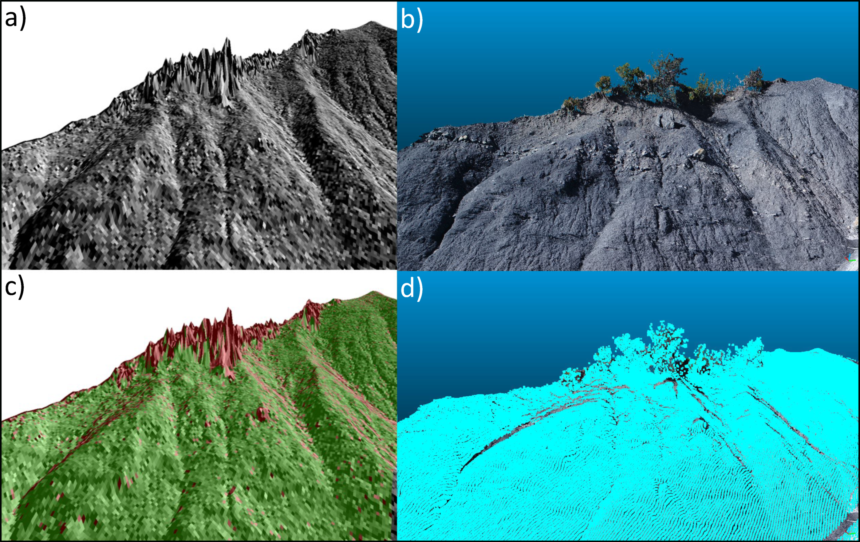
To appreciate the importance of working with 3D point clouds instead of the digital surface model for viewshed detection, a comparison between the two processes made on the same dataset was carried out (Figure 1). In the one case, the Viewshed 3D analyst tool of ArcGIS was applied on a digital surface model with a resolution of 1 cm; in the other, WiSIO was run on the 3D point cloud (1 cm resolution), obtained by photogrammetry and the source of the abovementioned surface model. Figure 1 shows the results in detail, allowing for an easy comparison. It is evident that working with points instead of surfaces produces more reliable results.

Given a landslide’s 3D point cloud, only the points respecting the following criteria were considered as the best locations (Figure 2):

• Inter-visibility—each selected point is in LOS with the others;
• Inter-distance—nodes are equally distributed in space;
• When the previous conditions are satisfied, it is preferable if Pi is positioned into preselected areas, hence Priority Areas (PAs).

Once these principles are met, a WSN is in its best working condition, which translates into an accurate landslide deformation map and an efficient real-time monitoring system to achieve the following:

• Have numerous and reliable data, since complete inter-visibility is guaranteed for the whole network;
• Obtain a reliable and complete deformation map;
• Constrain the deployment of the WSN in areas preselected by the user.

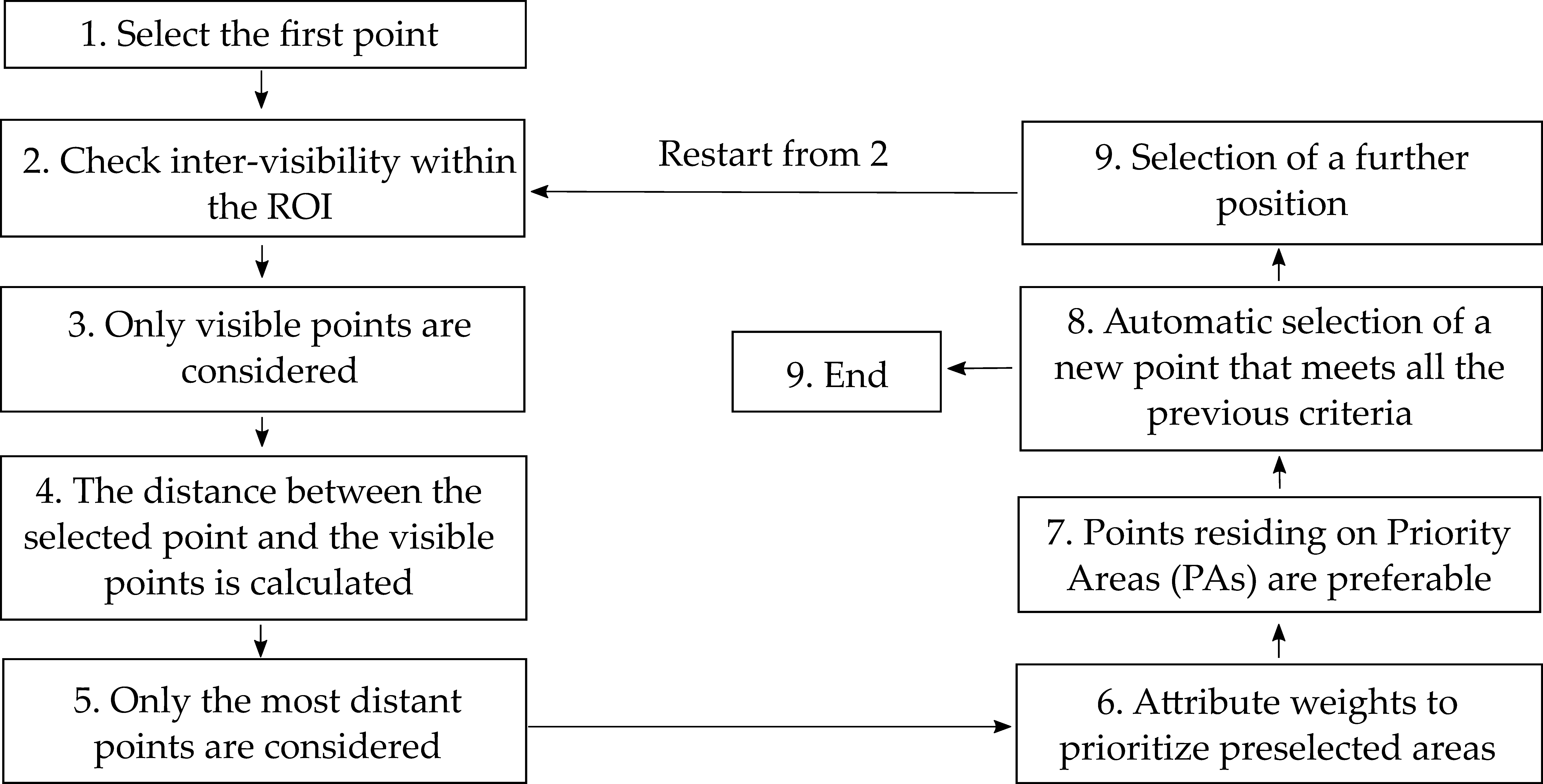
To avoid the involvement of useless data and the consequent increase of elaboration time, the algorithm automatically calculates a region of interest (ROI) for each node. Only points residing inside this region are then considered for subsequent elaborations. The ROI extension depends on the landslide geometry and on the monitoring system used, but it generally coincides with the maximum distance at which two sensors can communicate properly (D_max). Given C, the point of view of X, Y, and Z coordinates, the region is defined by a cube whose farthest points are (X − D_max; X + D_max; Y + D_max; Y − D_max; Z + D_max; Z − D_max). The best positions are thus selected automatically, except for the first one, which is chosen in a semiautomatic way. The user manually selects by clicking on the point cloud with pointer P₁. The algorithm automatically calculates a second ROI (hence ROI_P1), smaller than the previous one, inside which the first point is chosen. The choice is made by means of an iterative procedure, during which n P₁ within ROI_P1 (i.e., the region of interest around P₁) are selected randomly. For each of them, visibility analysis is computed. As a result, the point from which more points are visible is selected as the first point. This helps in positioning P₁ close to the desired area while having a high visibility. The choice of P₁ with low visibility could indeed compromise the results.

2.1. Visibility Analysis

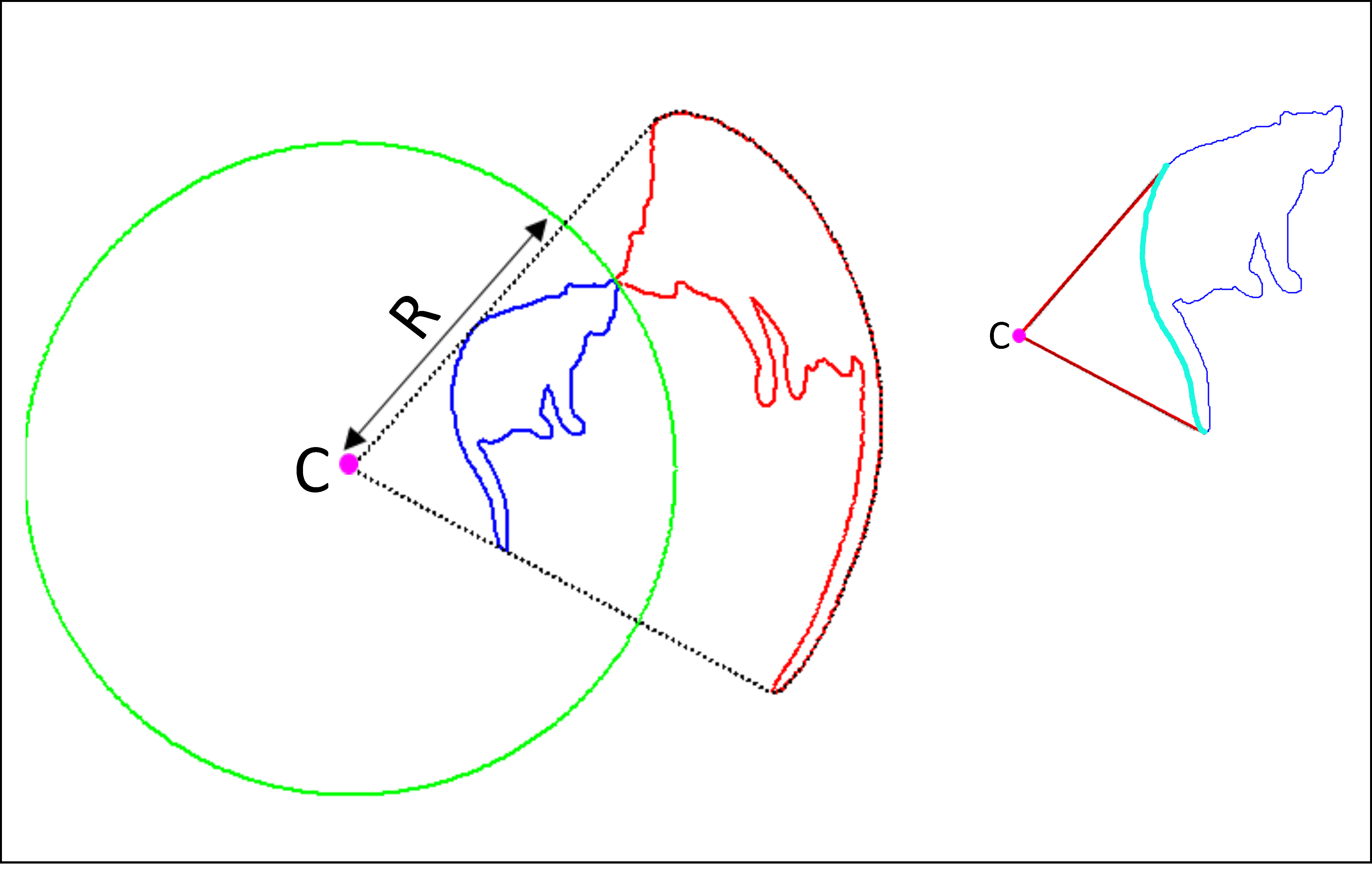
To face the problem of inter-visibility between nodes, the Hidden Point Removal operator proposed by Katz et al. (2007) was applied. The operator is a simple algorithm to determine visibility in point clouds without performing surface reconstruction. It first transforms the points of the cloud by means of spherical flipping inversion, and then computes the convex hull of the set containing the viewpoint and the transformed points [35]. A point is then marked visible from a given point of view if its inverted point lies on the convex hull (Figure 3) [33]. The operator is easy and fast, and it gives back points that are actually visible. Straightforward solutions are in fact bound to fail, and calculating the LOS between two point is not helpful since, except for extreme cases, a point is always visible, even with high-resolution point clouds. The method has found numerous applications in several domains, is supported by theoretical guarantees, and was explained in depth by Katz et al. [33,34,35,36].

R, the radius of the sphere for spherical flipping, is the only parameter to set. As it increases, more points pass the threshold of the convex hull and are hence market visible [33]. Consequently, a large radius is recommended for dense point clouds and the other way around. It is evaluated by an iterative procedure that considers two points of view at opposite sides, with respect to the object center. R is then defined as the value that maximizes the total number of disjoint visible points [35].

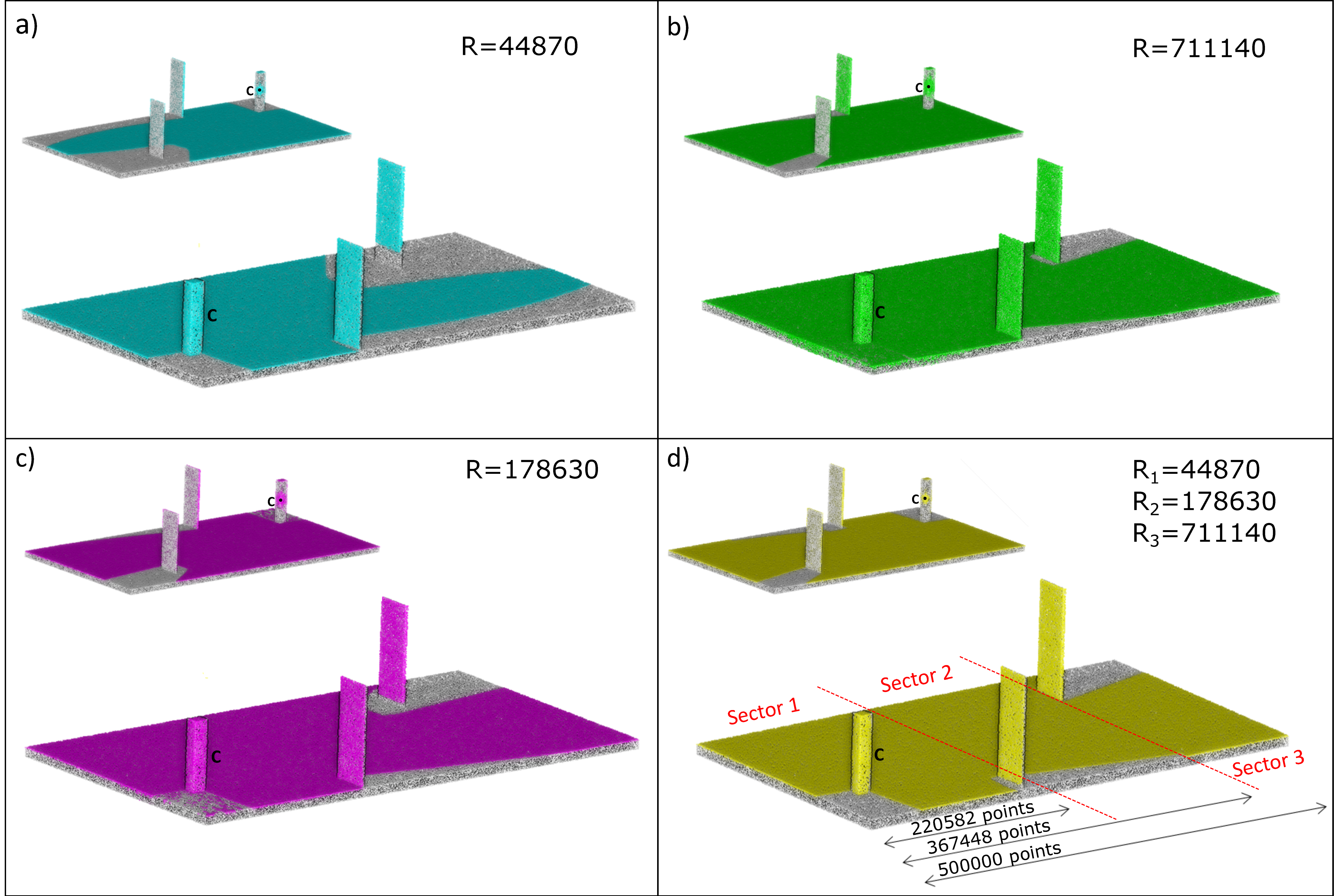
The Hidden Point Removal operator was developed for little objects like small sculptures. In the proposed method, dealing with huge point clouds, R is not constant but changes by increasing the distance from C (point of view) to the target, and it is not only a function of point density (homogeneous in ideal cases). Indeed, it also depends on the amount of points residing within a cuboid centered on C and having a half diagonal (D/2) equal to the distance from C to target. As shown in Figure 4d, given a point cloud (P), the number of involved points obviously grows with distance. The higher D/2 is, the higher the number of points is. In this sense, to correctly apply the operator, the distance has the same role as density: For points closer to C, a small R is recommended, while for farther points, a larger R is more suitable, as demonstrated in Figure 4, where the same R is not optimal for both closer and the farthest points. Too-high R values produce false positives (i.e., nonvisible points marked visible, Figure 4b), and too-low values originate false negatives (i.e., visible points marked as nonvisible, Figure 4a). Choosing a medium value for R is not a good solution since it involves a high number of false positives for short distances and false negatives for longer distances. To solve this problem, the point cloud was split in s cubic sectors centered in C, and R was evaluated for each of them. As a result, optimal R increases by moving away from C (Figure 4d). If the point cloud is divided in s sectors, visibility analysis is computed s time. For each of them, all points between C and sector s (included) were considered, but only the ones that are within sector s are marked as visible or nonvisible. Obviously, the more the sectors in which P is split there are, the more accurate the visibility-analysis results are and the higher the running time is.

To reach the goal of the present work, the Hidden Point Removal operator was applied to a landslide 3D point cloud. Since monitoring sensors (regardless of the type) generally lies on the ground, it is necessary to split the original point cloud in terrain and vegetation point clouds, to avoid the placing of sensors on points representing vegetation. Indeed, in the landscape field, a major obstacle in terms of visibility is vegetation, and monitoring devices are usually installed on the terrain. Therefore, the operator is applied to the whole point cloud, but only terrain points are considered as points where the network could be installed. For distance calculation and computation concerning preselected areas, the point cloud terrain is also the required datum. Vegetation is only involved in visibility analysis. As a result, providing as inputs the point cloud vegetation (PCV), the point cloud terrain (PCT), and the point-of-view coordinates (C), the algorithm returns visible PCT points from C. Furthermore, in some cases, sensors are not directly touching the ground, but they are fixed on supports (e.g., poles and tripods). The proposed algorithm gives the possibility to consider the height of the support, placing points where sensors would effectively be placed; that is fundamental for visibility analysis.

Given h, the support’s height, visibility analysis was computed once h was added to the P_i Z component. If installation on n nodes was required, the Hidden Point Removal operator was applied for each of them for all sectors. Since complete network inter-visibility is required, one can note that node locations are selected between points that are visible from P₁ to P_(i-1), e.g., the choice of P₄ is between points that are visible from P₁, P₂, and P₃.

It is worth noting that obtained visible points lie on the ground, while, in the field, sensors must be in LOS with other sensors, raised in the turn of h. The assumption was that a point raised by h was visible from a given point of view if the same point lying on the ground was visible. Problems come in harsh situations where there is a lot of dense vegetation, such as tall grass, and a minimal amount of terrain points is visible from C. In this case, the algorithm could underestimate the visible points from C, and it could be necessary to ask the algorithm which terrain points would be visible if they were raised by h. To solve this problem, it should be necessary to raise each PCT point (point cloud terrain), one by one, verifying if they lie on the point cloud convex hull. This means that, if the PCT is made by one million points, for each point of view, the operator should be applied one million times: Each time a different PCT point should be raised by h, visibility should be computed and the same point should be lowered by h. This version could be the best solution in areas with low visibility, as well as in areas with not many suitable points to install a device, but it obviously takes too much elaboration time, especially when dealing with big clouds. For this reason, considering the size of the employed point cloud, the authors decided to test the algorithm rising only P_i by h.

2.2. Distribution

For the geometrical deployment of the sensors, with the aim to have equal distribution in space, the Euclidean distance with already selected ones for each P_i was computed. Only the farthest points were then considered to avoid two or more close monitoring devices or areas with no sensors at all. The procedure was carried out by associating weights to node inter-distances.

Given X_(i-1), Y_(i-1), and Z_(i-1), the coordinates of P_(i-1), and X_i, Y_i, and Z_i, the coordinates of P_i,

$$Distance=\sqrt{{\left(X_{\left(\mathrm{i}-1\right)}-X_i\right)}^2+{\left(Y_{\left(\mathrm{i}-1\right)}-Y_i\right)}^2+{\left(Z_{\left(\mathrm{i}-1\right)}-Z_i\right)}^2}$$

(1)

P_i is selected among the farthest points of the PCT from the already chosen points. The remoteness is evaluated by calculating the product of all the distance obtained with Equation (1), between P₁, …., P_i-1 and all the points of the PCT.

2.3. Priority Areas (PAs)

A step that allows the user to prioritize sensors’ deployment in selected portions of the point cloud was added to the algorithm. It aims to give different levels of relevance to distinct areas of a landslide, avoiding the absence of monitoring devices in significant areas. The boundary of these sections (priority areas, PAs) is made manually by the user, and a file with the XYZ coordinates of points residing inside these areas must be uploaded as an input.

In detail, the m farthest points obtained from the distance evaluation (Equation (1)) are pointed out. If between them there are some points residing in PAs, then P_i is selected among those ones. If there is no intersection between the farthest points of the PCT (point cloud terrain) and PAs, then P_i is the farthest point of the PCT from P₁, …, P_i-1. It goes without saying that the choice of m depends on how important the inter-distance is when prioritizing these areas. This makes sure that the user’s experience and knowledge play an important role in the procedure, despite the automatic nature of the tool. Prioritized areas can be areas closer to element at risk, region that have higher displacement values, the most accessible zones, the most stable points, or any areas where the user would like to place devices.

3. Results

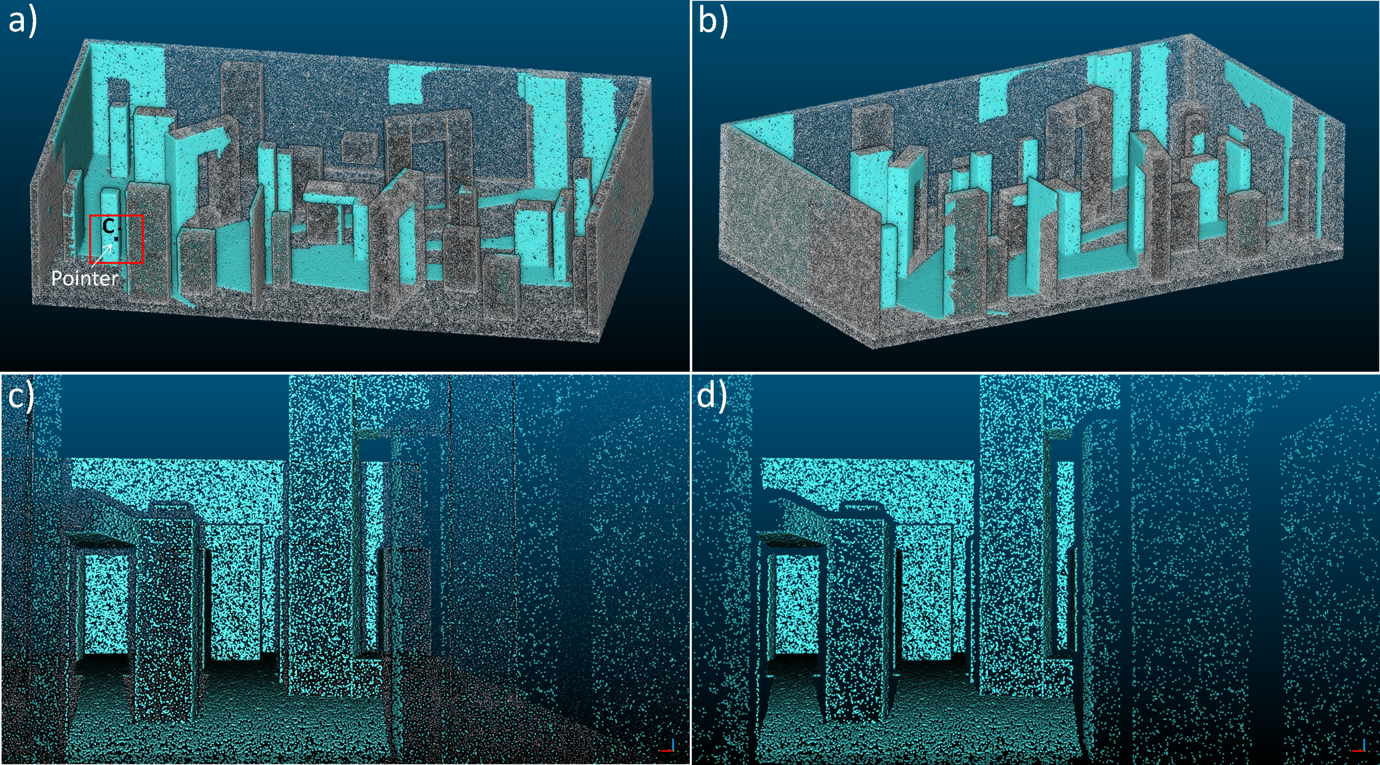
To check the reliability of the proposed algorithm, and with the aim to make the function of the code easy to understand step by step, a 3D model was produced and subsequently transformed into a 3D point cloud. The model was built to have low visibility and to highlight the WiSIO ability in positioning a network, ensuring complete inter-visibility. Furthermore, it allows users to easily perceive visibility from a given point of view (Figure 5). The model was designed on AutoCAD 3D (Autodesk, v. 20.0) and transformed into a 3D point cloud (made by approximately two million points) with CloudCompare (v. 2.10). First, validation was done by selecting generic point of view C, evaluating visible points from C, and exploiting the camera/eye center visualization function of the CloudCompare software (Figure 5). As shown in Figure 5d, all points detected as visible from WiSIO were indeed visible from C (in cyan), since there was no overlap of points. On the other hand, a small number of false negatives were reckoned up due to the precautionary R chosen for the test. The problem of false negatives can easily be solved by increasing the number of sectors. The higher the number of sectors is, the lower the number of false negatives and the higher the running time, as shown in

Table 1. Number of false negatives obtained with various sectors. Test 1 results are shown in Figure 5.

	Radius, R (m)						False Negatives	Running Time
Test 1	Sector 1	Sector 2	Sector 3	Sector 4	Sector 5			(min)
	44,568	354,019	1,119,508	1,774,301	4,456,843		10,504	0.350
Test 2	Sector 1	Sector 2	Sector 3	Sector 4				(min)
	44,568	354,019	706,362	2,812,078			25,120	0.317
Test 3	Sector 1	Sector 2	Sector 3	Sector 4	Sector 5	Sector 6		(min)
	44,568	223,371	706,362	2,233,713	4,456,843	5,610,833	4131	0.393

, where data of three different approaches are reported. Note that Test 1 is the approach whose results are shown in Figure 5.

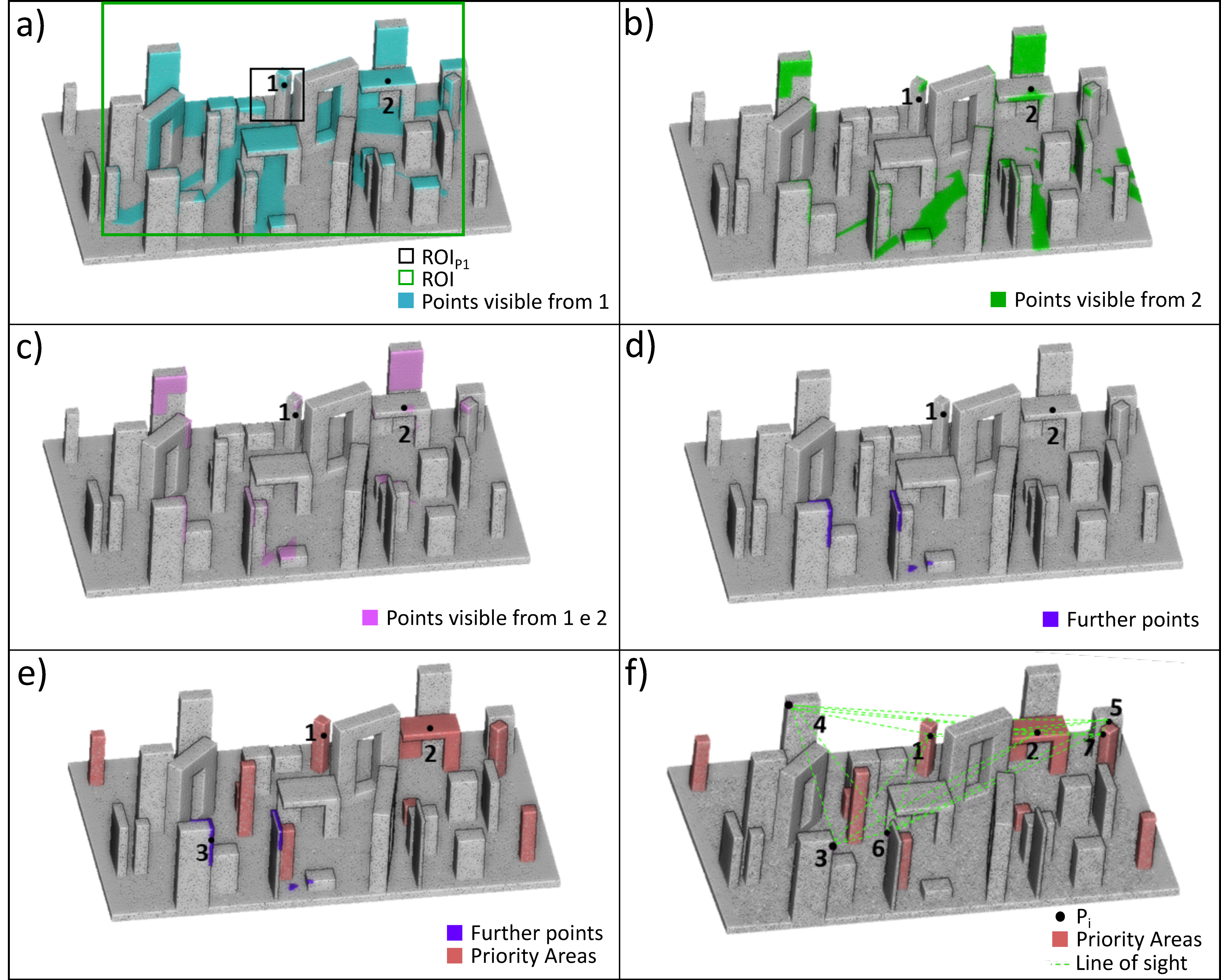
Only one generic point cloud P, made by 1,972,852 points, was used, since no vegetation was present in the model. Figure 6 illustrates the whole elaboration made by WiSIO to point out seven node positions, carried out in 3.33 minutes. Walls were removed to better display all the involved P_i. To detect P₁, the iterative procedure was repeated three times. The automatically evaluated ROI around P₁ (ROI_P1) is depicted as a black box in Figure 6a. Moreover, some objects were randomly selected in the model and uploaded as PAs (in red in Figure 6e,f).

Five sectors were used whose respective radius are those reported in Table 1, Test 1. The test was also repeated, changing the quantity of points to evaluate the amount of time required by varying the size of the point cloud (

Table 2. Different running times for different point numbers.

Point Numbers	Running Time
427,920	0.85 min
1,972,852	3.33 min
2,000,000	3.61 min

). It is worth noting that P₃, P₄, and P₆, were outside priority areas since no farther points overlapped with them (Figure 6e). All selected points were in LOS with respect to the others and equally distributed in space, and four of them resided in areas marked as Pas, despite the designed harsh environment (Figure 6f).

Field Application

The method was applied in the field for the installation of the Wi-GIM system, a Wireless Sensor Network measuring node inter-distance by means of ultrawide-band technology. For more details about the system, please refer to Mucchi et al. [18] and Intrieri et al. [28]. The devices worked properly in LOS conditions; thus, aimed deployment of the sensors could widely improve their efficiency. For better evaluation of the improvement, Wi-GIM was installed in the Roncovetro landslide, as previously done by Intrieri et al. [28]. During this first monitoring period, system accuracy and precision were analyzed. 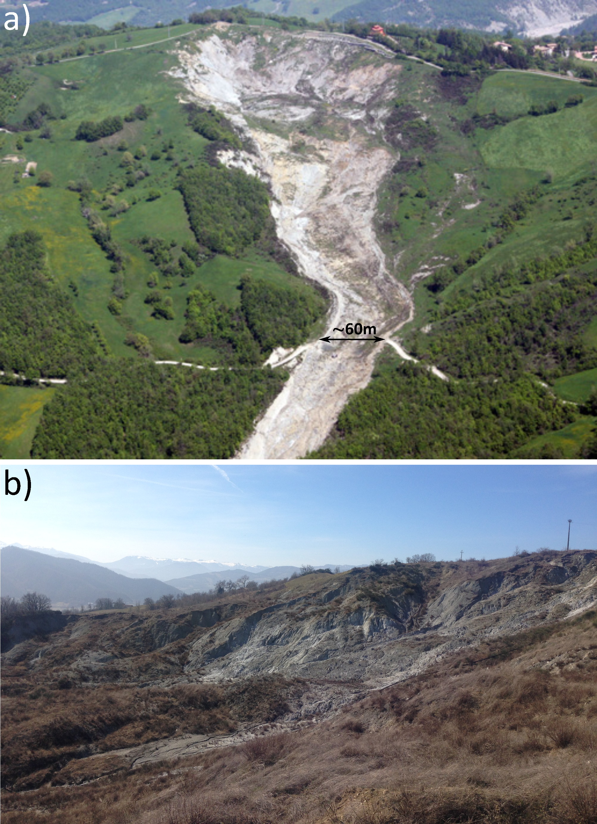While precision ranged from 2 to 5 cm, the medium recorded error of the distance was about 75 cm, and it was strictly connected to both the presence of obstacles and the low-cost nature of the system [28]. However, this large error did not compromise the effectiveness of the system since it focused on relative distances and not absolute ones. The slide is a 2 km long mudflow located in the Emilia Romagna Region, Central Italy (Figure 7). The site was particularly suitable for the application of WiSIO due to its dimensions, the amount of vegetation, and the presence of geomorphological highs and lows that make it harsh even in terms of visibility.

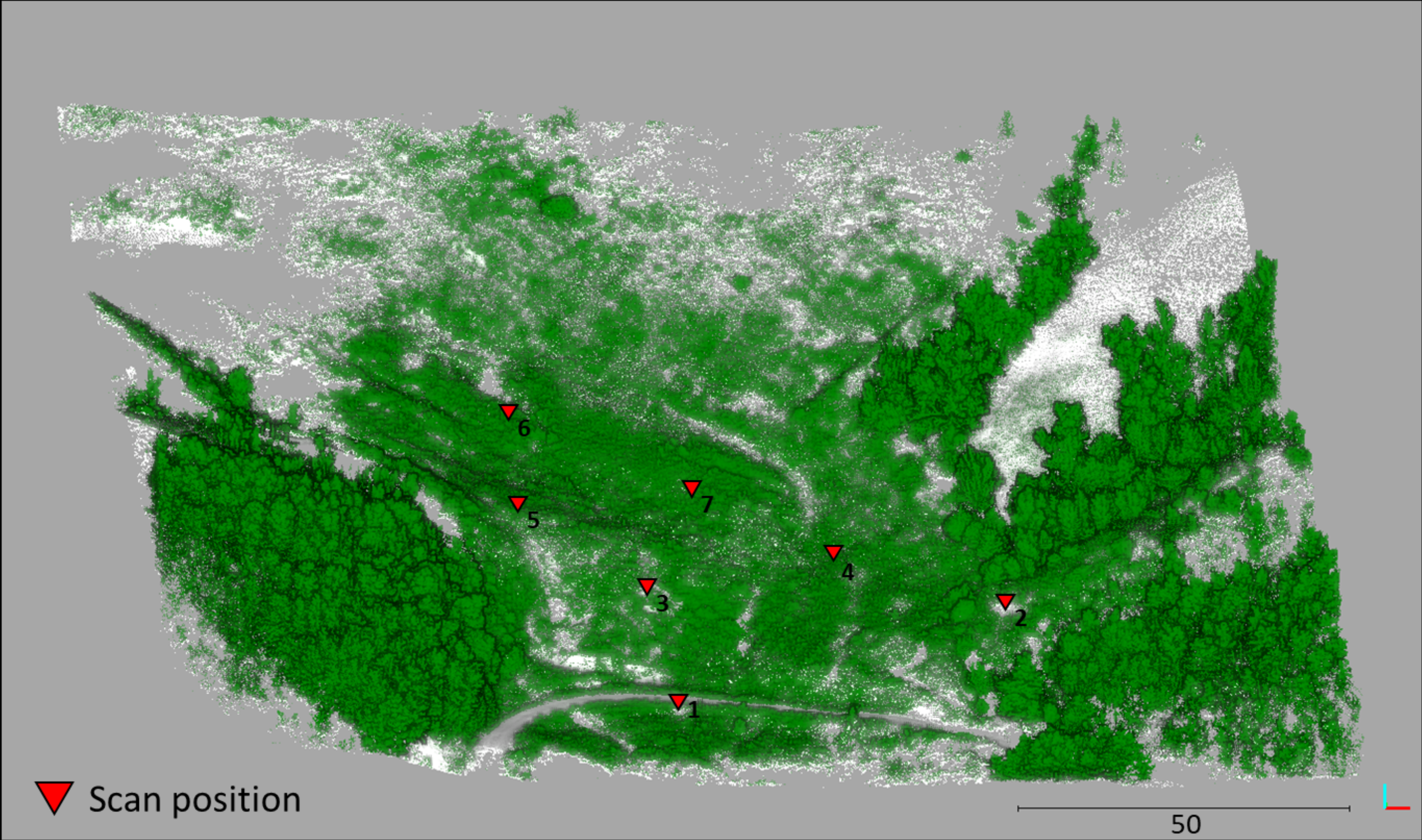
The 3D point cloud was obtained with a terrestrial laser-scanning survey in which seven different scans were acquired from different positions in order to limit the shadow areas (Figure 8).

After being aligned, a vegetation filter was applied to split the point cloud into a PCV and a PCT. As in 2016, sensors were installed on 1.5 m high iron poles, as consequently considered in the parameter settings. The ROI was fixed at 100 m, i.e., the maximum distance at which Wi-GIM sensors properly communicate [28].

Due to the low visibility of the site, the authors wanted to exclude the positioning of one or more sensors in areas with scarce visibility, since it would have compromised the best positioning of the subsequent sensors. WiSIO places devices in LOS to each other but without considering if the surrounding areas are highly visible. In stress conditions like the Roncovetro landslide, due to the presence of vegetation, as well as terrain roughness and slopes, it may happen that a sensor is correctly positioned in LOS with the others and is following the distance criteria, but in an area from which few points are visible, sacrificing the positioning of succeeding devices. To prevent this, the geomorphologically highest locations were selected as PAs. To automatically select these areas, simple computation was performed. Cells were extracted by moving a sampling cube of fixed dimension (5 m in the presented work) on the point cloud terrain. For each of them, the medium elevation value (Z_med) and the medium of the 10 highest elevation values (Z_max) were calculated. PAs were thus defined as points residing in cells whose Z_max–Z_med passed the threshold of 2 m (Figure 9). Note that the choice of calculating Z_med as mentioned above, instead of directly using the maximal-elevation value of each cell, was done to avoid outlier issues. All input parameters used for the Roncovetro application are listed in

Table 3. Summary of input parameters used for Roncovetro application.

h 1	ROI	ROIP1	m2	P1 Iterations
1.5 m	100 m	5 m	20%	5
R Sector 1	R Sector 2	R Sector 3	R Sector 4	R Sector 5
3593 m	18,010 m	71,700 m	180,104 m	285,446 m

Note: ¹ Iron-pole height. ² Value expressed as percentage of points visible from Pi.

.

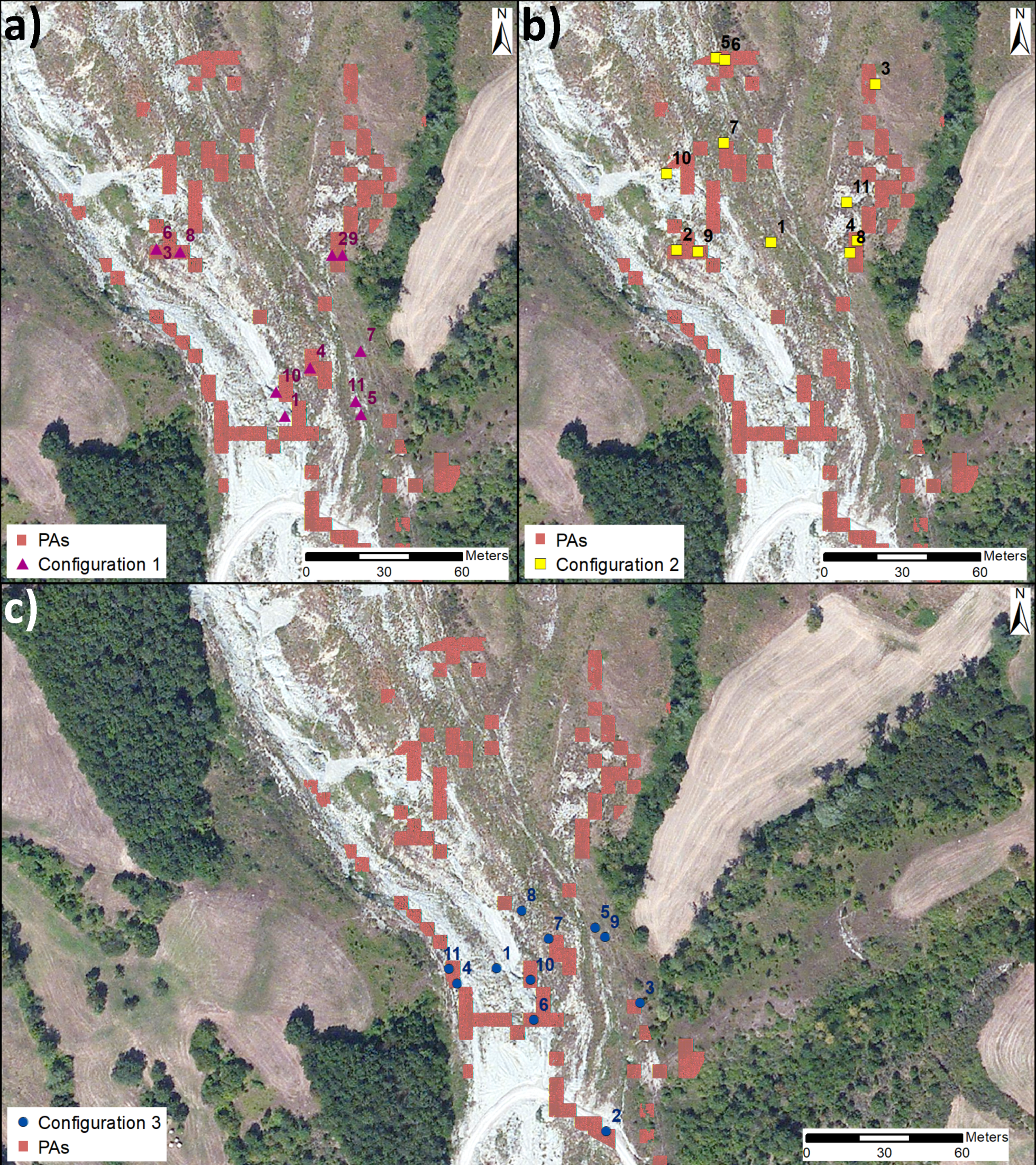
The selection of P₁ strongly influenced the whole deployment. As an example, Figure 9 shows three different configurations obtained by changing original position ROI_P1, which framed an area of 5 m around P₁. In Cases 1 and 3, it was situated in central and easy-to-reach positions, while in Case 2, C was situated a bit farther upstream. The most satisfying configurations were the ones in Cases 2 and 3, due to their distribution in the landslide’s body and to the presence of one or more stable points located outside the landslide. Since it was the intention of the authors to install the system in the same area where it was in 2016 (see Figure 10c,d), aiming at a complete comparison of the collected data, the new installation of the Wi-GIM system was done in February 2019, following Configuration 3 (Figure 9c).

4. Discussion

As shown in Figure 9c, seven out of eleven devices lay in PAs. A non-PA point was, however, P₁, whose position was manually picked out. The remaining three were outside them, as a result of the relationship between distance and m value (set equal to 20% of points visible from P_i). All sensors were effectively in LOS, as demonstrated by the analysis carried out with the camera/eye center-visualization function in CloudCompare. Despite this, the acquired data showed a lack of three couples, i.e., 3–11, 2–7, and 4–5. This leak could be due to changes in vegetation or to problems related to the decawave. Concerning vegetation, please note that, due to logistic problems, three months passed from scan survey to installation. This period may have led to some changes on the field due to animal transitions or branches falling. Furthermore, some problems were already encountered in the past because of the low-cost nature of the decawave [28].

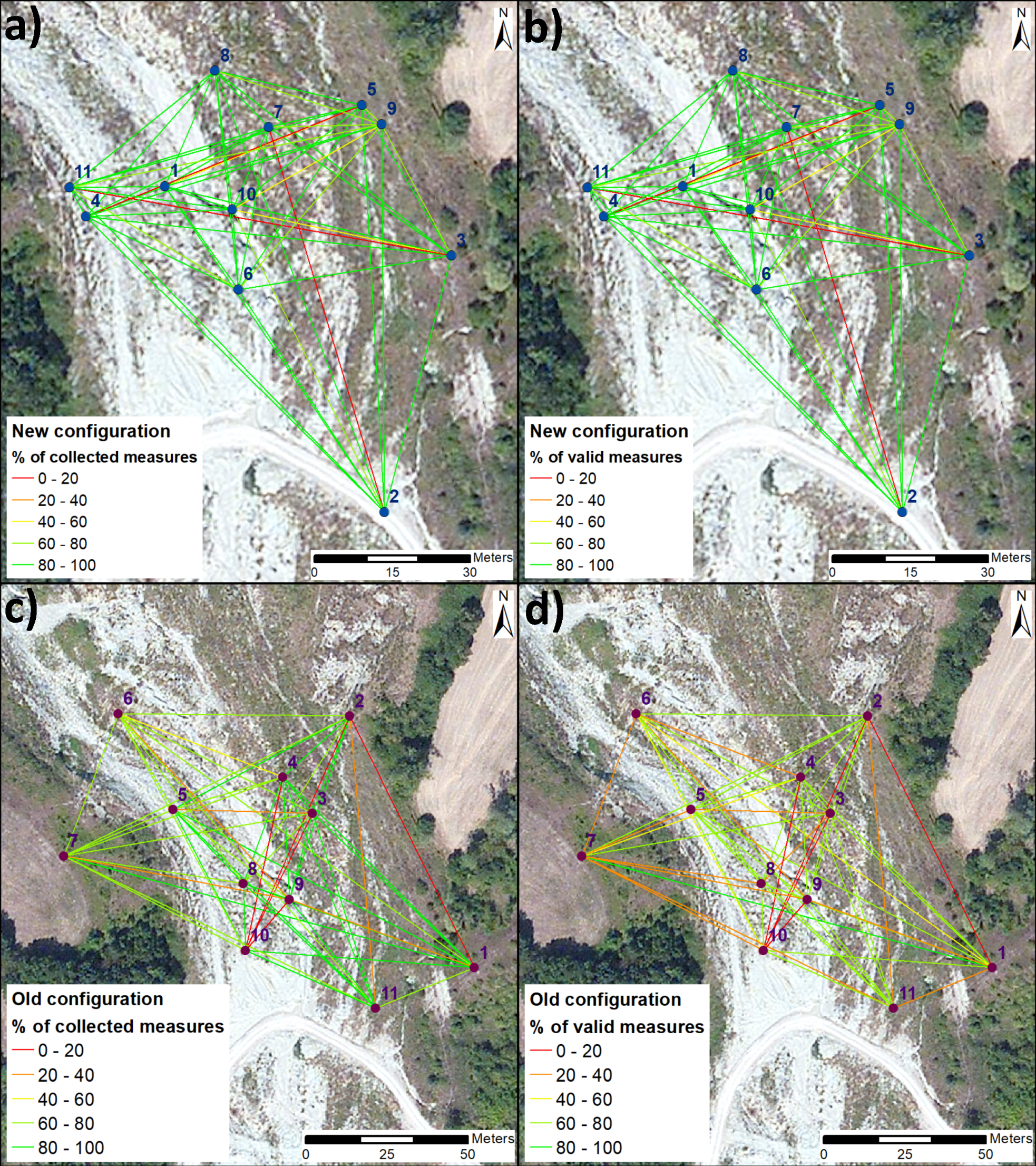
To better understand the effectiveness of WiSIO, a comparison between data from the 2016 installation and actual ones was pointed out, considering the amount of acquired data as their worth. The percentage of collected and valid data in the old, as in the new, configuration is shown in Figure 10, where valid data means the data with no outliers or zero values. In Figure 10a,b, the percentages of collected and valid measures, respectively, are reported in the form of colored links for each couple of nodes. As evident, values were between 90% and 100% for all couples, except for the four abovementioned pairs and for couples 1–5, 3–10, and 9–10. In these three last cases, both collected and valid data were between 45% and 50% (Figure 10a,b). 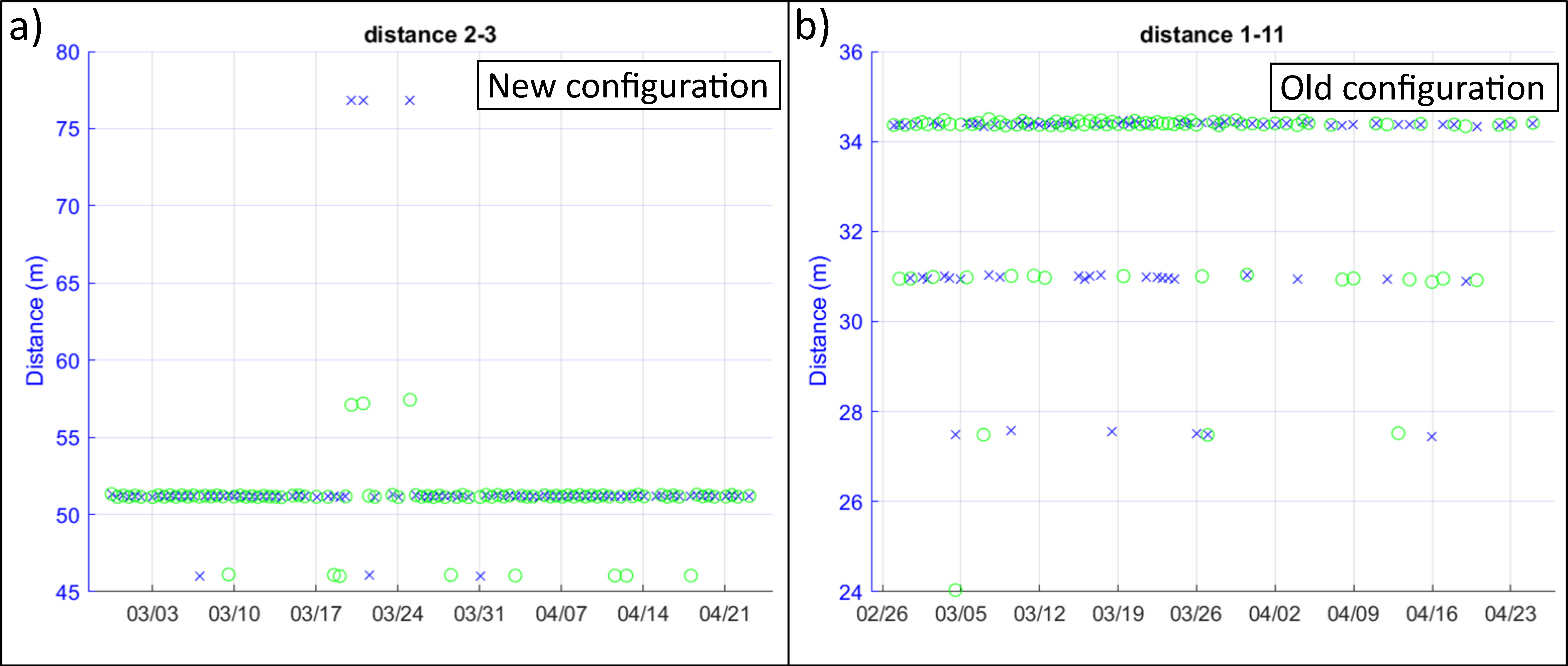The same procedure was done for data obtained with the old configuration, i.e., the 2016 one (Figure 10c,d). In this case, the percentage of collected data was less than 60% for 10 couples, and the percentage of valid measures did not reach 60% for 22 couples. That means that not only were fewer data acquired in the old configuration due to non-LOS problems, but data quality was most importantly worse, as well. Indeed, in the old configuration, data acquisition did not guarantee validity, as it is for the new configuration, where there was no discrepancy between the percentage of collected and valid data. Considering couples whose percentage of valid data was at least 60% as suitable, 50 out of 56 couples were suitable in the new configuration (i.e., 89.3%), instead of 34 out of 56 in the old one (i.e., 60.7%); thanks to WiSIO, the amount of valid data increased by 28.6%. An example showing this improvement is reported in Figure 11. Couples 1–11 from the old configuration and 2–3 from the new one were considered due to similar distance, position, and visibility conditions. They both collected at least 60% of the measures (even though it is strongly visible from Figure 11 that there was loss of data in couple 1–11) but yielded different results in terms of validity. Indeed, couple 1–11 presented several problems with outliers and multipath effects, issues which were eased in couple 2–3 (Figure 11).

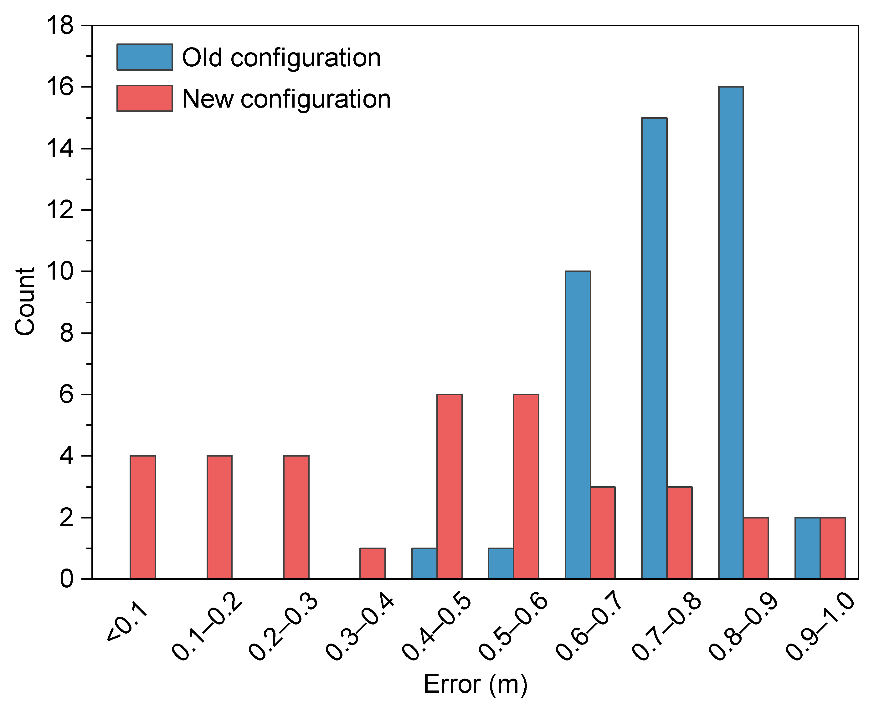
Contrary to precision, whose values remained in the range of 2 to 5 cm once outliers were removed [28], WiSIO also had an effect on data accuracy, affected by the presence of obstacles. Comparing the offset between real distances and Wi-GIM-measured distances, it was clear how the placement of sensors in LOS contributes to increasing accuracy (Figure 12). The histogram shows the offset between real and measured distances (“Error” in the graph) for all node couples in the two configurations. It is clearly visible that, in the old configuration, the error was higher in almost all couples due to the presence of obstacles, whereas it is lower and much more distributed in the new configuration.

5. Conclusions

With the aim of finding the best position to place WSN devices requiring free LOS, a MATLAB tool called WiSIO was developed. The algorithm finds the best device deployment by following three criteria: inter-visibility by means of the Hidden Point Removal modified operator, equal distribution, and positioning in preselected priority areas. This works directly with 3D point clouds without performing any surface reconstructions, leading to skipping the process of generating surface models avoiding errors and approximations.

A 3D model of a harsh environment with low visibility was developed to validate WiSIO. Results highlighted good correspondence with reality, showing just a few false negatives (i.e., visible points marked as nonvisible). Precision could, in any case, be improved by increasing the number of sectors and evaluating the radius for each of them. The sectors there are, the fewer the false negatives or/and false positives, and the higher the running time. In this framework, the automatic configuration of a ROI, allowing to process only points inside it, helps in saving time, avoiding the use of useless data. Its size is a parameter under the control of the user, able to govern the area to place devices without cutting or modifying the original point cloud. Moreover, the choice of m (the number of points to consider checking if some of them lie in PAs) allows the user to evaluate the importance of PAs with respect to the equal distribution of the devices in the field. This, together with the detection of P₁ within ROI_P1 and the selection of PAs, ensures that users apply their knowledge in the procedure, despite the automatic approach of the code.

WiSIO was applied to the real case of the Roncovetro landslide, Central Italy. There, an ultrawide-band WSN, i.e., the Wi-GIM system, was installed, as previously done in 2016. The comparison of data acquired by the system positioned with and without the help of the proposed algorithm allowed for a complete analysis of the efficiency of the method. Both the quality and quantity of the acquired data were analyzed through a comparison with the 2016 data. According to the results, almost all devices were in LOS with each other, evenly distributed in space, and seven of eleven devices lay in Priority Areas. As a matter of fact, 87.5% of measurements were collected by the master node, and, between them, 89.3% were good enough to be considered reliable data with respect to 2016, when the acquired measurements were 82% and only 60.7% were valid. The presented results are very promising, showing how a simple elaboration can be essential to have more and more reliable data.

The continuous growth of new technologies for the development of increasingly high-resolution 3D point clouds (i.e., drone laser scanners and high-resolution cameras) could still improve the reliability of the presented approach that is highly dependent on the data source.