A Multilevel Mapping Strategy to Calculate the Information Content of Remotely Sensed Imagery


1
Department of Geo-Informatics, Central South University, Changsha 410083, China
2
Institute of Surveying and Mapping, Information Engineering University, Zhengzhou 450001, China
*
Author to whom correspondence should be addressed.
ISPRS Int. J. Geo-Inf. 2019, 8(10), 464; https://0-doi-org.brum.beds.ac.uk/10.3390/ijgi8100464
Submission received: 11 September 2019
/
Revised: 8 October 2019
/
Accepted: 20 October 2019
/
Published: 22 October 2019
(This article belongs to the Special Issue Uncertainty Modeling in Spatial Data Analysis)
Abstract
:Considering the multiscale characteristics of the human visual system and any natural scene, the spatial autocorrelation of remotely sensed imagery, and the multilevel spatial structure of ground targets in remote sensing images, an information-measurement approach based on a single-level geometrical mapping model can only reflect partial feature information at a single level (e.g., global statistical information and local spatial distribution information). The single mapping model cannot validly characterize the information of the multilevel and multiscale features of the spatial structures inherent in remotely sensed images. Additionally, the validity, practicability, and application range of the results of single-level mapping models are greatly limited in practical applications. In this paper, we present the multilevel geometrical mapping entropy (MGME) model to evaluate the information content of related attribute characteristics contained in remotely sensed images. Subsequently, experimental images with different types of objects, including reservoir area, farmland, water area (i.e., water and trees), and mountain area, were used to validate the performance of the proposed method. Experimental results show that the proposed method can not only reflect the difference in the information of images in terms of spectrum features, spatial structural features, and visual perception but also eliminates the inadequacy of a single-level mapping model. That is, the multilevel mapping strategy is feasible and valid. Additionally, the vector set of the MGME method and its standard deviation (Std) value can be used to further explore and study the spatial dependence of ground scenes and the difference in the spatial structural characteristics of different objects.
1. Introduction
With the remarkable development of earth observation systems and technology over the past decades, the acquisition technology of remote sensing imagery shows some new development trends including multiplatform, multisensor, and multiangle approaches [1,2,3]. Meanwhile, the remote sensing images obtained also possess a number of key features such as very large volumes, diverse varieties, and fine-grained resolution [4,5]. High-resolution images become a more important data source in image processing and applications, e.g., classification, change detection, and image segmentation, especially as the resolution of images becomes increasingly higher [6,7,8,9].
In the meantime, compared with the low- and middle-resolution remote sensing images, high-resolution images can provide more detailed feature information of ground objects, such as texture size, geometric structure, and spatial layout [10]. Therefore, spatial structural features have become one of the most remarkable features of high-resolution images. Additionally, the structural characteristics of high-resolution images are more stable in comparison with spectrum features and are also able to reflect the spatial relationship between the internal organization characteristics of the object and its external environment [11,12]. Moreover, different types of objects contained in high-resolution images exhibit different degrees of structural characteristics. This is the reason why the spatial structure of high-resolution images has multiscale and multilevel characteristics [13].
Therefore, during image processing, the question of how to reasonably and effectively describe and evaluate the amount of information from attribute features (e.g., spectral features, spatial structural features, etc.) in remote sensing images (especially for high-resolution images) has become one of the key issues in improving the utilization ratio of remotely sensed data [14,15,16]. Meanwhile, the measurement results from imagery can be applied to subsequent image processing, such as image interpretation and information extraction. Additionally, they can be used as criteria for data screening to reduce the blindness of data selection and lower the cost of data [17,18,19].
Although in information theory information entropy is commonly regarded as a valid indicator for estimating the information uncertainty of images [20,21,22], the traditional Shannon entropy of images considers only related information from global probability statistics in images but neglects local feature information (e.g., spatial distribution, organization structure) and other useful information such as visual perception [23]. That is, the classic image entropy merely describes partial planar information contained in images from a quantitative perspective and cannot reflect more important and critical feature information contained in images at a deeper level [24]. Furthermore, in the case of different imaging patterns or different imaging conditions, the gray properties of different source images of the same ground scene have considerable differences at various times. This phenomenon could imply that the measurement result of a single source image cannot accurately and validly reflect related attribute feature information contained in a ground scene.
Notably, some of the traditional image entropy models based on information theory and the corresponding improved methods mainly explore and study the influence of related factors on the amount of information contained in images, such as the grayscale quantitative level, noise, spatial resolution, and correlation within or between bands [25,26,27]; for example, various models focus on the relationship between information content and the signal-to- noise ratio (SNR) [28], the effect of resolution (e.g., spatial resolution, radiometric resolution) on the information-content characterization of images [29,30,31,32,33], and a number of the Markov model-based information measurement methods for describing spatial correlation. Moreover, some scholars construct the measurement model used in characterizing spatial structures from a new perspective, such as Gao et al., who proposed configurational entropy (also called Boltzmann entropy) to represent related information on spatial structure in geoscientific data [34,35,36]. In addition to all of these methods, our previous work illustrates that the single-level-geometrical-mapping-model-based information measurement approach as a unified metric model can accurately characterize the information from images of global statistical features, local spatial features, and visual perception and is able to distinguish the effects of the different imaging conditions (e.g., light condition, clouds) on the quality and information content of images.
It should be noted that despite the improved performance of these previously mentioned approaches in comparison with traditional image entropy models, some issues still exist, such as parameter settings being difficult to determine, model construction being relatively complicated, and the operational performance of models needing to be further improved [37,38]. Additionally, these measurement models basically do not directly or validly reflect the information of the multilevel and multiscale features of spatial structure inherent in remotely sensed images, which greatly limits the accuracy, practicability, and application range of these methods in practical applications [10].
To better evaluate the information content of related attribute features contained in remote-sensing images, the multiscale and multilevel characteristics of spatial structures are considered [13,39]. In this study, a multilevel-mapping-model-based measurement method is proposed by incorporating a multilevel mapping strategy and the corresponding standard deviation into the modeling process used in information measurement. The present study is a further extension for our previous work.
The remainder of this work is structured in four sections. Section 2 reviews the spatial structure and spatial dependence of images and traditional image entropy. Section 3 presents the multilevel-mapping-model-based computation strategy for evaluating the information content of images. In Section 4, we validate the feasibility and effectiveness of the proposed method through different object types in experimental images and provide a discussion and analysis of the work. Section 5 provides conclusions and has a further outlook for future work.
2. Related Basic Theory
This section will briefly outline spatial dependence and spatial structural features in images and the traditional image entropy model. The detailed descriptions are as follows.
2.1. Spatial Dependence of Images
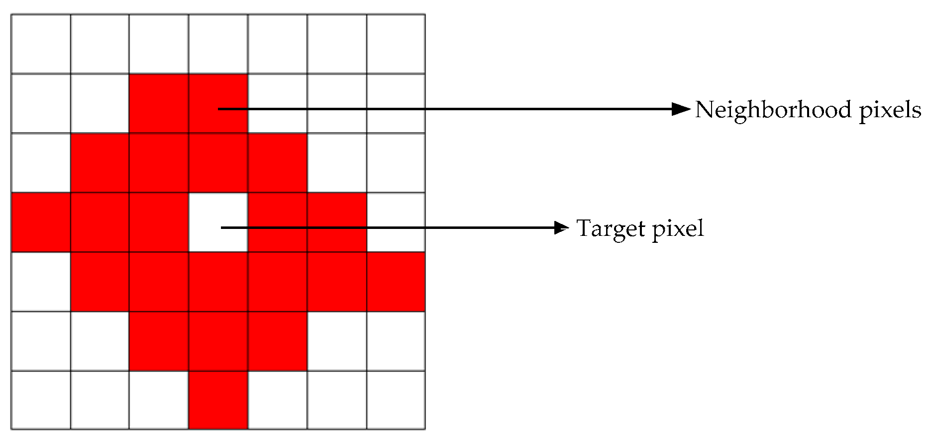
According to the First Law of Geography, everything is related to everything else, but near things are more related than distant things [40], i.e., there is connectivity and correlation between spatial units. Likewise, the attribute information of a single pixel in images has a certain degree of similarity with the attribute information of its neighboring pixels, i.e., the pixels in images are not isolated. That is, remotely sensed images also have a high degree of spatial dependence (i.e., spatial autocorrelation) [41,42]. Additionally, the similarity and correlation of different pixels and corresponding neighboring pixels are usually also different, which directly leads to the regional randomness and internal spatial structural characteristics in images [12]. The description of pixel neighborhood is shown in Figure 1.
Furthermore, compared with the larger difference between the description information of the medium- to low-resolution images in a large-scale ground scene and the small-scale layout structure needing special consideration in the natural scene, high-resolution images contain more feature information, such as texture size, geometric structure, and spatial layout, in which the layout structure of small-scale objects can better depict spatial dependence. With an incremental increase in the resolution of images, the difference in the natural scene and the remotely sensed scene is gradually narrowed [13]. It also indicates, from another perspective, that the introduction of theoretical methods in the field of machine vision into image processing and applications has a certain degree of feasibility [43,44].
2.2. Spatial Structural Characteristics of Images
Remote sensing images are the comprehensive descriptions of object features of a ground scene, which contain not only spectral feature information but also rich spatial information such as texture size, geometrical structure, and spatial layout relationships [45]. In particular, different object types in high-resolution images distinctly exhibit different degrees of structural characteristics, i.e., multilevel characteristics of spatial structures [13]. Thus, high-resolution images can provide additional useful information through spatial structural features for some operations in image processing (e.g., image interpretation and information extraction) [11,46].
The related unified definition or description of spatial structural features of images is proposed in [12]. It is defined as follows.
Definition 1.
The spatial structural feature of images indicates spatial distribution patterns formed in terms of different distributions, different permutations, or layouts of the elements in digital images.
The element here is the basic unit of structural analysis. That is, the pixels of images within different neighborhoods form the regional objects of images with different levels of structure by using different arrangements or distributions. Meanwhile, the multiscale characteristics of pixels lead to the multiscale characteristics of the image structure, which is also closely related to the cognitive scale of the human visual system and the spatial resolution of images [12,13]. In addition, spatial structural features can also compensate to a certain extent for the inadequacy existing between spectral features, i.e., it can reflect more detailed local feature information of ground objects. Essentially, spatial structural features can be described by the distribution of neighborhood pixels or dependencies between pixels in images (see Figure 2) [45].
2.3. Image Entropy
Generally, for a discrete random variable with limited elements, the corresponding probabilities of different elements in are, respectively, . The Shannon entropy of can be computed as follows [47,48,49].
where is the number of elements in the random variable . Statistically speaking, can reflect how much uncertain information the random variable has on average, e.g., if the values of are certain, i.e., = 1, then = 0; when the elements of random variable have equal probability, the value of is maximized. Additionally, the value of varies with the number of elements in the random variable , and its range of values is .
In the field of remote sensing, traditional image entropy is also regarded as one valid quantitative indicator used to evaluate the information content of images. Similarly, a digital remote sensing image is comprised of a finite number of discrete pixels, in which each pixel corresponds to certain grayscale level . Commonly, the pixels of different grayscale levels are randomly filled into different spatial regions. This distribution usually causes different images to exhibit different information [20,33,50]. The formulas for image entropy are as follows.
where is the number of pixels with a certain grayscale level , is the total number of all pixels in the image, and is the probability of different gray levels . In general, the range of grayscale levels in a grayscale image is , i.e., the range of values in image entropy is . The image entropy value, so to speak, is directly related to the degree of change in grayscale levels, i.e., fewer grayscale levels and a more concentrated the grayscale distribution are associated with less uncertain information in images; conversely, more grayscale levels are related to more uncertain information in images. That is, image entropy can reflect the degree of dispersion and uniformity of brightness values of images.
To characterize much more attribute feature information contained in the image, on the basis of introducing the neighborhood information, a multilevel-mapping-strategy-based information measurement scheme is developed by incorporating the mapping idea of the multilevel pixel neighborhood into the modeling process. This method can not only reflect the difference in the information of images on spectrum features, spatial structural features, and visual perception but also eliminates the inadequacy of a single-level mapping model.
3. A Multilevel Mapping Strategy-Based Information Measurement Scheme
3.1. Multilevel Pixel Neighborhood Model
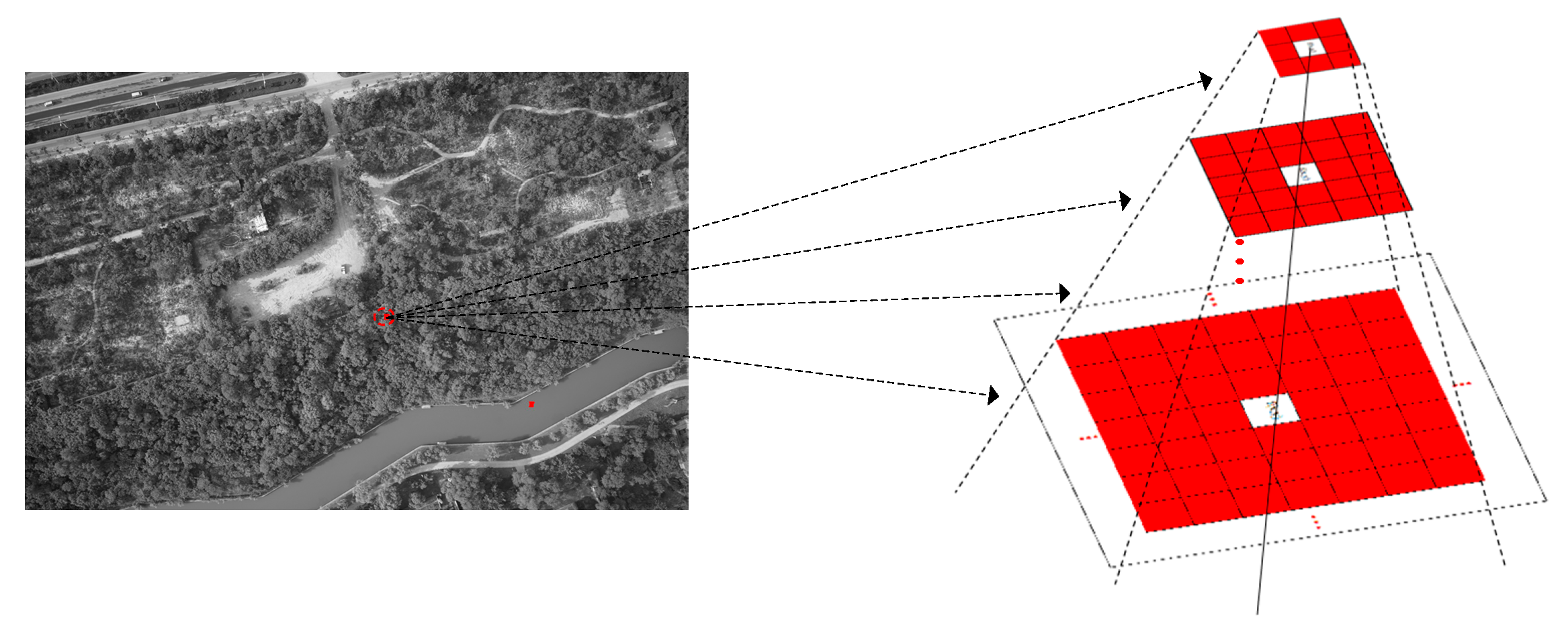
It is noticeable that a spatial structural feature can be reflected by attribute information of the pixel neighborhood or dependencies/correlation between pixels. That is, in essence, the spatial structural pattern of a pixel neighborhood can be used to characterize the spatial structural feature of a single pixel [13]. Furthermore, different ground object types mapped by high-resolution images usually exhibit different degrees of structural characteristics, which leads to the multiscale and multilevel characteristics of spatial structures. Consequently, we attempt here to utilize different levels of pixel neighborhood information to characterize the spatial structural features contained in images (see Figure 3) [45,51,52,53,54,55].
3.2. A Multilevel Geometrical Mapping Entropy (MGME) Model
3.2.1. A Multilevel-Mapping-Strategy-Based Measurement Scheme
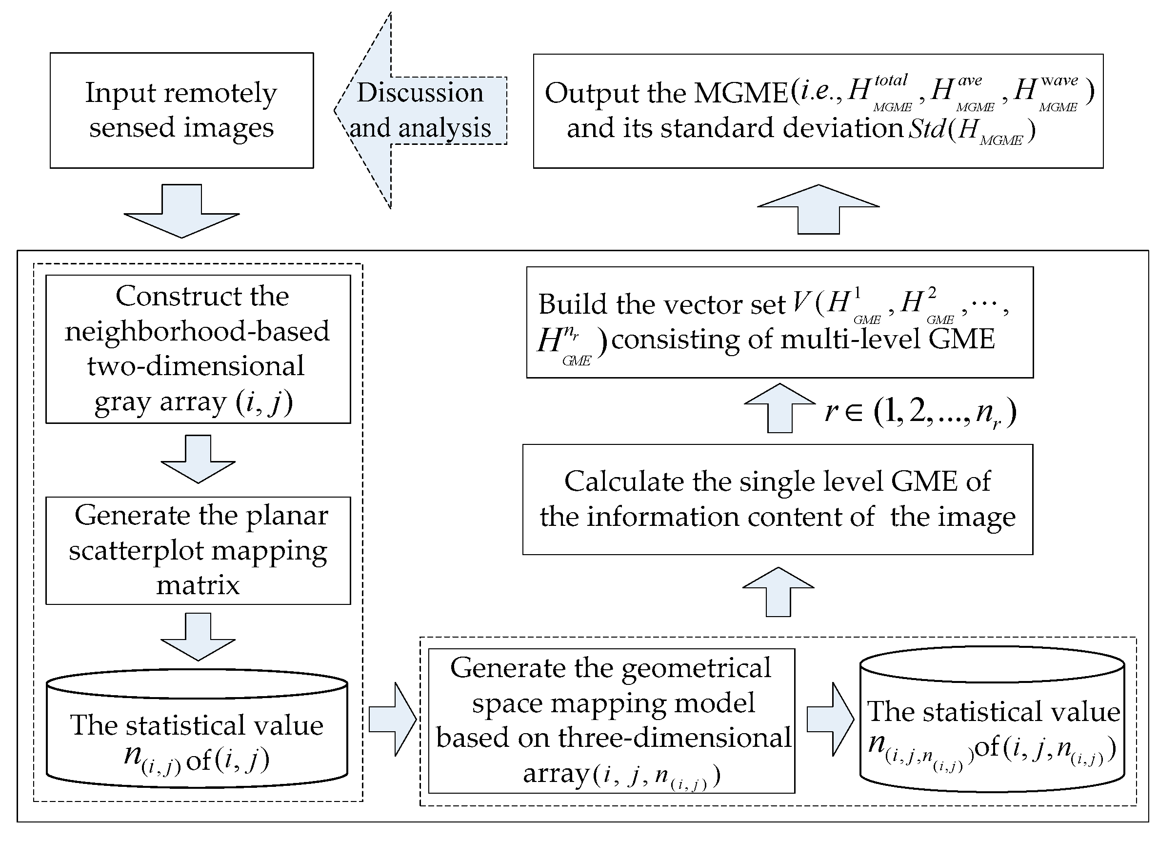
Furthermore, remotely sensed data are the objective descriptions of the object features of a ground scene. These data contain not only substantial spectral feature information but also abundant spatial structural information. To more effectively, reasonably, and accurately characterize and evaluate the information of attribute features contained in images [34,45,56,57,58,59], we present a multilevel mapping strategy to calculate the information content of remotely sensed images, i.e., a multilevel geometrical mapping entropy (MGME) model. The general framework of this approach is described in Figure 4.
3.2.2. Description of the MGME Model
The detailed steps of the MGME model are described in the following text.
First, let us construct a two-dimensional grayscale array using each grayscale value of each pixel and its grayscale mean value within a certain effective neighborhood to validly characterize the information of local spatial structural features near the target pixels in images. The formula is shown in Equation (4).
where is the grayscale value of the s-th neighborhood pixel of the target pixel with grayscale value . When the neighborhood radius of the target pixel is equal to , is the true number of pixels in the effective neighborhood of the target pixel, and the average value is calculated by the ratio of the sum of the practical neighboring pixels of the target pixel to . Additionally, the grayscale array is mapped into the planar mapping matrix by the two-dimensional scatterplot model, and is the statistical value of in the planar mapping matrix.
Second, the three-dimensional array is comprised of the grayscale value of the pixel, the average grayscale value of its neighboring pixels, and the statistical value of the grayscale array . The can be mapped into the geometrical mapping space by the three-dimensional scatterplot model, and is the statistical value of the three-dimensional array in the geometrical mapping space. Thus, the single-level geometrical mapping entropy (GME) is developed by incorporating the mapping ideas of the scatterplot matrices and the statistical values of into the modeling processing. The probability of in geometrical mapping space can be calculated by:
where is the statistical value of , and is the total number of with different values.
Definition 2.
The geometrical mapping entropy (GME) of the image with the mapping probability is defined as:
Third, we further construct multilevel geometrical mapping entropy through combination with a different-level mapping model. The related formulas can be expressed as:
where and are the radius of a different neighborhood window and the maximum neighborhood window, respectively; is the vector set consisting of multilevel GME values; and are, separately, the sum and the average of measurement results of the multilevel-strategy-based measure model; is the weight of the different GME values in the vector set; and is the corresponding weighted average of the multilevel GME.
Last, we validate the feasibility and effectiveness of the MGME model through the experimental results below. Furthermore, we attempt to discuss and analyze the spatial structural features of images using and its standard deviation ().
4. Experiments and Analysis
In this section, a set of experimental data used to validate the feasibility and effectiveness of the MGME model includes the following experimental images.
- A 0.5 m resolution image of a reservoir area located in the Zhengzhou region, obtained from the DigitalGlobe platform in 2018;
- An image of farmland obtained from the UC Merced Land Use Dataset with USGS National Map Urban Area Imagery in 2010 with 0.3 m resolution [60];
- A UAV image of a local area in the district of the lower and middle reaches of the Yellow River in 2015;
- Landsat TM image of a mountainous region provided by NASA.
4.1. Experiment 1
In this experiment, we used this group of experimental data to verify the performance of the MGME model (Figure 5a–d) and further deeply analyze and discuss the qualitative and quantitative results. The max radius of the multilevel mapping model we adopted is mainly in reference to empirical values employed in these projects [61,62].
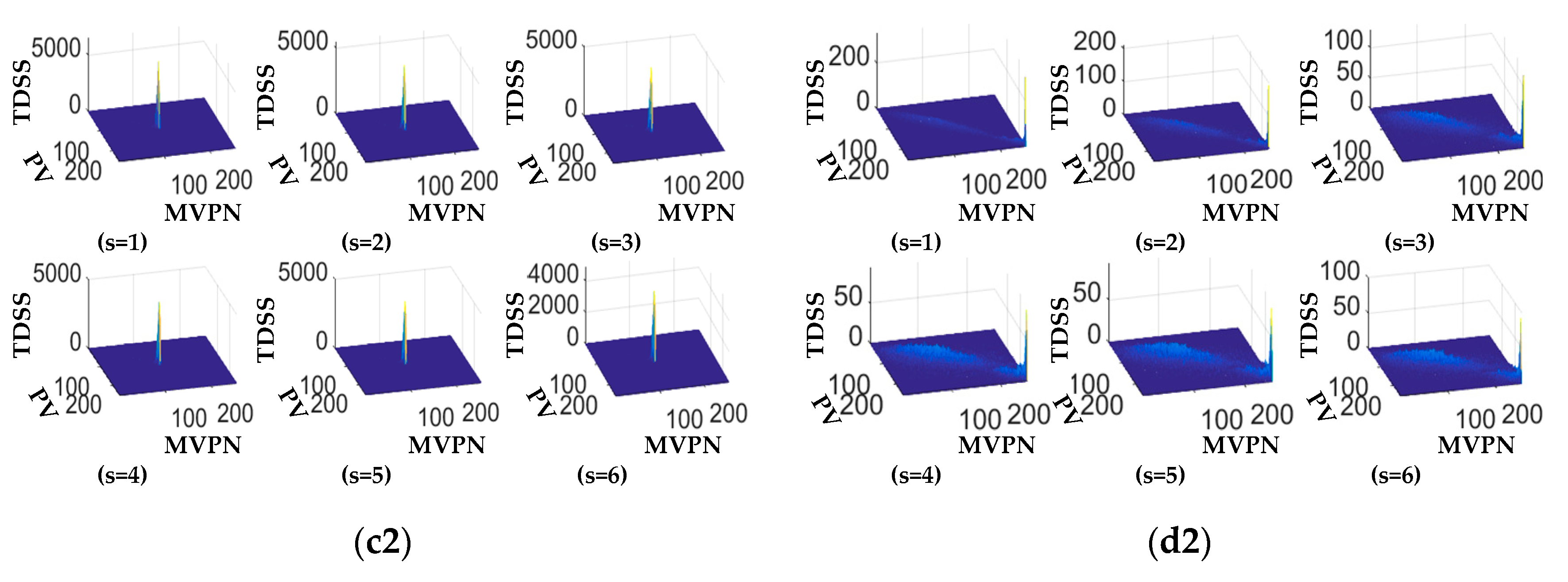
As shown in Figure 5, Figure 5a1–d1 and Figure 5a2–d2 represent the results of the planar mapping model and the geometric mapping model at different mapping levels, respectively. We find that as the radius (from 1 to 6) of different levels of mapping is gradually increased, the degree of dispersion and uniformity of the mapping models of experimental images gradually increases and tends to be stable after the mapping radius is equal to or larger than a certain radius, which we here observed is approximately 5. This finding also confirms the existing issues in the single geometrical mapping model, i.e., the single-level-mapping-model-based GME model reflects attribute information from a certain level contained in images and might neglect some important information, such as the information of multilevel and multiscale characteristics of spatial structures, so that measurement results are too one-sided to be reliable.
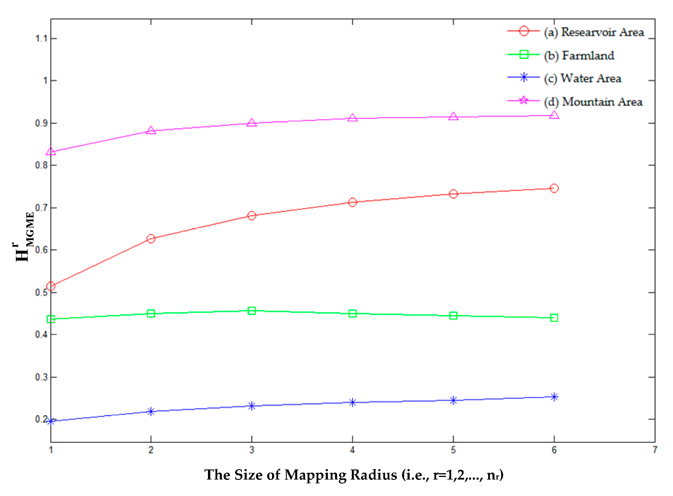
In Table 1, the related measurement results of Figure 5a–d obtained by the MGME and traditional image entropy methods are listed, and Figure 6 describes the distribution curve of the corresponding results using different mapping radii in the proposed method. Through comparative analysis, we find that compared with results from other experimental images (i.e., Figure 5a–c), the measurement results (from 0.832 to 0.917) of the different mapping radii in Figure 5d are all maximized. This finding is because of all the sample images, its spatial structure is the most complicated, and the degree of dispersion and uniformity of brightness values of the ground scene within it are also the largest. As a result, the corresponding uncertain information is the greatest of all the images, i.e., the amount of information is also the largest.
Another meaningful finding we observed from Table 1 is that the image (Figure 5a) of a reservoir area in comparison with the other three experimental images (Figure 5b–d) is mainly composed of three types of ground objects (i.e., water area, town area, and farmland) but contains other types of land cover (e.g., trees, roads, and grass) within some small areas. Since the difference in the abovementioned ground objects is considerably large, this makes the multilevel and multiscale characteristics of spatial structures in Figure 5a even more obvious. An identical conclusion was obtained using the standard deviation () values of the MGME vector set of experimental images, where the (0.079) of Figure 5a in comparison with other images is the largest, and the (0.030) of Figure 5d is the second largest. Furthermore, we can see that the distribution of farmland (Figure 5b) is regular, the multilevel characteristics of spatial structures of Figure 5c in comparison with Figure 5b are relatively distinct, i.e., the (0.019) of Figure 5c is larger than the (0.007) of Figure 5b.
By comparing and analyzing experimental results from different types of images, it can be found that as the mapping radius of different levels is gradually increased, the measurement results of these images also become gradually larger and then tend to stabilize. These results show that the MGME model in comparison with the single-level GME model can reflect much more attribute feature information contained in the images. Especially for images that contain many different object types, the of the vector set from the multilevel GME can reflect, to some degree, the difference in the local spatial structural features of images. In other words, more categories of ground objects lead to a larger difference between different ground objects or a more disordered spatial distribution and greater (also called volatility) of the MGEM vector set. On the basis of our findings, it can be concluded that the multilevel mapping strategy proposed in this paper is feasible and valid.
4.2. Experiment 2
This section is used to further validate the necessity of adopting a multilevel mapping strategy to evaluate the feature information of images. Furthermore, we discuss and analyze the application prospects of this strategy. Experimental images were mainly obtained from UAV images of different local areas in the districts of the lower and middle reaches of the Yellow River in 2015, in Kaifeng. The images primarily contain water areas, trees, and other land covers, such as grass, footpaths, and pavilions, as shown in Figure 7.
Notably, we can see from Figure 7a–d that the object types contained in experimental images are approximately changed from a single object (water area) to mixed objects (water area and trees). Meanwhile, as the proportion of trees increases within an area of equal size, the amount of uncertain information in images is gradually increased as a whole, and the degree of complexity of the spatial distribution and organizational structure of the images increases as well.
Subsequently, we used the results of traditional image entropy and the MGME model to contrast and analyze the experimental data in this section from a quantitative perspective. The results are shown in Table 2.
As can be seen from Table 2, in the images from Figure 7c,d, the and of Figure 7d are all lower than the corresponding calculated results of Figure 7c. Nevertheless, as the radius of the mapping model gradually increases (i.e., r > 1), the (e.g., , , and ) of Figure 7d become larger than the results of Figure 7c, as shown in Figure 8. This result is consistent with subjective judgment of human visual perception. This result also indicates that the MGME method in comparison with traditional image entropy and a single-level GME model can, to a certain extent, better evaluate the information content and reflect the multilevel characteristics of spatial structure in images.
By and large, the values of experimental images gradually become larger. The values of Figure 7c,d are equal to 0.027 and 0.053, respectively. These values confirm that the spatial structure and organization distribution of Figure 7d (including water area, trees, grass, and pathway) in comparison with Figure 7c is more complex. The value of Figure 7a equals 0.001, which is approximately zero. This finding is consistent with the fact that this image contains a single type of ground object (i.e., water area).
The inconsistent relationship between sizes and measurement results in Figure 7c,d at different mapping levels (e.g., r = 1,2) fully shows that it is quite necessary to use a multilevel mapping strategy to evaluate the feature information. A multilevel mapping strategy can validly eliminate the influence of the one-sidedness of a single mapping model on the results of feature information. Furthermore, the MGME model proposed in this paper can validly reflect, to some degree, the information on the spatial structural features in images. We further attempt to use this method to explore and study local spatial correlations and multiscale characteristics of spatial structures in images.
5. Conclusions
In this study, we presented a multilevel-mapping-strategy-based approach for evaluating the information content of images. Based on the neighborhood two-dimensional grayscale array, the multilevel geometrical mapping entropy (MGME) model is developed by incorporating the ideas of scatterplot matrices and multilevel mapping into the modeling process. Here, we use different types of objects from experimental images to validate the performance of the proposed method, i.e., reservoir area, farmland, water area, and mountainous area. The experimental results in experiment 1 and experiment 2 indicate that the multilevel mapping strategy in comparison with a single level mapping model can validly characterize much more attribute feature information while overcoming the adverse influence of the single-level GME model on the accurate evaluation of feature information in images. Moreover, we also find that the Std of the MGME vector can effectively reflect, to some extent, the multilevel characteristics of spatial structures contained in images. That is, this approach can provide a new pathway for research on the spatial structural features of images, such as spatial autocorrelation.
In the future, we will also further develop the method proposed so as to enhance its reliability and accuracy. The maximum radius setting/selection of the MGME model for images with different spatial structure deserves focused research. The proposed calculated approach can be extended to different types of remote sensing images (e.g., multispectral, infrared images). Furthermore, we can explore and investigate the performance of this method when it is applied to practical image processing and other applications, such as data screening and data mining.
Author Contributions
Shimin Fang conceived and designed the methodology; Shimin Fang processed the experimental data, implemented all experiments, and wrote the manuscript; Xiaoguang Zhou supervised the research; Xiaoguang Zhou and Jing Zhang provided some useful suggestions, read, and helped to revise the manuscript.
Funding
This research was funded by the Natural Key Research and Development Program of China (Grant No. 2016YFB05140307).
Acknowledgments
The author is gratefully acknowledged for advice and support provided. We would also thank the anonymous reviewers whose insightful comments improved this letter.
Conflicts of Interest
The authors declare that they have no conflict of interest.
References
- Alonso, K.; Datcu, M. Accelerated probabilistic learning concept for mining heterogeneous earth observation images. IEEE J. Sel. Top. Appl. Earth Obs. Remote Sens. 2015, 8, 3356–3371. [Google Scholar] [CrossRef]
- Ma, Y.; Wu, H.; Wang, L.; Huang, B.; Ranjan, R.; Zomaya, A.; Jie, W. Remote sensing big data computing: Challenges and opportunities. Future Generati. Comput. Syst. 2015, 51, 47–60. [Google Scholar] [CrossRef]
- Chen, J.; Dowman, I.; Li, S.; Li, Z.; Madden, M.; Mills, J.; Paparoditis, N.; Rottensteiner, F.; Sester, M.; Toth, C. Information from imagery: ISPRS scientific vision and research agenda. ISPRS J. Photogr. Remote Sens. 2016, 115, 3–21. [Google Scholar] [CrossRef] [Green Version]
- Benediktsson, J.A.; Chanussot, J.; Moon, W.M. Very high-resolution remote sensing: Challenges and opportunities [point of view]. Proc. IEEE 2012, 100, 1907–1910. [Google Scholar] [CrossRef]
- Kitchin, R. Big data and human geography: Opportunities, challenges and risks. Dialog. Hum. Geogr. 2013, 3, 262–267. [Google Scholar] [CrossRef]
- Li, Z.; Shen, H.; Li, H.; Xia, G.; Gamba, P.; Zhang, L. Multi-feature combined cloud and cloud shadow detection in GaoFen-1 wide field of view imagery. Remote Sens. Environ. 2017, 191, 342–358. [Google Scholar] [CrossRef] [Green Version]
- Johnson, B.; Xie, Z. Unsupervised image segmentation evaluation and refinement using a multiscale approach. ISPRS J. Photogr. Remote Sens. 2011, 66, 473–483. [Google Scholar] [CrossRef]
- Xie, L.; Li, G.; Xiao, M.; Peng, L. Novel classification method for remote sensing images based on information entropy discretization algorithm and vector space model. Comput. Geosci. 2016, 89, 252–259. [Google Scholar] [CrossRef]
- Ma, C.; Wei, X.; Fu, C.; Liu, J.; Wei, L. A Content-Based Remote Sensing Image Change Information Retrieval Model. ISPRS Int. J. Geo-Inform. 2017, 6, 310. [Google Scholar] [CrossRef]
- Erus, G.; Loménie, N. How to involve structural modeling for cartographic object recognition tasks in high-resolution satellite images? Pattern Recognit. Lett. 2010, 31, 1109–1119. [Google Scholar] [CrossRef] [Green Version]
- Huang, X.; Zhang, L.; Li, P. Classification and extraction of spatial features in urban areas using high-resolution multispectral imagery. IEEE Geosci. Remote Sens. Lett. 2007, 4, 260–264. [Google Scholar] [CrossRef]
- Qin, K.; Chen, Y.; Gan, S.; Feng, X.; Ren, W. Review on methods of spatial structural feature modeling of high resolution remote sensing images. J. Image Gr. 2013, 18, 1055–1064. [Google Scholar]
- Chen, Y.; Qin, K.; Gan, S.; Wu, T. Structural feature modeling of high-resolution remote sensing images using directional spatial correlation. IEEE Geosci. Remote Sens. Lett. 2014, 11, 1727–1731. [Google Scholar] [CrossRef]
- Quartulli, M.; Olaizola, I.G. A review of EO image information mining. ISPRS J. Photogr. Remote Sens. 2013, 75, 11–28. [Google Scholar] [CrossRef] [Green Version]
- Tang, X.; Zhang, X.; Liu, F.; Jiao, L. Unsupervised deep feature learning for remote sensing image retrieval. Remote Sens. 2018, 10, 1243. [Google Scholar] [CrossRef]
- Daschiel, H.; Datcu, M. Information mining in remote sensing image archives: System evaluation. IEEE Trans. Geosci. Remote Sens. 2005, 43, 188–199. [Google Scholar] [CrossRef]
- Datcu, M.; Seidel, K.; D′Elia, S.; Marchetti, P. Knowledge-driven information mining in remote-sensing image archives. ESA Bull. 2002, 110, 26–33. [Google Scholar]
- Zhou, W.; Newsam, S.; Li, C.; Shao, Z. PatternNet: A benchmark dataset for performance evaluation of remote sensing image retrieval. ISPRS J. Photogr. Remote Sens. 2018, 145, 197–209. [Google Scholar] [CrossRef] [Green Version]
- Datcu, M.; Daschiel, H.; Pelizzari, A.; Quartulli, M.; Galoppo, A.; Colapicchioni, A.; Pastori, M.; Seidel, K.; Marchetti, P.G.; d′Elia, S. Information mining in remote sensing image archives: System concepts. IEEE Trans. Geosci. Remote Sens. 2003, 41, 2923–2936. [Google Scholar] [CrossRef]
- Tsai, D.-Y.; Lee, Y.; Matsuyama, E. Information entropy measure for evaluation of image quality. J. Digit. Imaging 2008, 21, 338–347. [Google Scholar] [CrossRef]
- Hu, L.; He, Z.; Liu, J.; Zheng, C. Method for measuring the information content of terrain from digital elevation models. Entropy 2015, 17, 7021–7051. [Google Scholar] [CrossRef]
- Malila, W.A. Comparison of the information contents of Landsat TM and MSS data. Photogr. Eng. Remote Sens. 1985, 51, 1449–1457. [Google Scholar]
- Sun, J.; Zhang, X.; Cui, J.; Zhou, L. Image retrieval based on color distribution entropy. Pattern Recognit. Lett. 2006, 27, 1122–1126. [Google Scholar] [CrossRef]
- Li, Z.; Liu, Q.; Gao, P. Entropy-based cartographic communication models: Evolution from special to general cartographic information theory. Acta. Geod. Cartogr. Sin. 2016, 45, 757–767. [Google Scholar]
- Chen, T.M.; Staelin, D.H.; Arps, R.B. Infornation content analysis of landsat image data for compression. IEEE Trans. Geosci. Remote Sens. 1987, GE-25, 499–501. [Google Scholar] [CrossRef]
- Lin, Z.; Zhang, Y. Measurement of information and uncertainty of remote sensing and GIS data. Geomat. Inf. Sci. Wuhan Univ. 2006, 31, 569–572. [Google Scholar]
- Zhang, Y.; Zhang, J. Measure of information content of remotely sensed images accounting for spatial correlation. Acta Geod. Cartogr. Sin. 2015, 44, 1117–1124. [Google Scholar]
- Blacknell, D.; Oliver, C. Information content of coherent images. J. Phys. D Appl. Phys. 1993, 26, 1364. [Google Scholar] [CrossRef]
- Moore, R.K. Tradeoff between picture element dimensions and noncoherent averaging in side-looking airborne radar. IEEE Trans. Aerosp. Electron. Syst. 1979, AES-15, 697–708. [Google Scholar] [CrossRef]
- Narayanan, R.M.; Desetty, M.; Reichenbach, S. Effect of spatial resolution on information content characterization in remote sensing imagery based on classification accuracy. Int. J. Remote Sens. 2002, 23, 537–553. [Google Scholar] [CrossRef]
- Román-Roldán, R.; Quesada-Molina, J.; Martínez-Aroza, J. Multiresolution-information analysis for images. Signal Process. 1991, 24, 77–91. [Google Scholar] [CrossRef]
- Price, J.C. Comparison of the information content of data from the landsat-4 thematic mapper and the multispectral scanner. IEEE Trans. Geosci. Remote Sens. 1984, GE-22, 272–281. [Google Scholar] [CrossRef]
- Verde, N.; Mallinis, G.; Tsakiri-Strati, M.; Georgiadis, C.; Patias, P. Assessment of radiometric resolution impact on remote sensing data classification accuracy. Remote Sens. 2018, 10, 1267. [Google Scholar] [CrossRef]
- Gao, P.; Zhang, H.; Li, Z. A hierarchy-based solution to calculate the configurational entropy of landscape gradients. Landsc. Ecol. 2017, 32, 1133–1146. [Google Scholar] [CrossRef]
- Cushman, S.A. Calculating the configurational entropy of a landscape mosaic. Landsc. Ecol. 2016, 31, 481–489. [Google Scholar] [CrossRef]
- Cushman, S. Calculation of configurational entropy in complex landscapes. Entropy 2018, 20, 298. [Google Scholar] [CrossRef]
- Gao, P.; Zhang, H.; Li, Z. An efficient analytical method for computing the Boltzmann entropy of a landscape gradient. Trans. GIS 2018, 22, 1046–1063. [Google Scholar] [CrossRef]
- Razlighi, Q.R.; Rahman, M.T.; Kehtarnavaz, N. Fast computation methods for estimation of image spatial entropy. J. Real-Time Image Process. 2011, 6, 137–142. [Google Scholar] [CrossRef]
- Benz, U.C.; Hofmann, P.; Willhauck, G.; Lingenfelder, I.; Heynen, M. Multi-resolution, object-oriented fuzzy analysis of remote sensing data for GIS-ready information. ISPRS J. Photogr. Remote Sens. 2004, 58, 239–258. [Google Scholar] [CrossRef]
- Tobler, W.R. A computer movie simulating urban growth in the Detroit region. Econ. Geogr. 1970, 46, 234–240. [Google Scholar] [CrossRef]
- Henebry, G.M. Detecting change in grasslands using measures of spatial dependence with Landsat TM data. Remote Sens. Environ. 1993, 46, 223–234. [Google Scholar] [CrossRef]
- Wulder, M.; Boots, B. Local spatial autocorrelation characteristics of remotely sensed imagery assessed with the Getis statistic. Int. J. Remote Sens. 1998, 19, 2223–2231. [Google Scholar] [CrossRef]
- Itti, L.; Koch, C. Computational modelling of visual attention. Nat. Rev. Neurosci. 2001, 2, 194. [Google Scholar] [CrossRef] [PubMed]
- Pelizzari, A.; Descargues, V.; Datcu, M.P. Visual information mining in remote sensing image archives. In Image and Signal Processing for Remote Sensing VII; International Society for Optics and Photonics; SPIE: Philadelphia, PA, USA, 2002; pp. 241–251. [Google Scholar]
- Cheng, H.D.; Sun, Y. A hierarchical approach to color image segmentation using homogeneity. IEEE Trans. Image Process. 2000, 9, 2071–2082. [Google Scholar] [PubMed]
- Puissant, A.; Hirsch, J.; Weber, C. The utility of texture analysis to improve per—pixel classification for high to very high spatial resolution imagery. Int. J. Remote Sens. 2005, 26, 733–745. [Google Scholar] [CrossRef]
- Shannon, C.E. A mathematical theory of communication. Bell Syst. Tech. J. 1948, 27, 379–423. [Google Scholar] [CrossRef]
- Li, Z.; Huang, P. Quantitative measures for spatial information of maps. Int. J. Geogr. Inf. Sci. 2002, 16, 699–709. [Google Scholar] [CrossRef]
- Chen, P.; Shi, W. Measuring the spatial relationship information of multi-layered vector data. ISPRS Int. J. Geo-Inf. 2018, 7, 88. [Google Scholar] [CrossRef]
- Uchida, S.; Tsai, D.Y. Evaluation of radiographic images by entropy: Application to development process. Jpn. J. Appl. Phys. 1978, 17, 2029. [Google Scholar] [CrossRef]
- Zhang, Q.; Zhang, P.; Xiao, Y. A Modeling and measurement approach for the uncertainty of features extracted from remote sensing images. Remote Sens. 2019, 11, 1841. [Google Scholar] [CrossRef]
- Datcu, M.; Seidel, K.; Walessa, M. Spatial information retrieval from remote-sensing images. I. Information theoretical perspective. IEEE Trans. Geosci. Remote Sens. 1998, 36, 1431–1445. [Google Scholar] [CrossRef]
- Quweider, M. Spatial entropy-based cost function for gray and color Image segmentation with dynamic optimal partitioning. Int. J Comput. Sci. Netw. Secur. 2012, 12, 64. [Google Scholar]
- Akçay, H.G.; Aksoy, S. Automatic detection of geospatial objects using multiple hierarchical segmentations. IEEE Trans. Geosci. Remote Sens. 2008, 46, 2097–2111. [Google Scholar] [CrossRef]
- Bruzzone, L.; Carlin, L. A multilevel context-based system for classification of very high spatial resolution images. IEEE Trans. Geosci. Remote Sens. 2006, 44, 2587–2600. [Google Scholar] [CrossRef]
- Elmqvist, N.; Dragicevic, P.; Fekete, J.D. Rolling the dice: Multidimensional visual exploration using scatterplot matrix navigation. IEEE Trans. Vis. Comput. Gr. 2008, 14, 1539–1148. [Google Scholar] [CrossRef]
- Sedlmair, M.; Munzner, T.; Tory, M. Empirical guidance on scatterplot and dimension reduction technique choices. IEEE Trans. V. Comput. Gr. 2013, 19, 2634–2643. [Google Scholar] [CrossRef]
- Touchette, P.E.; MacDonald, R.F.; Langer, S.N. A scatter plot for identifying stimulus control of problem behavior. J. Appl. Behave. Anal. 1985, 18, 343–351. [Google Scholar] [CrossRef]
- Bovolo, F. A multilevel parcel-based approach to change detection in very high resolution multitemporal images. IEEE Geosci. Remote Sens. Lett. 2008, 6, 33–37. [Google Scholar] [CrossRef]
- Yang, Y.; Newsam, S. Geographic image retrieval using local invariant features. IEEE Trans. Geosci. Remote Sens. 2013, 51, 818–832. [Google Scholar] [CrossRef]
- Franklin, S.; Wulder, M.; Lavigne, M. Automated derivation of geographic window sizes for use in remote sensing digital image texture analysis. Comput. Geosci. 1996, 22, 665–673. [Google Scholar] [CrossRef]
- Li, D.; Wang, S.; Li, D. Spatial Data Mining Theories and Application; Springer: Beijing, China, 2015. [Google Scholar]
Figure 1.
Neighborhood window of the target pixel.

Figure 2.
Description of spatial structural characteristics.

Figure 3.
Sketch map of the different-level mapping strategy.

Figure 4.
Block diagram of the multilevel geometrical mapping entropy (MGME) model.

Figure 5.
The scatter-mapping-strategy-based results with different levels, (a–d) experimental images; (a1–d1) planar mapping model; (a2–d2) geometrical mapping model.
Figure 5.
The scatter-mapping-strategy-based results with different levels, (a–d) experimental images; (a1–d1) planar mapping model; (a2–d2) geometrical mapping model.


Figure 6.
The distribution curve of the MGME results using different mapping radii.

Figure 7.
UAV images of different local areas used in experiment 2.

Figure 8.
The distribution curve of the MGME results using different mapping radii.


Table 1.
Results of traditional image entropy and the MGME model.
| Experimental Images | Traditional Method | Multilevel Geometrical Mapping Entropy | |||||||||
|---|---|---|---|---|---|---|---|---|---|---|---|
| r = 1 | r = 2 | r = 3 | r = 4 | r = 5 | r = 6 | ||||||
| (a) Reservoir Area | 7.193 | 0.514 | 0.626 | 0.681 | 0.713 | 0.732 | 0.745 | 0.669 | 0.678 | 4.011 | 0.079 |
| (b) Farmland | 6.432 | 0.436 | 0.450 | 0.456 | 0.450 | 0.445 | 0.440 | 0.446 | 0.460 | 2.667 | 0.007 |
| (c) Water Area | 4.425 | 0.195 | 0.218 | 0.231 | 0.239 | 0.245 | 0.253 | 0.230 | 0.232 | 1.381 | 0.019 |
| (d) Mountain Area | 7.827 | 0.832 | 0.882 | 0.899 | 0.911 | 0.915 | 0.917 | 0.893 | 0.894 | 5.356 | 0.030 |
Table 2.
Results of traditional image entropy and the MGME model.
| Experimental Images | Traditional Method | Multilevel Geometrical Mapping Entropy | |||||||||
|---|---|---|---|---|---|---|---|---|---|---|---|
| r = 1 | r = 2 | r = 3 | r = 4 | r = 5 | r = 6 | ||||||
| (a) Local Area 1 | 3.097 | 0.030 | 0.032 | 0.032 | 0.032 | 0.032 | 0.032 | 0.032 | 0.032 | 0.190 | 0.001 |
| (b) Local Area 2 | 4.425 | 0.195 | 0.218 | 0.231 | 0.239 | 0.245 | 0.253 | 0.230 | 0.232 | 1.381 | 0.019 |
| (c) Local Area 3 | 5.595 | 0.354 | 0.403 | 0.421 | 0.427 | 0.430 | 0.429 | 0.411 | 0.412 | 2.464 | 0.027 |
| (a) Local Area 1 | 5.550 | 0.342 | 0.442 | 0.458 | 0.480 | 0.490 | 0.496 | 0.448 | 0.454 | 2.688 | 0.053 |
© 2019 by the authors. Licensee MDPI, Basel, Switzerland. This article is an open access article distributed under the terms and conditions of the Creative Commons Attribution (CC BY) license (http://creativecommons.org/licenses/by/4.0/).
Share and Cite
MDPI and ACS Style
Fang, S.; Zhou, X.; Zhang, J. A Multilevel Mapping Strategy to Calculate the Information Content of Remotely Sensed Imagery. ISPRS Int. J. Geo-Inf. 2019, 8, 464. https://0-doi-org.brum.beds.ac.uk/10.3390/ijgi8100464
AMA Style
Fang S, Zhou X, Zhang J. A Multilevel Mapping Strategy to Calculate the Information Content of Remotely Sensed Imagery. ISPRS International Journal of Geo-Information. 2019; 8(10):464. https://0-doi-org.brum.beds.ac.uk/10.3390/ijgi8100464
Chicago/Turabian StyleFang, Shimin, Xiaoguang Zhou, and Jing Zhang. 2019. "A Multilevel Mapping Strategy to Calculate the Information Content of Remotely Sensed Imagery" ISPRS International Journal of Geo-Information 8, no. 10: 464. https://0-doi-org.brum.beds.ac.uk/10.3390/ijgi8100464
Note that from the first issue of 2016, this journal uses article numbers instead of page numbers. See further details here.