An Adaptive Construction Method of Hierarchical Spatio-Temporal Index for Vector Data under Peer-to-Peer Networks

Abstract

Spatio-temporal indexing is a key technique in spatio-temporal data storage and management. Indexing methods based on spatial filling curves are popular in research on the spatio-temporal indexing of vector data in the Not Relational (NoSQL) database. However, the existing methods mostly focus on spatial indexing, which makes it difficult to balance the efficiencies of time and space queries. In addition, for non-point elements (line and polygon elements), it remains difficult to determine the optimal index level. To address these issues, this paper proposes an adaptive construction method of hierarchical spatio-temporal index for vector data. Firstly, a joint spatio-temporal information coding based on the combination of the partition and sort key strategies is presented. Secondly, the multilevel expression structure of spatio-temporal elements consisting of point and non-point elements in the joint coding is given. Finally, an adaptive multi-level index tree is proposed to realize the spatio-temporal index (Multi-level Sphere 3, MLS3) based on the spatio-temporal characteristics of geographical entities. Comparison with the XZ3 index algorithm proposed by GeoMesa proved that the MLS3 indexing method not only reasonably expresses the spatio-temporal features of non-point elements and determines their optimal index level, but also avoids storage hotspots while achieving spatio-temporal retrieval with high efficiency.

1. Introduction

With the development of Internet technologies, peer-to-peer (P2P) networks are currently receiving considerable interest as they provide a decentralized architecture in which the shared resources on one node can be directly accessed by other peers without passing through intermediate entities [1]. In recent years, P2P communication software has become the mainstream solution for big data storage and management in smart city construction for its excellent characteristics for processing spatio-temporal data, such as full distribution, high availability, high throughput, and linear expansibility [2,3]. During this process, the efficient index algorithms in P2P networks are facing serious challenges. For traditional master-slave architecture system, the efficiency of the whole network can be improved by expanding the performance of the hardware of central server. However, this strategy is difficult to apply to P2P networks because data resources in P2P networks are randomly distributed in different nodes with equal status and some of them have low performance. Hence, it is an urgent need to find a high-efficiency global indexing structure in P2P networks, which can quickly locate the node where the data are stored and the global query performance will not be affected by the data update of local nodes.

The volume of available spatio-temporal data have increased tremendously in the last few years. Such data includes but is not limited to: taxi trajectory data, social network data, remote-sensing image data, weather maps, and more. Beside the huge achieved volume of the data, space and time are two fundamental characteristics that raise the demand for processing spatio-temporal data [4]. Even though existing big spatio-temporal data-management systems are efficient for time or spatial operations by constructing a time index or a spatial index, nonetheless these systems with single index or sequencing structure suffer when they are processing spatio-temporal queries, e.g., “find taxis in nanjing road during the last two months”. If simply sequencing a spatial index and a time index, no matter which query is done first, it always results in scanning through a lot of irrelevant data to the query answer when the data set is great and complex. In addition, this kind of query is usually unaware of the spatio-temporal granularity properties of the objects, especially when they are routinely achieved on a large scale [4]. The construction of an efficient spatio-temporal index has been of great interest for big data storage and management in geographic information system (GIS) [5,6] in recent research. For distributed Not Relational (NoSQL) databases, spatio-temporal index research can be divided into two categories:

• Studies focused on improving or expanding traditional spatial index (QuadTree, R-Tree, Grid index, etc.) for distributed environments [7,8,9,10]. For example, as an extended MapReduce framework, SpatialHadoop provides a generic global indexing algorithm which was used to implement Grid, R-tree, R+-tree, Quad-tree, and k-dimensional (KD) tree based partitioning [11]. Spatio-temporal (ST) Hadoop, which is a comprehensive extension to Hadoop and SpatialHadoop, takes the advantages of applying the aforementioned spatial bulk loading techniques that are already implemented in SpatialHadoop and spatiotemporally loads and divides data across computation nodes, which result in achieving orders of magnitude better performance than Hadoop and SpatialHadoop [4]. GeoSpark also provides uniform grid, R-tree, Quad-Tree, and KDB-Tree (the combination of KD-tree and B-tree) spatial data indexing algorithm and it builds local spatial indexes on each Spark data partition to speed up the local computation [12]. Such index structure always need long constructing time, high updating cost and the index consistency is difficult to maintain, hence it is not suitable for the spatio-temporal data which updated frequently in distributed environments.
• Studies focused on constructing an index based on space-filling curves (SFCs; Z-Order, Hilbert, Google S2, etc.). Fox et al. [13] proposed a spatio-temporal index structure that uses a GeoHash string to identify the spatial information and interleaves the time attribute string to form the index key value. Le et al. [14] proposed a spatial index method by combining R-Tree and Geohash. Google implemented a spatial index called S2 by combining a quadtree and Hilbert curve, enabling the expression of multi-level spatial elements [15,16]. GeoMesa [17], a popular open source project, involves implementing an extended Z-ordering (XZ-ordering) spatio-temporal indexing method based on Z-order [18]. In this approach, XZ sorting is utilized to express spatial information at arbitrary resolution, and the query performance does not deteriorate with increasing resolution [19,20]. Moreover, Eldawy et al. [21] extend the traditional spatial index by introducing Z-curve and Hilbert curve partitioning techniques in SpatialHadoop. The SFC-based strategy can better describe the spatial continuity characteristics of spatio-temporal data due to its spatial agglomeration characteristics [22,23]. Therefore, this approach has been widely used in spatio-temporal index studies in recent years. However, in the existing SFC index-based research, the spatial and temporal attributes have generally been separated, which has made it difficult to take into account the efficiencies of temporal and spatial queries simultaneously. In addition, for line and polygon elements with different geographic ranges, the efficiencies and accuracies of queries are closely related to the index level used, and a means of achieving a reasonable spatio-temporal expression and determining a practical index level has not yet been identified.

As a NoSQL database in a P2P network, Apache Cassandra database [24,25] has shown great advantages in the management of massive data with dynamic growth in GIS. However, the spatio-temporal management of NoSQL databases, such as vector data, has rarely been researched [26,27]. Although GeoMesa provides the XZ3 spatio-temporal index method, which can be used in P2P networks, its efficiency for spatial data retrieval requires improvement due to its fixed level and the poor continuity of its expressions of non-point elements. This paper focuses on the global spatio-temporal joint indexing of vector data under the P2P network by proposing a multilevel expression structure of spatio-temporal elements and an optimal index hierarchy determination algorithm considering the time granularity and spatial distribution feature of input files in the NoSQL database based on the S2 spatial index, which can achieve efficient spatio-temporal queries and stable query performance as well as a low index-maintaining cost.

The remainder of this article is organized as follows. Section 2 describes the two main spatio-temporal indexing methods and their limitations in vector data management in P2P networks. Section 3 presents an adaptive construction method of hierarchical spatio-temporal index. Section 4 discusses a series of experiments that was conducted to validate the reliability and efficiency of the proposed method. Finally, Section 5 summarizes the conclusions and topics requiring future work.

2. Related Work

2.1. XZ3 Spatio-Temporal Index

The XZ3 spatio-temporal index is an extension of XZ ordering [18]. Its basic idea is to combine quadtree with a Z-order curve, interlace GeoHash strings of spatial information with temporal information strings to achieve spatio-temporal information encoding, and distribute data to P2P networks with a random binary number as Row Key. However, this algorithm has some shortcomings in vector data management in P2P networks, which can be summarized as follows:

(1)

The algorithm uses a Z-order curve as an SFC, which has a hopping problem when expressing two-dimensional space. Consequently, the data expressed by proximity coding are not spatially adjacent and leading to a large number of ineffective queries when querying hopping regions.

(2)

When dividing spatial hierarchy, the XZ3 algorithm decides whether to divide further by judging whether the number of cells divided in a hierarchy meets a certain threshold. However, the threshold setting does not fully consider the spatial distribution and density of all the elements in the same layer.

2.2. S2 Spatial Index

The S2 spatio-temporal index was proposed by Google in 2011. The basic idea is to combine a quadtree with a Hilbert curve to geocode a global space, where the quadtree is used to realize multi-level division of the geographical space and the Hilbert curve is used to reduce the two-dimensional space to a one-dimensional space. The construction process consists of five main steps [15,16].

Step 1

Assume a cube surrounding the Earth with radius 1, [−1,1] × [−1,1] × [−1,1], and the center of the earth as the origin. For a certain point or region on the Earth, transform the longitude and latitude coordinates of point p on the minimum bounding rectangle (MBR) surrounding the point or region into three-dimensional coordinates of a cube, p = (lat, lng) => (x, y, z).

Step 2

Project point p onto a certain surface of the cube by following the radial direction, (x, y, z) => (face, u, v), where face represents the number of the surface of the cube, face = {0, 1, 2, 3, 4, 5}, u and v represent the projection coordinates of each surface. Then normalize the projected coordinates u and v to the interval [0, 1].

Step 3

Discrete normalized u and v into i and j, respectively, (face, u, v) => (face, i, j), where i, j ∈ [0, 2ⁿ − 1] denotes the maximum effective bit of the quadtree cell, and n ∈ [0, 30] denotes the depth of the quadtree, which is a hierarchical series.

Step 4

Map the quadtree cell identified by face, i, and j to a Hilbert curve of a certain level, and calculate the corresponding cell ID, (face, i, j) => CellId, where CellId is a 64-bit integer and can uniquely represent a point or region.

S2 can describe spatial continuity characteristics better than XZ3 due to the spatial agglomeration characteristics of the Hilbert curve, so it can achieve better multi-level expression of global elements. However, the following limitations remain.

(1)

Regarding the joint expression of spatio-temporal information, S2 only expresses the spatial information. For spatial geometric elements with multiple time series, an effective means of combining temporal and spatial information has not yet been determined.

(2)

The expression of non-point elements. For line and polygon elements, the spatial scale varies greatly, and for geographic element queries, the spatial span and spatial query mode are both random. It is necessary to take into account both accurate and fast queries in a small range and scanning operation on a large scale. A reasonable method of spatio-temporal expressions is the second limitations.

(3)

The determination of time granularity and optimal hierarchy. In the research on traditional spatial index including regular grid, Quadtree-based grid and R-tree based grid, Belussi et al. [28] pointed out that the efficiencies and accuracies of queries are closely related to spatio-temporal dataset distribution characteristic. Therefore, the lack of a reasonable means of achieving spatio-temporal expression and determining a practical index level according to the spatial and temporal characteristics of elements for the SFC-based index is the third limitation.

To address the aforementioned issues, this paper proposes an adaptive construction method of hierarchical spatio-temporal index for vector data based on the S2 spatial index. Firstly, interleaved joint spatio-temporal information coding based on the combination of the partition and sort key strategies is presented, which makes full use of spatio-temporal granularity properties of the objects to support space and time joint query. Secondly, the multilevel expression structure of spatio-temporal elements consisting of point and non-point elements in the joint coding is given, and this structure will reflect the hierarchical characteristics of spatio-temporal elements. Finally, an adaptive multi-level index tree is proposed to realize the spatio-temporal index, and the optimal index levels are determined by the spatio-temporal dataset distribution characteristic.

3. Methodology

The distributed spatio-temporal index in the NoSQL database is essentially a way of encoding spatio-temporal information in Row Key. Based on the S2 spatial index, this paper proposes an adaptive construction method of hierarchical spatio-temporal index for vector data under P2P networks. We extend the S2 spatial index, which is a Quad tree + Hilbert curve indexing algorithm, by introducing the hierarchical strategy of time and space information and hierarchical dynamic adjustment algorithm according to the spatio-temporal dataset distribution characteristic. The detailed contents of our method are as follows. Firstly, spatio-temporal information is divided according to time granularity and spatial hierarchy. Secondly, mixed encoding is performed based on the refined time granularity and spatial hierarchy, and the codes are stored in Row Key. Thirdly, an adaptive multi-level index tree is proposed to construct the spatio-temporal index (Multi-level Sphere 3, MLS3) based on the spatio-temporal characteristics of geographical entities. Finally, according to a consistent hash algorithm, Row Key is hashed to achieve distributed storage of spatio-temporal data in the P2P network, as shown in Figure 1.

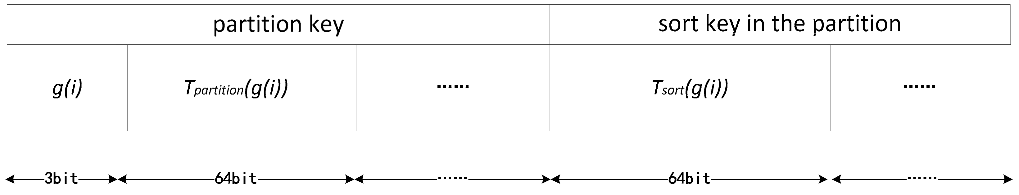
3.1. Joint Coding of Spatio-Temporal Information

The notion of a table in NoSQL database, such as Cassandra, is different from the notion of a table in a relational database. In general, each partition in a table has a unique partition key and each row in a partition may optionally have a unique sort key (clustering key). The combination of the partition and sort key is defined as the compound key, which can uniquely identifies a row in a table. The advantage of the compound keys is that they can accelerate the efficiency of data retrieval and ensures that the data directly read from the disk is the ordered data satisfying the query conditions [27]. We proposed a joint spatio-temporal information coding based on compound keys. The partition key is used to describe the large granularity spatio-temporal, so as to locate quickly the storage node where the data is stored in the P2P networks, and the sort key is used to describe the small granularity spatio-temporal, so as to realize the sequential retrieval of data in the storage node.

3.1.1. Time Information Coding

The time information is divided into six levels according to the data update period or sampling frequency. The time granularity ranges from seconds to years and is marked as g_i (i = 0, 1, …, 5), as shown in

Table 1. Time information coding.

Time Granularity	Partition Key	Partition Key Time Format	Sort Key	Sort Key Time Format
0	Year	yyyy	Month-Day Hour-Minute	MMdd hh:mm:ss
1	Year-Month	yyyyMM	Day Hour-Minute	dd hh:mm:ss
2	Year-Month-Day	yyyyMMdd	Hour-Minute-Second	hh:mm:ss
3	Year-Month-Day Hour	yyyyMMdd hh	Minute-Second	mm:ss
4	Year-Month-Day Hour-Minute	yyyyMMdd hh:mm	Second	ss
5	Year-Month-Day Hour-Minute-Second	yyyyMMdd hh:mm:ss	—	—

.

Supposing T_base is the starting point, T_current is the number of milliseconds from the current time to T_base (under time granularity g₅), i.e., T_current = T(g₅) − T_base. Take the integer part of the current time corresponding to the time granularity in Table 1 as the partition key, named T_partition(g_i) and the sort key T_sort(g_i) = T_current − T_partition(g_i). The coding of time information part in the Row Key is shown in Figure 2.

3.1.2. Spatial Information Coding

According to the basic idea of constructing S2, each spatial element could be identified by one or more cells containing the element. Taking the line element as an example, as shown in Figure 3, the cell set of the line element (red solid line) passing through the first level L₁ was (0, 2, 3), that of the line element passing through the second level L₂ was (00, 02, 03, 22, 23, 30, 31), and that of the line element passing through the third level L₃ was (001, 002, 020, 022, 023, 031, 220, 231, 232, 303, 310, 311).

In this study, the S2 spatial index was extended to establish a quadtree + Hilbert curve with finite depth (quadruple Height ≤ depth threshold Height_thresh), and the spatial information was represented by multi-level Hilbert coding. For vector objects, supposing its hierarchy is limited to L_m–L_n (0 ≤ m < n ≤ 30), then taking the code of spatial information at the lower m level as the partition key, and the sorting key is the code at the higher n level. The coding of spatial information part in Row Key is shown in Figure 4.

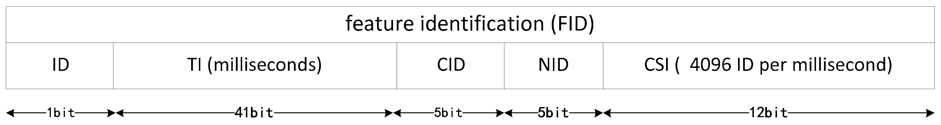
3.1.3. Feature Identification Information Coding

The feature identification (FID) includes five parts: Identification (ID), Timestamp Identification (TI), Cluster Identification (CID), Node Identification (NID), and Counting Sequence Identification (CSI), as shown in Figure 5. The FID was generated using the SnowFlake algorithm by Twitter [29], which was sorted by ID value in general and further identified by CID and NID to ensure that no duplicate FID could be generated in the entire P2P network.

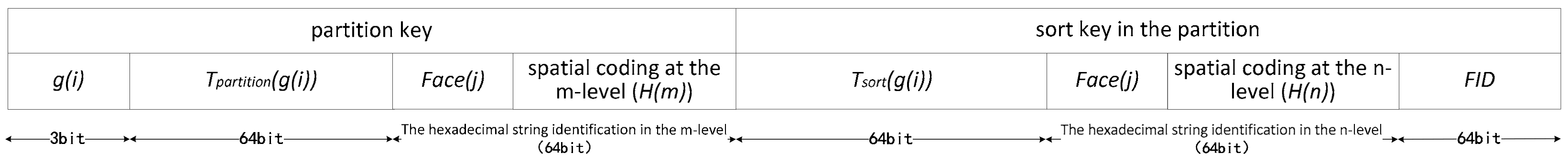
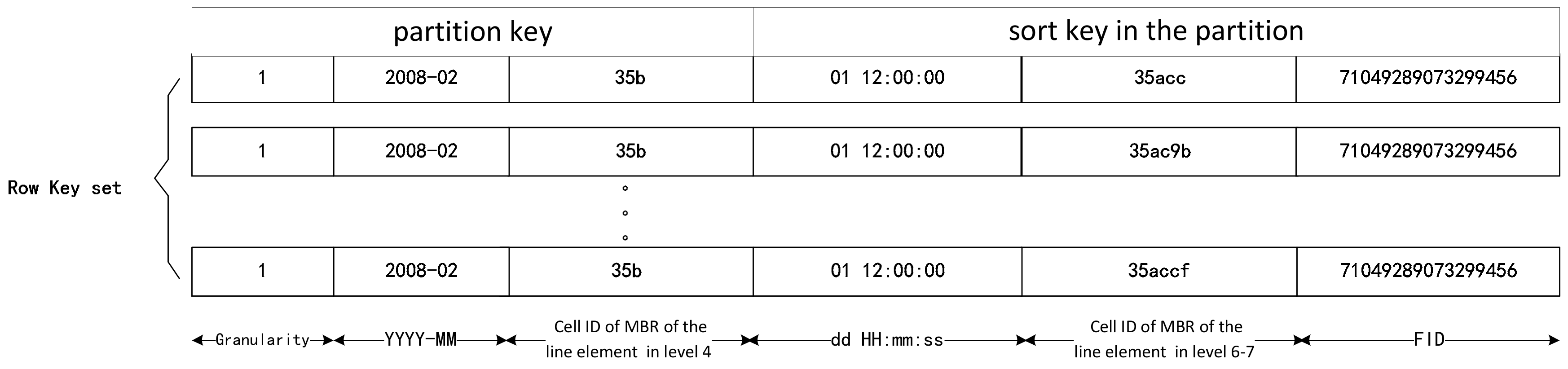
3.1.4. Organization of Row Key Coding

Integrating the aforementioned time coding, spatial coding, and FID to form a unified structure of Row Key coding, the organization mode is as follows. (1) The partition key is jointly determined by larger time granularity and parent spatial cell identification to ensure that features with adjacent relationships are distributed in the same or adjacent logical partitions. (2) The sort key in the partition is a unique feature of the elements and needs to exhibit both spatio-temporal characteristics. The design of the sort key is expressed by smaller time granularity, child spatial cell identification and feature identification.

For an element, assume that the time granularity is i and spatial level is j, the parent spatial cell is defined as m-level, and the n-level is the child spatial cell after further division, then the complete structure of spatio-temporal coding in Row Key is as shown in Figure 6.

3.2. Expression of Spatio-Temporal Elements

3.2.1. Spatio-Temporal Expression of Point Elements

In this study, point elements were expressed approximately by using the center point of a certain level of cell. When the grid division level is high, every point can be ensured in a cell. Therefore, the spatial information of the partition key in this study was determined according to the distribution and intensity of the point elements.

Taking the point of interest (POI) of a toll station as an example, assume that the update time scale is a month and the optimal division level of the layered city area is 9–10. Then, the time information of “2016-02” and the cell ID “35f0ec” of the spatial information at the ninth level are taken as its partition key. The sort key in the partition is a combination of the timestamp “01 13:00:00” (day-hour-minute-second), the cell ID of spatial information at the 10th level “35f0eb0”, and the FIDs, as shown in Figure 7.

3.2.2. Spatio-Temporal Expression of Non-Point Elements

For non-point elements (line and polygon elements), the spatial encoding can be represented by a collection of multiple spatial cells. Therefore, a non-point element can correspond to multiple key-value combinations. The partition key was represented by the time granularity g(i) and the spatial coding of the cell covering the non-point element at the lower level. The sort key in the partition was represented by the time difference between the current time and the time in the partition key, the spatial coding at the higher level, and the FIDs.

Taking the road element data as an example, assume that the update time scale is a month and the optimal division grid level of the layer where the road is located is 4–7. The cell ID of the MBR of the line element in level 4 was 35b, and the corresponding cell IDs at the levels 5, 6 and 7 were 35acc, 35ac9b, and 35accf; the expression of the road in Row Key is shown in Figure 8. In this paper, a geometry is replicated entirely in each cell, which will take up more storage space, while significantly improving query efficiency.

3.3. Spatio-Temporal Index Construction Algorithm in Peer-to-Peer (P2P) Network

3.3.1. Determination of Time Granularity

The basic idea to determine the time granularity for dynamic and continuous spatio-temporal data is as follows: if the data generated by multiple data acquisition sources is the optimal partitioned data block size under the P2P network at the specified sampling interval within T (ms) time interval, then the time granularity in Table 1 which corresponds to T more closely is the optimal time level.

Taking the Cassandra database as an example, when a single partition of this database exceeds 100 MB, a large partition will be generated, causing relatively large garbage collection pressure on Cassandra during compression and cluster expansion and leading the database performance to decrease. Thus, this feature can be used as a constraint to calculate the time granularity. Define the sampling interval as I (ms), the number of sensors as N (number), and the space required to store a single record as S (MB). The value of T (ms) which is calculated by following Equation (1) can then be used to determin the optimal time granularity:

$$\frac{T}{I}·N·S\le 100$$

(1)

3.3.2. Determination of the Spatial Grid Hierarchy

The basic idea to determine the spatial grid hierarchy is as follows: setting a number threshold of initial cells, if the objects within the layer are covered by the cells approximating the threshold at N level, then N is the optimal initial space hierarchy, then divided the cell further according to the density of elements in each cell at N level. In specific calculation, the determination of the spatial grid level requires consideration of the element distribution and storage costs, as well as the query time. Assume that E_cell represents a set of elements contained or intersected in a cell and that E_query represents a set of elements contained or intersected within the query scope.

Definition 1.

An effective query cell Cell_effective is a cell that contains or intersects the query range and satisfies$E_{cell}\cap E_{query}\ne \Phi$.

Definition 2.

An ineffective query cell Cell_ineffective is a cell that intersects the query range and satisfies$E_{cell}\cap E_{query}=\Phi$.

The query time T_k for the k-th spatial query can be expressed as the sum of the time consumptions for the i-th effective query cell ($TEf{f}_k^i$) and the j-th ineffective query cell ($TInef{f}_k^j$). For the NoSQL database, the time it takes to query a certain region of data is mainly determined by the amount of data. Therefore, it can be simulated that $TEf{f}_k^i$ and $TInef{f}_k^j$ are determined by the number of cell elements and the time required to query each element, $E_k^i$ and $E_k^j$, and $\Delta TEf{f}_k^i$ and $\Delta TInef{f}_k^j$ indicate the respective time consumptions. Then, assume that it takes the same amount of time to query a single element in the same level l, which is expressed as ΔT_l. Thus, the query time can be simplified as:

$$\begin{array}{ll}{T}_k& ={\displaystyle \sum _{i=1}^{m}TEf{f}_k^i}+{\displaystyle \sum _{j=1}^{n}TInef{f}_k^j}\\ & \approx {\displaystyle \sum _{i=1}^m{E}_k^i\Delta TEf{f}_k^i}+{\displaystyle \sum _{j=1}^n{E}_k^j\Delta TInef{f}_k^j}\\ & \approx ({\displaystyle \sum _{i=1}^m{E}_k^i}+{\displaystyle \sum _{j=1}^n{E}_k^j)\Delta T_l}\end{array}$$

(2)

where m and n are the number of effective query cells and ineffective query cells.

The total time required to minimize k-th query can be expressed as:

$$\min {\displaystyle \sum _{k=1}^K{T}_k}\approx \min {\displaystyle \sum _{k=1}^K({\displaystyle \sum _{i=1}^m{E}_k^i}+{\displaystyle \sum _{j=1}^n{E}_k^j)\Delta T_l}}$$

(3)

Assume the adopted hierarchical set L_i (L_i ∈ L,1 ≤ l ≤ thresh), that the number of elements in each cell in L_i is equal, and that the query time has a linear correlation with the number of elements in the cell. Then, Equation (3) can be expressed as:

$$\begin{array}{ll}\min {\displaystyle \sum _{k=1}^K{T}_k}& \approx \min {\displaystyle \sum _{k=1}^K{\displaystyle \sum _{l\in L}{N}_k^l\Delta E_l·\Delta T_l}}\\ & \approx \min \Delta \overline{E}·\Delta \overline{T}·{\displaystyle \sum _{k=1}^K{\displaystyle \sum _{l\in L}{N}_k^l}}\\ & \approx \min \lambda ·\frac{\mathrm{S}}{N_1}·\Delta \overline{T}·{\displaystyle \sum _{k=1}^K{\displaystyle \sum _{l\in L}{N}_k^l}}\end{array}$$

(4)

where N^l_k represents the number of l-level cells in the k-th query and ΔE_l represents the number of elements in each cell. $\Delta \overline{E}$ and $\Delta \overline{T}$ represent the average number of cell elements in set L and the average time of querying a single element, respectively. These quantities are linearly related to the cell number of level 1, N₁, and λ is a linear correlation coefficient, where,

$$N_1+2·thresh\le {\displaystyle \sum _{l\in L}{N}_k^l}\le 4^{thresh}·N_1$$

(5)

This problem can be simplified by selecting an appropriate value of N₁ and multi-level thresh (i.e., tree depth) to traverse the minimum number of cells as much as possible to reach the query coverage, thereby minimizing the total query time. For a given dataset, the value of N₁ is inversely proportional to the average number of elements in a single cell. The appropriate value of N₁ is an empirical value, which depends on the spatial range of the data, spatial query type and the hardware environment. In this paper, the value is obtained by a large number of actual data experiments, and the detailed calculation is shown in Section 4.2.

These parameters of N₁ and thresh are used to calculate the multi-level spatio-temporal index tree in our paper. For a new input data, the first spatial index level can be determind by the MBR of its spatial range and N₁, and thresh is a constraint of split operation of index tree. Split operation will repeat for the sub-cells until the number of elements is less than the threshold or the depth of the sub-tree reaches the depth threshold Height_thresh(thresh). The detailed calculation is shown in Section 3.3.3. The index tree obtained by these two parameters will ensure that spatio-temporal queries are limited to a certain range and a large number of invalid queries are avoided.

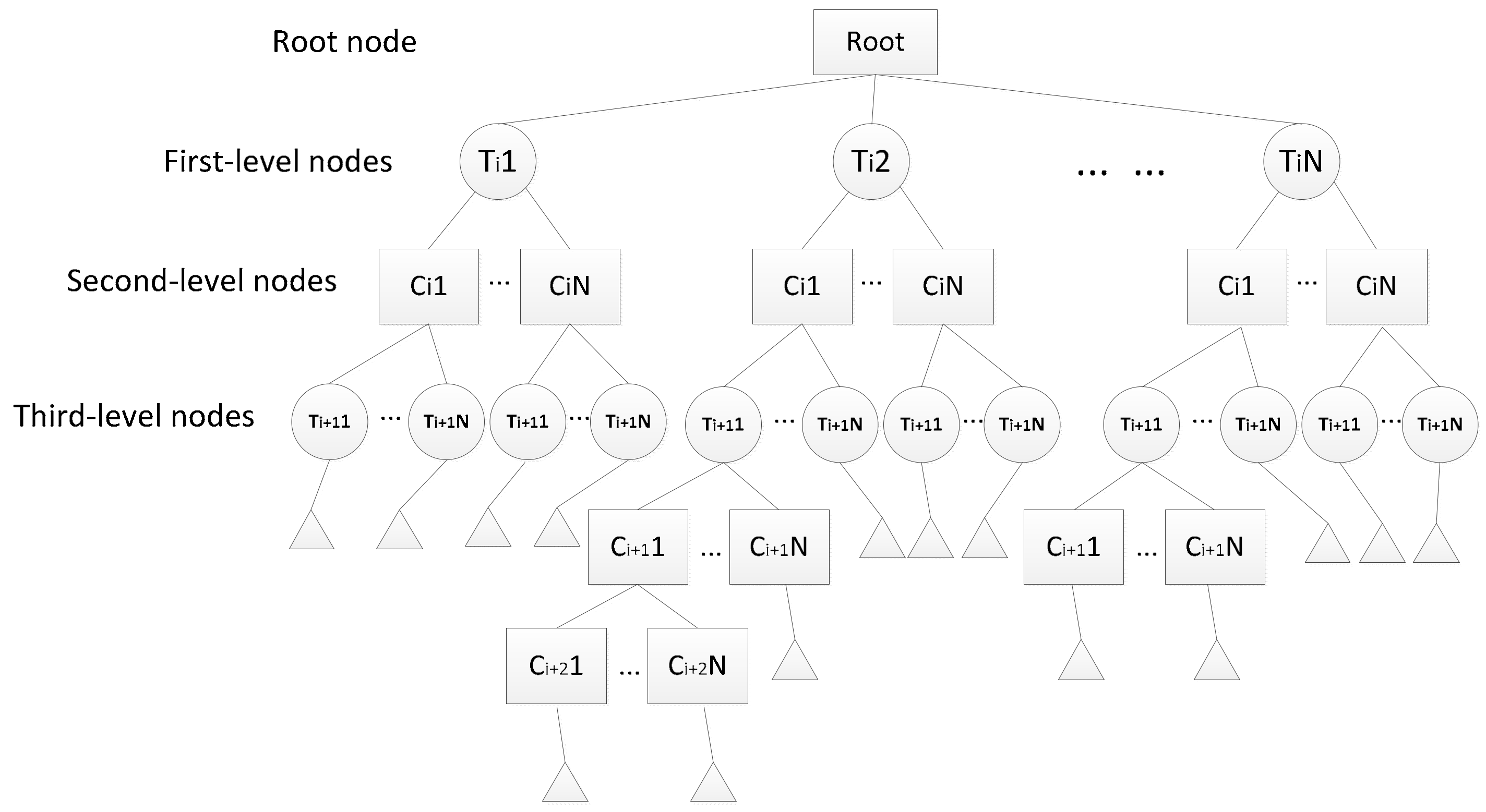
3.3.3. Multi-Level Spatio-Temporal Index Tree

Based on the method of determining the index hierarchy, this paper proposes a multi-level spatio-temporal index tree, which is suitable for spatial-temporal query and adaptive hierarchical partitioning, as shown in Figure 9. Considering the absoluteness and non-repeatability of time, the data will increase with time. To build a unified index structure for massive spatio-temporal data, the time dimension is more suitable for the initial division basis than the space dimension. Hence, the first-level node is a time information node with larger granularity, corresponding to the time information coding in the partition key of the Row Key, represented as T_i; the second-level node is the cell level, corresponding to the spatial information coding in the partition key, represented as C_i; and the third-level node is also a time information node with smaller granularity and corresponds to the time information coding of the sort key, represented as T_i+1. These three levels are initial hierarchies, and other levels can be adaptively divided according to the spatial and temporal distribution characteristics of the data, corresponding to the spatial information coding in the sort key, represented as C_i+1,2,….

The index tree can be adjusted flexibly according to the data context. For the data that pays more attention to spatial information, this index tree can be converted to the one in which spatial dimension is taken as the main partition by setting the time information in the first-level as a single node.

The specific steps of the MLS3 indexing algorithm based on the multi-level spatio-temporal index tree are as follows.

Step 1

Determine the time granularity T_partition(g_i) used in the partition key and construct a first-level node, as shown by T_i in Figure 9.

Step 2

According to the idea of the S2 index, define the MBR of a certain spatial range as Rect and convert its four-corner latitude and longitude coordinates (Rect_k, k = 0, 1, 2, 3) into three-dimensional coordinates. The rectangular spatial range Rect is used as the root node of index tree.

Step 3

Divide the projected four-corner coordinate into different levels n, n ∈ [0, 30]. The value range of n is determined by the spatial range of cell in each level of S2 index, as shown in

Table 2. Spatial range of cell in each level of S2 index.

Level	Min Area	Max Area	Avg. Area
0	85,011,012.00 km2	85,011,012.00 km2	85,011,012.00 km2
1	21,252,753.00 km2	21,252,753.00 km2	21,252,753.00 km2
2	5,313,188.25 km2	5,313,188.25 km2	5,313,188.25 km2
…	…	…	…
29	1.77 cm2	3.71 cm2	2.95 cm2
30	0.43 cm2	0.93 cm2	0.74 cm2

[15], the minimum area that a single grid can describe in level 30 is 0.43 cm², which means every cm² can be represented using a 64-bit integer and this is fine enough for the common spatial data management scenarios [30,31]. Starting from level n = 0, the current Region(face, i_k, j_k) can be covered by m cells, if m > threshold (N₁), the current level is the desired level and it is used as the second-level node C_i.

Step 4

Construct the time granularity information in the sort key, i.e., T_sort(g_i), as a third-level node, as shown by T_i+1 in Figure 9.

Step 5

Sample the elements in the entire layer and count the number of elements in the cell. If the number is larger than the threshold Split_thresh, C_i is split further. The threshold Split_thresh is an empirical value, which we obtained through a large number of actual data experiments. In this paper, we set it as 30% of the total elements. Different from the quadtree split of four cells, the only sub-cell that is split is that covering the element as sub-tree nodes of the third-level node T_i+1, and the maximum number of sub-cells is 4. Step 5 is then repeated for the sub-cells until the number of elements is less than the threshold or the depth of the sub-tree reaches the depth threshold Height_thresh(thresh). The level is set as sublevel, and the splitting is stopped.

Step 6

By mapping the m-th quadtree unit cells identified by (face, i_k, j_k) to the Hilbert curve of sublevel, the corresponding cell ID set S_cell is calculated. S_cell can uniquely represent the query area, where each cell ID of S_cell represents a sub-area of a query. All the cell IDs in S_cell are used as the level nodes and serve as the encoding of the spatial information in the sort key.

Step 7

According to the first- and second-level nodes, the Murmur Hash function is substituted to calculate the corresponding partition location, and the locations of the third-level node and its sub-tree leaf node are determined according to the cell ID.

As shown in Figure 9, MLS3 is a global index structure, which is more suitable to the P2P network. The index is stored as an array in the metadata of the NoSQL database, which includes the node information and the relationship between each node.

3.3.4. Dynamic Update and Maintenance of Multi-Level Sphere 3 (MLS3)

The update and maintenance of MLS3 can be divided into three basic operations: insert, delete and split of nodes. The detail algorithms are as follows:

• Insert operation: for the new added data, the cell ID will be calculated first. If the time information does not belong to the current index tree, a new first-level node and a new index tree branch will be added. Otherwise, determine the first-level node of the new data according to the cell ID, and then traverse the sub-tree layer by layer from the first-level node to the leaf node to find whether the node containing the new data exists. If not, insert the new data as a new leaf node; if it exists, the node is no longer need to insert [4,6].
• Delete operation: if the deleted node is a leaf node, it can be deleted directly; otherwise it cannot be deleted. If the deleted leaf node has the same level node, the delete operation is terminated and if there are no other nodes in the same level of the leaf node, the parent node is deleted. Traverse the sub-tree in turn and repeat the above step [4,6].
• Split operation: if the number of elements in a cell is larger than the threshold Split_thresh, this cell is split further. Different from the quadtree split of four cells, only the sub-cell that covering the element as sub-tree nodes of the third-level node T_i+1 is split, and the maximum number of sub-cells is 4. The split operation is repeated for the sub-cells until the number of elements is less than the threshold or the depth of sub-tree reaches the depth threshold Height_thresh(thresh).

In addition, the update and maintenance of the index algorithm constructed in this paper does not include merge operation. MLS3 is present as a way of spatio-temporal information encoding in Row Key, and the Row Key is hashed to achieve distributed storage of spatio-temporal data in the P2P network, as shown in Figure 1. Merge operation will change the Row Key value that has been assigned to the storage node, which will result in the data retrieval error. Hence, if a certain number of delete operations are performed, and only one leaf node is left in a level, we will not merge it into its parent node to ensure the stability of index.

This index tree propose in this paper is stored in the corresponding metadata as an index strategy and serves as a foundation for dividing the query range into several cell areas during querying. The traversal query time complexity is O(n), where n is the number of cells in the query range.

4. Results and Discussion

4.1. Experimental Data and Environment

To verify the validity and rationality of the MLS3 index proposed in this paper, comparative analysis with the XZ3 index was implemented with the same dataset and test environment. The P2P structure was used to build a Cassandra cluster. with a total of five database nodes, and the redundant backup factor was 2. The performance of a single node was based on an IBM X3850 Server, with 16G of memory, and a central processing unit (CPU) with 16 cores × 2.294 GHz.

The test dataset (TDrive dataset) was obtained from the global positioning system (GPS) trajectory (point element) data of 10,357 taxis in Beijing from 2 February to 8 February 2008, provided by Microsoft Research Asia [32,33]. The dataset contained 15 million pieces of data with a mileage of about 9 million kilometers. Data from November 2017 to March 2018 (5 months) in Beijing provided by Open Street Map (OSM) were also considered, including 227,258 buildings (polygon elements) and 309,314 roads (line elements) (OSM dataset) [34,35].

To test the query effect in a concurrent access environment, 200 spatio-temporal query windows for the two aforementioned datasets were generated randomly, as shown in Figure 10.

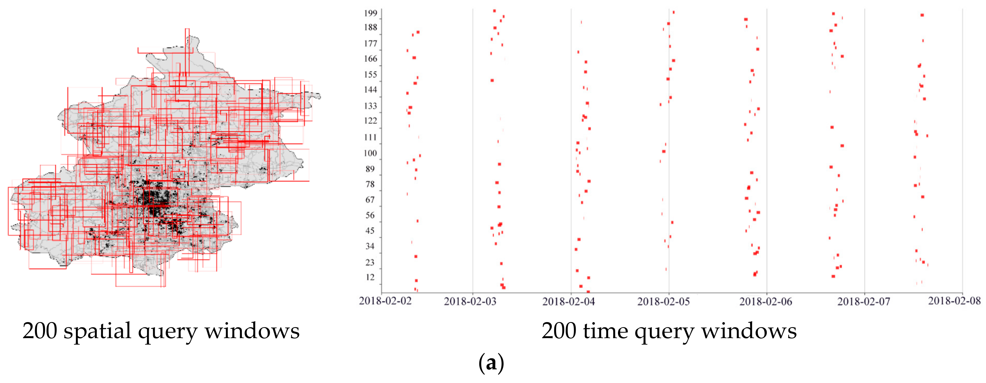
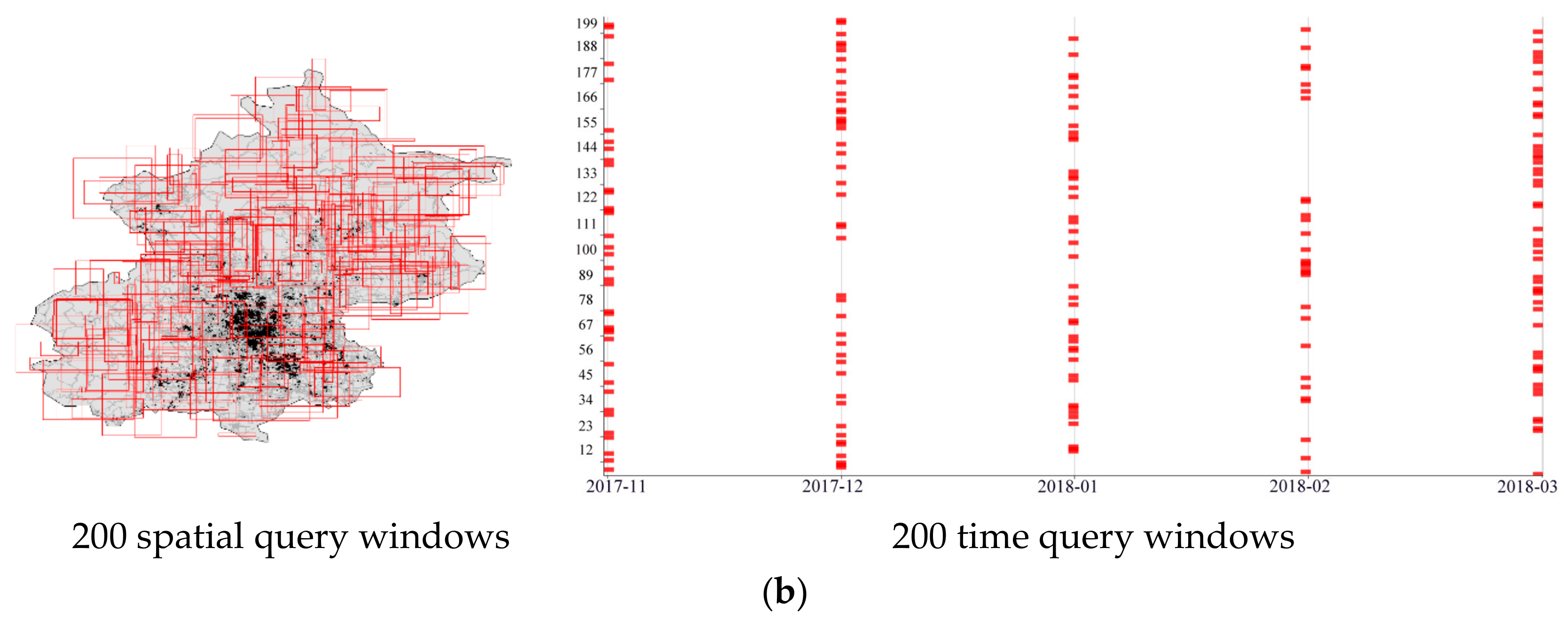
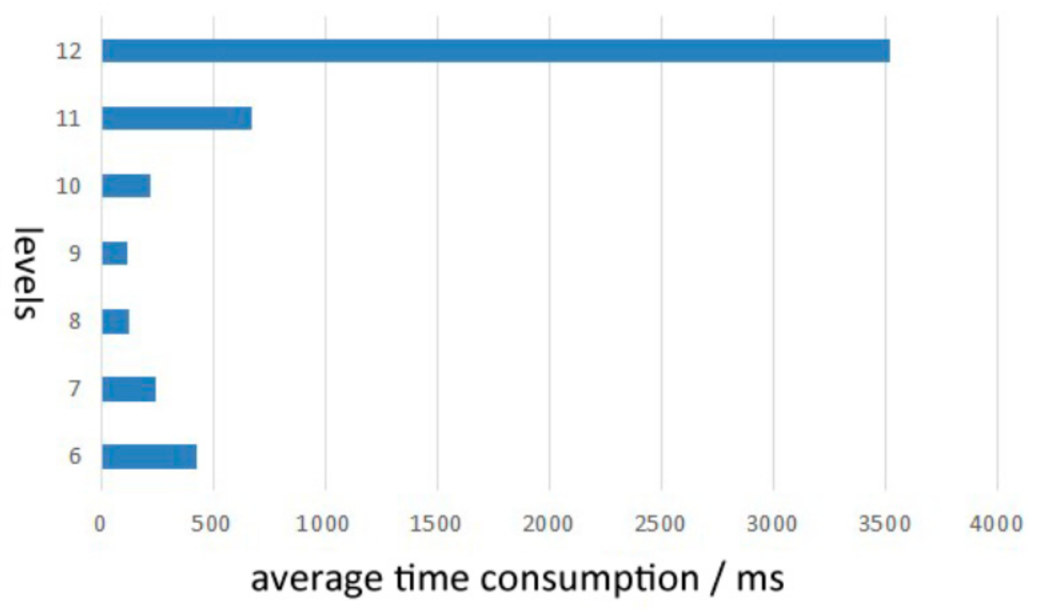
4.2. Rationality Verification of Hierarchy Determination

To verify the rationality of the division algorithm proposed in this study, the TDrive dataset was selected for testing. More than 15 million GPS data were randomly sampled, the sampling rate was 20%, and the cell splitting threshold Split_thresh was set to 30% of the sample. Setting the tree depth threshold to 2, the optimal initial level of the data set was determined to be level 9, which was calculated by using the MLS3 algorithm, the multi-level division range included levels 9–11. The time used to determine the optimal level is 1601 ms.

To verify that level 9 was the optimal level, we selected seven different levels, levels 6, 7, 8, 9, 10, 11, and 12, setting them as the initial level in the same data set. The level yielding the lowest average time consumption of 200 spatio-temporal queries among these levels was identified as the optimal level. The experimental results are shown in Figure 11. It is evident that with increasing level, the average time consumption of the query first decreases and then increases. The average time consumption gradually decreases from level 6 to level 9, and the minimum is reached at level 9. This is because with the increase of the level, the query scope was gradually refined, the partitioned ineffective query cell was gradually reduced, and the amount of query data was reduced. However, from level 9 to level 12, the average time consumption gradually increases, reaching 3520 ms at level 12. A large number of queries led to an increase of disk input and output (IO) and communication costs, resulting in a significant increase in query time. Therefore, it can be concluded that the MLS3 indexing method is effective and is well balanced between reducing the number of ineffective query cells and increasing the number of effective query cells.

The reference value of the number threshold of the cells in the first level is calculated as follows: for the experiment environment in this paper, we used a CPU with 16 cores, which can offer 16 concurrent threads parallel computing capability. In general, the acceptable time of a single query response in the database is less than 5 s [36,37]. For common spatio-temporal queries, as we can see in the experiment in this paper (

Table 3. Comparison of average query time-consuming under different number of tasks concurrency.

Number of Concurrent Tasks			1	5	10	15	20	25	30	35	40
Average time consumption (ms)	TDrive Taxi (Point)	XZ3	1623	1628	2165	2285	2317	2401	2245	2606	2373
		MLS3	526	625	642	788	676	981	1011	1461	1216
	OSM Roads (line)	XZ3	2213	1931	2632	4177	4948	5106	5422	4036	5729
		MLS3	520	626	694	836	872	1953	2861	3365	3958
	OSM Buildings (polygon)	XZ3	2215	1869	2365	3239	3662	4477	4270	4417	4430
		MLS3	374	446	459	521	523	622	595	993	969

), the query time of a single thread is about 400–500 ms. Hence, the upper and lower limits of query times in 5 s are 5 s × 1000/400 ms × 16 ≈ 200 and 5 s × 1000/500 ms × 16 ≈ 160, which are considered as the optimal level cell number threshold in this paper. In addition, considering that not every spatio-temporal query needs to traverse all cells, so the threshold value is set to 200 in this paper, and this value is also verified in the aforementioned TDrive dataset of Beijing, the experimental results show that this value is available. For new input data, we can quickly determine the optimal index level according to the data spatial range and the empirical value of 200. Assuming that the spatial region area is S, the corresponding MBR area is S_MBR, the average cell area in each level is AS_level(i), then calculate the minimum value of the differences between $S_{MBR}/200$ and ${AS}_{level\left(i\right)}$ as following formula (6). The level corresponding to the minimum value is taken as the most suitable level for the new data.

$$min(\frac{S_{MBR}}{200}-{AS}_{level\left(1\right)},\frac{S_{MBR}}{200}-{AS}_{level\left(2\right)},\dots ,\frac{S_{MBR}}{200}-{AS}_{level\left(i\right)},\dots ,\frac{S_{MBR}}{200}-{AS}_{level\left(30\right)})$$

(6)

According to this algorithm, we have ascertained that the most suitable level for the national layer (such as in the Chinese national range) is 4–5, for the provincial layer (such as in the Shandong Province range) is 7–8, and for the city layer (such as in the Beijing area) is 9–10. The level ranges have been verified in the projects of spatio-temporal information cloud platform construction in Smart Linyi and Smart Zibo, which are two cities in Shandong province of China.

4.3. Comparison of Index Performance

The XZ3 spatio-temporal index algorithm (Source code: https://github.com/locationtech/geomesa/releases/tag/geomesa_2.11-2.3.1), which was published in 2019, is selected to compare with the proposed MLS3 algorithm using the same data set and environment for query performance testing. The latest upadate of XZ3 algorithm is Version 2.3.1, and in this version GeoMesa gives the default parameter values which show the optimal performance of the algorithm to developers. Hence, these default parameter values will be used in this paper. The performance of our index is tested from three aspects: index query efficiency, construction efficiency and space consumption ratio.

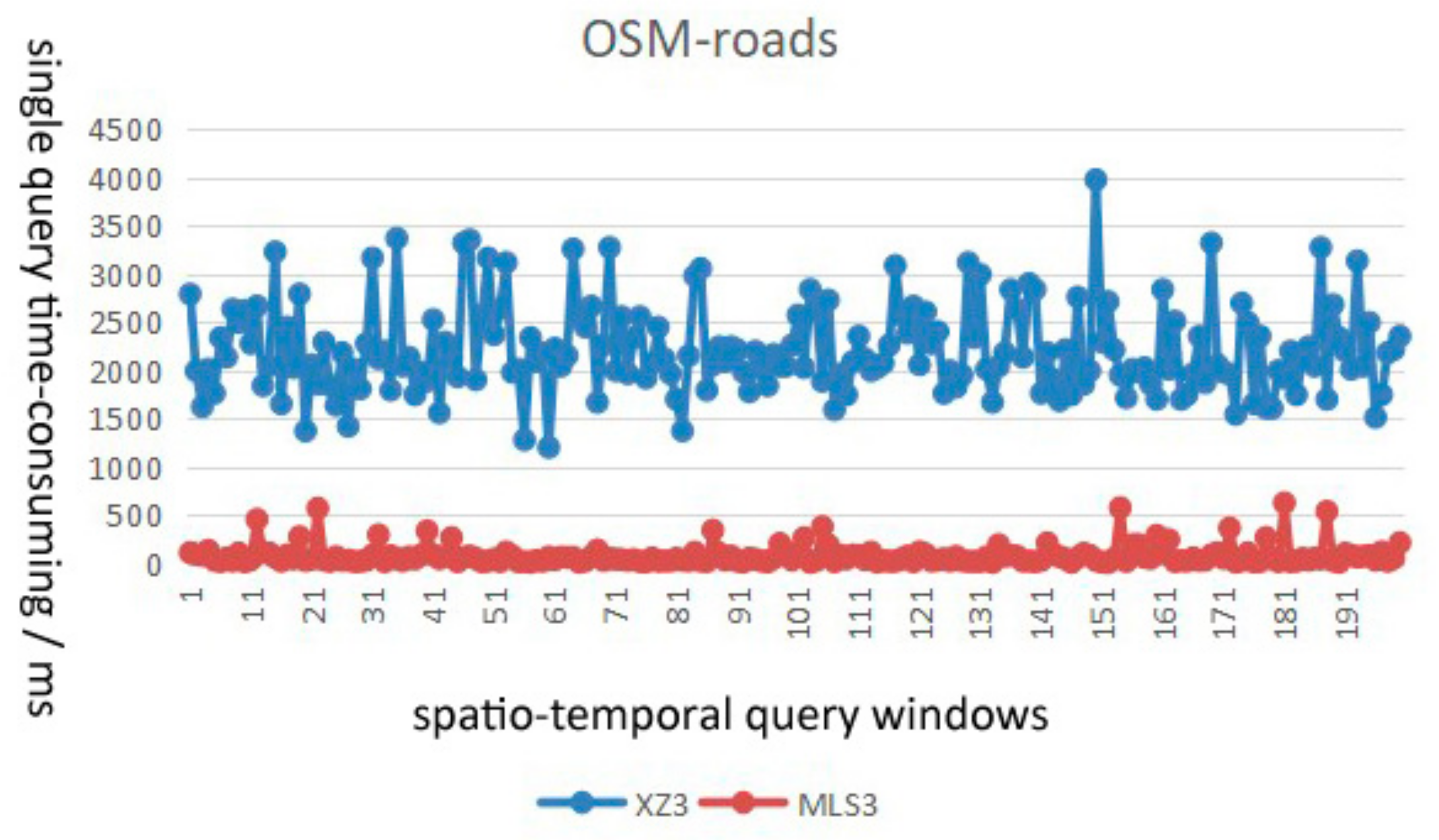
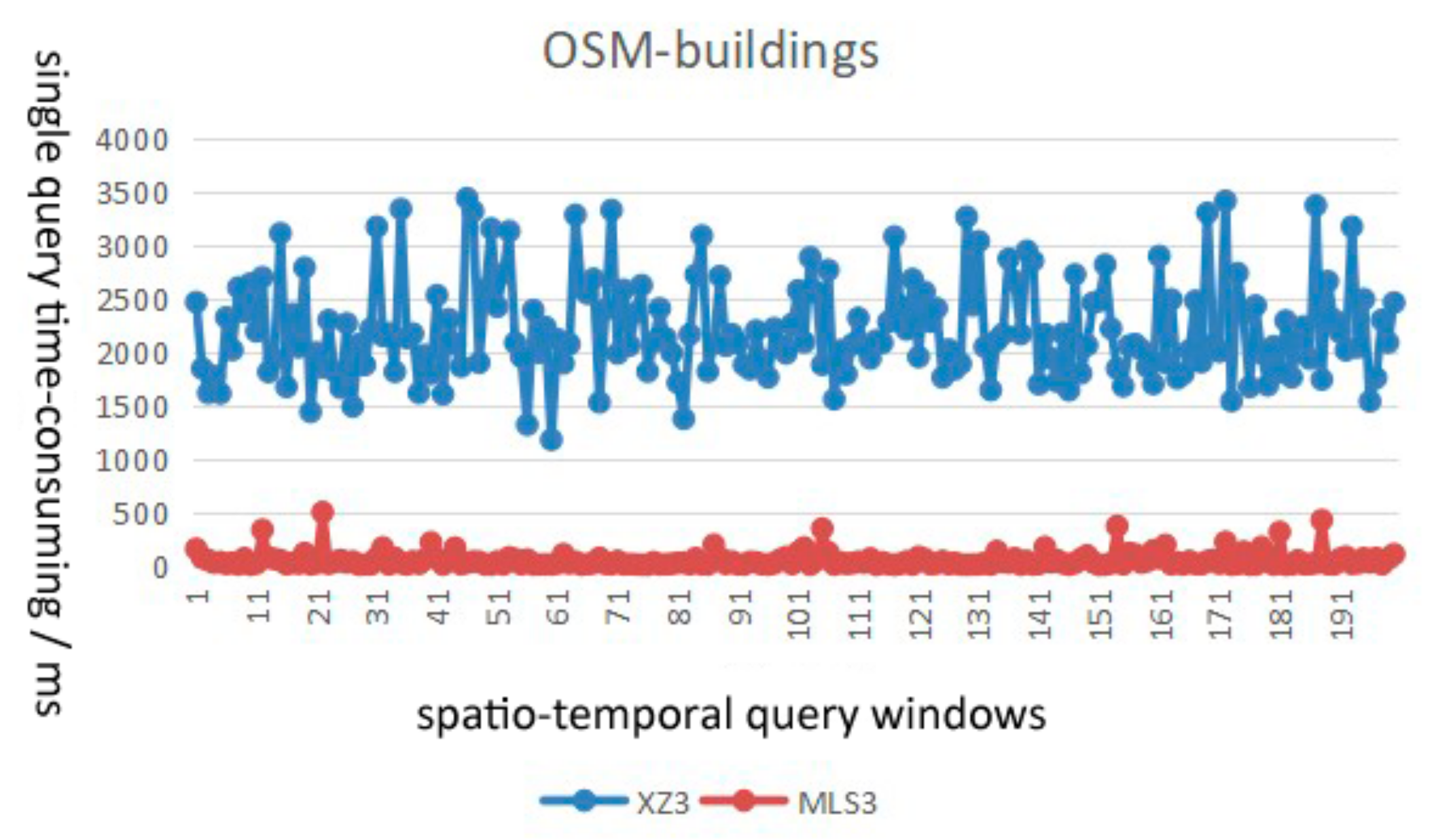
4.3.1. Index Query Efficiency

Since the XZ3 algorithm defaults to a single thread with page size 1, which is provided by GeoMesa, we first compared the performances of the two algorithms under the default parameter settings. The TDrive and OSM datasets were used as the experimental data. Multiple sets of concurrent query access were assigned granularity of 1, 5, 10, 15, 20, 25, 30, 35, and 40.

As shown in Table 3, with an increase in concurrent query access tasks, the average query time consumptions of the MLS3 and XZ3 indexing algorithms both increase, but the MLS3 algorithm requires less time than the XZ3 algorithm. As shown in Table 3, for the query of the spatio-temporal GPS trajectory points in the TDrive dataset, the time consumption of the XZ3 algorithm is 1.7–3.4 times greater than that of the MLS3 algorithm. For non-point layer elements such as lines and polygons in particular, the MLS3 algorithm exhibits more significant improvement. The MLS3 algorithm greatly alleviated the pressure of complex spatio-temporal query operations under high concurrency conditions, and its time consumption was about 1/7–1/2 that of the XZ3 algorithm.

In addition, we optimized the parameters of our method and compared it with the XZ3 method. The MLS3 approach used five threads, with a page size of 1024, while the XZ3 algorithm employed the default parameters. The experimental results are shown in Figure 12, Figure 13 and Figure 14. It can be seen that for three types of data (points, lines, and polygons), the query time consumption with the XZ3 algorithm fluctuates considerably, which is due not only to the amount of data used in the query process, but also to the type of SFC utilized in the indexing algorithm. The XZ3 algorithm uses the Z-order curve, which has the problem that the spatial relationships of adjacent data may hop.

In this study, the Hilbert curve was used in the MLS3 algorithm to ensure that the spatial adjacent elements were encoded adjacently. For the three types of data, the time consumption of the MLS3 algorithm fluctuates within 2000 ms (Figure 12), 630 ms (Figure 13) and 500 ms (Figure 14). Overall, the MLS3 algorithm exhibits greatly improved performance under the condition of multi-threading and appropriate page size, the query efficiency is improved by 4–7 times, and the query time consumption is stable, which is better suited for practical scenarios.

4.3.2. Construction Efficiency and Space Consumption Ratio

Taking the generation time of experimental data index as the construction efficiency and the ratio of index data volume to corresponding vector data volume as the space consumption ratio, the calculation results of the two index methods in each indicator are shown in

Table 4. Comparison of index space consumption rate and construction efficiency.

Indicator	Index Method	TDrive Taxi (Point)	OSM Roads (Line)	OSM Buildings (Polygon)
Space consumption ratio	XZ3	31.14%	7.37%	10.68%
	MLS3	38.63%	8.91%	13.70%
Construction efficiency (s)	XZ3	63	2	2
	MLS3	147	23	19

. It can be found that for point, line and polygon elements, the spatial consumption ratio of our method is slightly higher than that of XZ3 index, which increases by 7.49%, 1.54% and 3.02%, respectively. However, compared with the total storage space of 120G, the data volume of the two indexing methods accounts for about 0.5%, which indicated the space consumption rate is acceptable in the existing hardware storage environment. In addition, in terms of index construction efficiency, the construction time of this method is higher than XZ3, and the increased time is positively correlated with the number of data elements. This is because XZ3 only calculates the Row Key value, while MLS3 needs to construct a multi-level index tree and determine the optimal index level. However, it is worth pointing out that the construction process does not take more than 1/10 of the total time of data import.

5. Conclusions

To address the issues existing in traditional spatio-temporal indexing, an adaptive hierarchical spatio-temporal index algorithm was developed in this study. This algorithm can not only describe vector data reasonably, but also improves the efficiency of spatio-temporal retrieval and avoids storage hotspots in P2P networks. Compared with the XZ3 spatio-temporal index, the MLS3 index proposed in this paper has three main advantages: (1) in the time dimension, the hierarchical index structure with different granularity is added to improve query efficiency; (2) in the space dimension, the Z-order curve is replaced by a Hilbert curve to solve the querying hopping problem; (3) the temporal and spatial index are integrated into a spatio-temporal index, which does not simply sequence a spatial index or a time index, to support joint spatio-temporal query.

Based on validation with a large number of actual data, the main contributions of this study can be summarized as follows:

(1)

To determine the optimal hierarchy, the spatial distribution and density of the entire layer of elements were considered. The most suitable level for the national layer is 4–5, for the provincial layer 7–8, and for the city layer 9–10.

(2)

In terms of query efficiency, the average time consumption of the proposed MLS3 algorithm is about 1/7–1/2 of that of the XZ3 algorithm with the same parameters, and the query efficiency of the MLS3 index can be improved by 4–7 times after parameter optimization.

(3)

In terms of query stability, the MLS3 index with a Hilbert filling curve can better describe the continuity of spatio-temporal data than the XZ3 index with a Z-order filling curve. The MLS3 index shows more stable query performance and is more suitable for distributed storage management of massive multi-scale data.

(4)

In terms of space consumption ratio, our method sacrifices part of the storage space for an efficient query; however, the storage space of the index accounts for about 0.5% of total hardware storage space, which is acceptable for the spatio-temporal big data storage and management.

In future work, the construction efficiency and space consumption ratio will be optimized and we will extend the MLS3 index algorithm to the distributed NoSQL databases of client servers. In addition, the index algorithm proposed in this paper is mainly used to locate the storage nodes on P2P networks quickly and efficiently retrieve the data on the nodes, but the data spread between each node is not discussed. Addressing this issue is beyond the scope of this research, but it is a promising direction for further exploration.

References

1. Cornelli, F.; Damiani, E.; Di Vimercati, S.D.C.; Paraboschi, S.; Samarati, P. Choosing reputable servents in a P2P network. In Proceedings of the 11th International Conference on World Wide Web, Honolulu, HI, USA, 7–11 May 2002; pp. 376–386. [Google Scholar]
2. Kostakis, V.; Bauwens, M.; Niaros, V. Urban Reconfiguration after the emergence of peer-to-peer infrastructure: Four future scenarios with an impact on smart cities. In Smart Cities as Democratic Ecologies; Palgrave Macmillan: London, UK, 2015; pp. 116–124. [Google Scholar]
3. Santos, J.; Wauters, T.; Volckaert, B.; De Turck, F. Fog computing: Enabling the management and orchestration of smart city applications in 5g networks. Entropy 2018, 20, 4. [Google Scholar] [CrossRef]
4. Alarabi, L.; Mokbel, M.F.; Musleh, M. St-hadoop: A mapreduce framework for spatio-temporal data. GeoInformatica 2018, 22, 785–813. [Google Scholar] [CrossRef]
5. Shen, D.; Yu, G.; Wang, X.; Nie, T.; Kou, Y. Survey on NoSQL for management of big data. J. Softw. 2013, 24, 1786–1803. (In Chinese) [Google Scholar] [CrossRef]
6. John, A.; Sugumaran, M.; Rajesh, R.S. Indexing and query processing techniques in spatio-temporal data. ICTACT J. Soft Comput. 2016, 6. [Google Scholar] [CrossRef]
7. Aguilera, M.K.; Golab, W.; Shah, M.A. A practical scalable distributed B-tree. In Proceedings of the VLDB. Morgan Kaufmann, Auckland, New Zealand, 24–30 August 2008. [Google Scholar]
8. Cary, A.; Sun, Z.; Hristidis, V.; Rishe, N. Experiences on processing spatial data with MapReduce. In Proceedings of the Scientific and Statistical Database Management, International Conference (SSDBM 2009), New Orleans, LA, USA, 2–4 June 2009; pp. 302–319. [Google Scholar]
9. Mouza, C.; Litwin, W.; Rigaux, P. Large-scale indexing of spatial data in distributed repositories: The SD-Rtree. VLDB J. 2009, 18, 933–958. [Google Scholar] [CrossRef]
10. Wu, S.; Jiang, D.W.; Ooi, B.C.; Wu, K.L. Efficient B-tree based indexing for cloud data processing. Proc. VLDB Endow. 2010, 3, 1207–1218. [Google Scholar] [CrossRef]
11. Eldawy, A.; Mokbel, M.F. Spatialhadoop: A mapreduce framework for spatial data. In Proceedings of the 2015 IEEE 31st International Conference on Data Engineering, Seoul, Korea, 13–17 April 2015; pp. 1352–1363. [Google Scholar]
12. Yu, J.; Zhang, Z.; Sarwat, M. Spatial data management in apache spark: The geospark perspective and beyond. Geoinformatica 2019, 23, 37–78. [Google Scholar] [CrossRef]
13. Fox, A.; Eichelberger, C.; Hughes, J.; Lyon, S. Spatio-temporal indexing in non-relational distributed databases. In Proceedings of the IEEE International Conference on Big Data, Silicon Valley, CA, USA, 6–9 October 2013; pp. 291–299. [Google Scholar]
14. Le, H.V.; Atsuhiro, T. An efficient distributed index for geospatial databases. In Database and Expert Systems Applications; Springer: Cham, Switzerland, 2015; pp. 28–42. [Google Scholar]
15. Google Corporation. S2 Geometry Library. 2015. Available online: http://s2geometry.io/ (accessed on 6 April 2019).
16. Procopiuc, O. Geometry on the Sphere: Google’s S2 Library. 2011. Available online: https://docs.google.com/presentation/d/1Hl4KapfAENAOf4gv-pSngKwvS_jwNVHRPZTTDzXXn6Q/view#slide=id.i22 (accessed on 7 April 2019).
17. Hughes, J.N.; Annex, A.; Eichelberger, C.N.; Fox, A.; Hulbert, A.; Ronquest, M. GeoMesa: A Distributed Architecture for Spatio-Temporal Fusion. In Geospatial Informatics, Fusion, and Motion Video Analytics V; International Society for Optics and Photonics: Baltimore, MD, USA, 20 April 2015. [Google Scholar]
18. Böxhm, C.; Klump, G.; Kriegel, H.P. XZ-Ordering: A space-filling curve for objects with spatial extension. In International Symposium on Advances in Spatial Databases; Springer: Berlin, Germany, 1999. [Google Scholar]
19. Zhang, R.; Qi, J.; Stradling, M.; Huang, J. Towards a painless index for spatial objects. ACM Trans. Database Syst. 2014, 39, 19. [Google Scholar] [CrossRef]
20. Fecher, R.; Whitby, M.A. Optimizing Spatiotemporal Analysis Using Multidimensional Indexing with GeoWave. Free Open Source Softw. Geospat. Conf. Proc. 2017, 17, 12. [Google Scholar]
21. Eldawy, A.; Alarabi, L.; Mokbel, M.F. Spatial partitioning techniques in SpatialHadoop. Proc. VLDB Endow. 2015, 8, 1602–1605. [Google Scholar] [CrossRef]
22. Eldawy, A. SpatialHadoop: Towards flexible and scalable spatial processing using MapReduce. In Proceedings of the Sigmod PhD Symposium, Snowbird, UT, USA, 22 June 2014; pp. 46–50. [Google Scholar]
23. Whitman, R.T.; Park, M.B.; Ambrose, S.M.; Hoel, E.G. Spatial indexing and analytics on Hadoop. In Proceedings of the 22nd ACM SIGSPATIAL International Conference on Advances in Geographic Information Systems, Dallas, TX, USA, 4–7 November 2014; pp. 73–82. [Google Scholar]
24. Lakshman, A.; Malik, P. Cassandra: A structured storage system on a P2P network. In Proceedings of the ACM Symposium on Parallelism in Algorithms and Architectures, Calgary, AB, Canada, 10–12 August 2009; p. 47. [Google Scholar]
25. Lakshman, A.; Malik, P. Cassandra: A decentralized structured storage system. ACM SIGOPS Oper. Syst. Rev. 2010, 44, 35–40. [Google Scholar] [CrossRef]
26. Brahim, M.B.; Drira, W.; Filali, F.; Hamdi, N. Spatial data extension for Cassandra NoSQL database. J. Big Data 2016, 3, 1–16. [Google Scholar] [CrossRef]
27. Chebotko, A.; Kashlev, A.; Lu, S. A big data modeling methodology for Apache Cassandra. In Proceedings of the IEEE International Congress on Big Data, New York, NY, USA, 27 June–2 July 2015; pp. 238–245. [Google Scholar]
28. Belussi, A.; Migliorini, S.; Eldawy, A. Detecting skewness of big spatial data in SpatialHadoop. In Proceedings of the 26th ACM SIGSPATIAL International Conference on Advances in Geographic Information Systems, Seattle, WA, USA, 6–9 November 2018; pp. 432–435. [Google Scholar]
29. González, R.; Munoz, A.; Hernández, J.A.; Cuevas, R. On the tweet arrival process at Twitter: Analysis and applications. Trans. Emerg. Telecommun. Technol. 2014, 25, 273–282. [Google Scholar] [CrossRef]
30. Shaw, B.; Shea, J.; Sinha, S.; Hogue, A. Learning to rank for spatiotemporal search. In Proceedings of the Sixth ACM International Conference on Web Search and Data Mining, Rome, Italy, 4–8 February 2013; pp. 717–726. [Google Scholar]
31. Weyand, T.; Kostrikov, I.; Philbin, J. PlaNet—Photo Geolocation with Convolutional Neural Networks. In European Conference on Computer Vision; Leibe, B., Matas, J., Sebe, N., Welling, M., Eds.; Springer: Cham, Switzerland, 2016. [Google Scholar]
32. Yuan, J.; Zheng, Y.; Zhang, C.; Xie, W.; Xie, X.; Sun, G.; Huang, Y. Tdrive: Driving directions based on taxi trajectories. In Proceedings of the 18th SIGSPATIAL International Conference on Advances in Geographic Information Systems, GIS’10, San Jose, CA, USA, 2–5 November 2010; pp. 99–108. [Google Scholar]
33. Yuan, J.; Zheng, Y.; Xie, X.; Sun, G. Driving with knowledge from the physical world. In Proceedings of the 17th ACM SIGKDD International Conference on Knowledge Discovery and Data Mining, KDD’11, San Diego, CA, USA, 21–24 August 2011; pp. 316–324. [Google Scholar]
34. Curran, K.; Fisher, G.; Crumlish, J. OpenStreetMap. Int. J. Interact. Commun. Syst. Technol. 2012, 2, 69–78. [Google Scholar] [CrossRef]
35. Haklay, M.; Weber, P. OpenStreetMap: User-generated street maps. IEEE Pervasive Comput. 2008, 7, 12–18. [Google Scholar] [CrossRef]
36. Shao, J.; Liu, X.; Li, Y.; Liu, J. Database performance optimization for SQL Server based on hierarchical queuing network model. Int. J. Database Theory Appl. 2015, 8, 187–196. [Google Scholar] [CrossRef]
37. Cao, Y.; Ritz, C.; Raad, R. How much longer to go? The influence of waiting time and progress indicators on quality of experience for mobile visual search applied to print media. In Proceedings of the 2013 Fifth International Workshop on Quality of Multimedia Experience (QoMEX), Klagenfurt am Wo¿rthersee, Austria, 3–5 July 2013; pp. 112–117. [Google Scholar]
Figure 1. Spatio-temporal index framework.
Ijgi 08 00512 g001
Figure 2. Time information part in Row Key (‘……’ refers to other parts in Row Key).
Ijgi 08 00512 g002
Figure 3. Spatial information coding.
Ijgi 08 00512 g003
Figure 4. Spatial information part in Row Key (‘……’ refers to other parts in Row Key).
Ijgi 08 00512 g004
Figure 5. Feature identification (FID) part in Row Key.
Ijgi 08 00512 g005
Figure 6. Design of Row Key.
Ijgi 08 00512 g006
Figure 7. Row Key of point element.
Ijgi 08 00512 g007
Figure 8. Row Key of line element.
Ijgi 08 00512 g008
Figure 9. Multi-level spatio-temporal index tree (T is related to time and C is related to space).
Ijgi 08 00512 g009
Figure 10. Two hundred space-time query windows distribution: (a) TDrive dataset and (b) Open Street Map (OSM) dataset.
Ijgi 08 00512 g010aIjgi 08 00512 g010b
Figure 11. Average time consumption at different levels.
Ijgi 08 00512 g011
Figure 12. Query time consumption comparison of the global positioning system (GPS) points in the TDrive dataset.
Ijgi 08 00512 g012
Figure 13. Query time consumption comparison of the road layer in the OSM dataset.
Ijgi 08 00512 g013
Figure 14. Query time consumption comparison of the building layer in the OSM dataset.
Ijgi 08 00512 g014