Simulating Uneven Urban Spatial Expansion under Various Land Protection Strategies: Case Study on Southern Jiangsu Urban Agglomeration

Abstract

Urban spatial expansion (USE) is an uneven process affected by both natural and human factors, and land use regulation policy is of significance. To indicate the potential effects of different policies at a regional scale and then improving them under the context of increasing emphasis on land protection, we take Southern Jiangsu Urban Agglomeration (SJUA) in eastern China as a case study. Based on USE simulation with a minimum cumulative resistance (MCR) model under four scenarios related with arable and ecological land protection, we analyze the spatial differentiation of newly added urban construction lands and examine the changes of urban system with fractal analysis. Results indicate the allocations of newly added urban construction land differs by scenarios as well as total expanding amounts, and larger cities tend to grow faster. The share of the four largest cities (Suzhou, Nanjing(S), Wuxi, and Changzhou) were mostly higher than 40%. Accordingly, the final area of all cities was linearly corrected with their extant sizes in 2010. However, the differentiated allocations of newly added urban lands related to both increasing expanding amounts and different scenarios caused differences in the said linear relationships and also influenced urban rank-size in different degrees. It is concluded that the MCR model is feasible for simulating regional scale urban expansion and land protection strategies do not induce dramatic changes to the basic structures of regional urban system, but they are slightly different as land protection strategies change. The spatial distribution of protected lands affect the differentiation of both the predicted expanding amount of different cities and the regional urban systems significantly. It is of importance to optimize the spatial distribution of protected lands to regulate regional scale USE patterns and also urban systems properly.

1. Introduction

Urban spatial expansion (USE) is ongoing at an unprecedented speed in our world’s developing countries and regions [1]. Urban construction lands are reported to increase by 58,000 km² or 9% from 1970 to 2000 globally [2]. The share of developing countries and regions is increasing greatly, and China is a typical case with rapid urbanization where developed land increased from 13,148 km² to 35,633 km² during the period from 1990 to 2012 [3]. Among which, urban agglomerations or megacities expand faster in both developed and developing countries [4]. Six Chinese megacities (i.e., Shenzhen, Guangzhou, Chongqing, Shanghai, Tianjin and Beijing) have all undergone extensive physical expansion from 1978 to 2018, and their annual growth rates were 11.02%, 8.07%, 5.80%, 5.37%, 4.56% and 3.46%, respectively [5]. USE and the accompanied land use changes as well as high-intensity anthropogenic activities yield complicated issues such as social conflicts, economic polarization, food deficits, and ecological security problems. Accordingly, USE has long been a main target for governmental concerns and scholarly attention [6]. Early studies mostly focused on individual cities and their processes, models, influencing factors, and effects (e.g., [7,8,9]). However, as more issues are caused (and resolved) in regions composed by a group of cities, the uneven USE has received increasing research attention in recent years [10,11].

As a geographical and socioeconomic process, USE is inherently uneven due to different development opportunities [6]. The uneven occurrence is explained by different theories and affected by various factors, which are expressed by both the different extant size and expanding speed of the cities. As for the foundational support of industries and population, urban spatial expansion is primarily driven by regional industrial development and population growth; hence their differences would bring different needs for urban space, and therefore, dissimilar urban expansion [7,12]. The theory of the urban growth machine explores how economic and population growth affects patterns of urbanization, and indicates the effects of different factors [13]. The growth poles theory points out that economic growth is not uniform over an entire region, but takes place around a specific pole (or cluster), which implies uneven growth and the formation of a growth pole over a certain region [14]. According to research in developing countries including China, uneven USE is indicated to be caused by various factors including uneven public resource allocation and land systems, unequal ecological carrying capacities, and also different processes of globalization and economic growth [15].

Up to now, related research has been carried out at the international [2,16], national [17], and regional scales [18,19]. Developing countries have been of particular concern as most USE and population growth have happened there in recent decades [20]; Asia and Africa alone are estimated to dominate the future growth of the global urban population between 2014 and 2050 [21]. Moreover, uneven USE is related with inequality of regional development and human life needs to be emphasized [22]. Regional scale USE has surpassed those at an international or national scale as per the closer relationship and stronger interactions among a group of cities. Urban agglomerations (UA; similar to “megalopolis”, “desakota”, or “city cluster” concepts) are often adopted as study cases [23]. Gottmann and McGee provided valuable information regarding the spatial pattern and structure of urban expansion at the regional scale [24,25]. The following researchers explore uneven phenomena with various methodologies and datasets [17], spatial patterns and structures [26], dynamic urban systems [27,28], and influencing factors and mechanisms [11,29]; while some have centered their research on topics about land use regulation policies [11]. Most scholars focus on historical processes and current states, while few attempt to predict or simulate future possibilities related to uneven land development. A working understanding of land use changes and induced pattern of USE is necessary to establish policies that facilitate future sustainable development.

USE simulation has theoretical and practical significance in predicting future spatial patterns and revealing possibilities under different scenarios [30,31]. Researchers have explored model designing, factor selection, parameter setting, and optimization techniques for this purpose [32,33]. Unlike simulation of an individual city, regional scale USE merits specific concern regarding the uneven pattern under different opportunities and policy orientations [17,34]. As a dynamic process of land use change driven by complex forces (including social, economic, political, and physical perspectives), anthropogenic and geographical factors may be used to build models to predict various dynamics of USE [35,36]. Scholars tend to emphasize physical geographical conditions, locations, and transportation systems while neglect other restricting factors such as the distribution of strictly protected lands. Models such as Cellular Automata (CA), Conversion of Land Use and its Effects at Small Region Extent (CLUE-S), and Minimum Cumulative Resistance (MCR) are commonly used for their simplification and operability [31,34,37,38,39,40], but have yet to be expanded to include all available factors in USE simulations. Besides, the uneven expansion of urban agglomeration significantly affects regional sustainable development through continuous land development, uneven resource allocation, and imbalanced economic development [17,26]. However, few have investigated the effects of USE, especially the uneven patterns at the regional scale. It is imperative to evaluate how cities expand unevenly under different land management scenarios so as to inform policies which facilitate regional sustainable development.

In some developing countries, UAs receive over-emphasis not only in regards to their higher development stages but also their stronger international competitiveness. The Chinese National New Urbanization Plan states that “…UAs will be the major pattern of China’s new urbanization” in coming years; China has provided both policy and economic support to promote the formation and growth of UAs [23]. Moreover, as China also aims to promote ecologically safe construction and regional sustainable development, the government has strictly protected both important ecological lands and high-quality arable lands. This provides a new challenge for carrying out USE simulation of an UA and proposing suggestions on optimizing urban structure and also promoting land protection.

In this study, China’s Southern Jiangsu Urban Agglomeration (SJUA) was chosen as a case study to address the following questions: (1) How can the geographical expansion of different cities in SJUA be simulated under the restriction of different land protection policies? (2) Will the regional urban system change as cities expand unevenly? Will the differences in various expansion scenarios be related to various land protection policies?

Figure 1 shows the outline of the procedures used in this study. We firstly conducted a literature review, and then established a brief description to the study area (SJUA) before we determined the appropriate methodology and data collection process. We then ran a multi-scenario simulation of USE and analyzed the differences of the USE process and also analyzed changes of urban systems under different scenarios. Our contributions and policy implications from the perspective of optimizing land use regulation policies and promoting regional sustainable development, alongside a summary of our major findings, are provided in the last section of this paper.

2. Study Area and Methodology

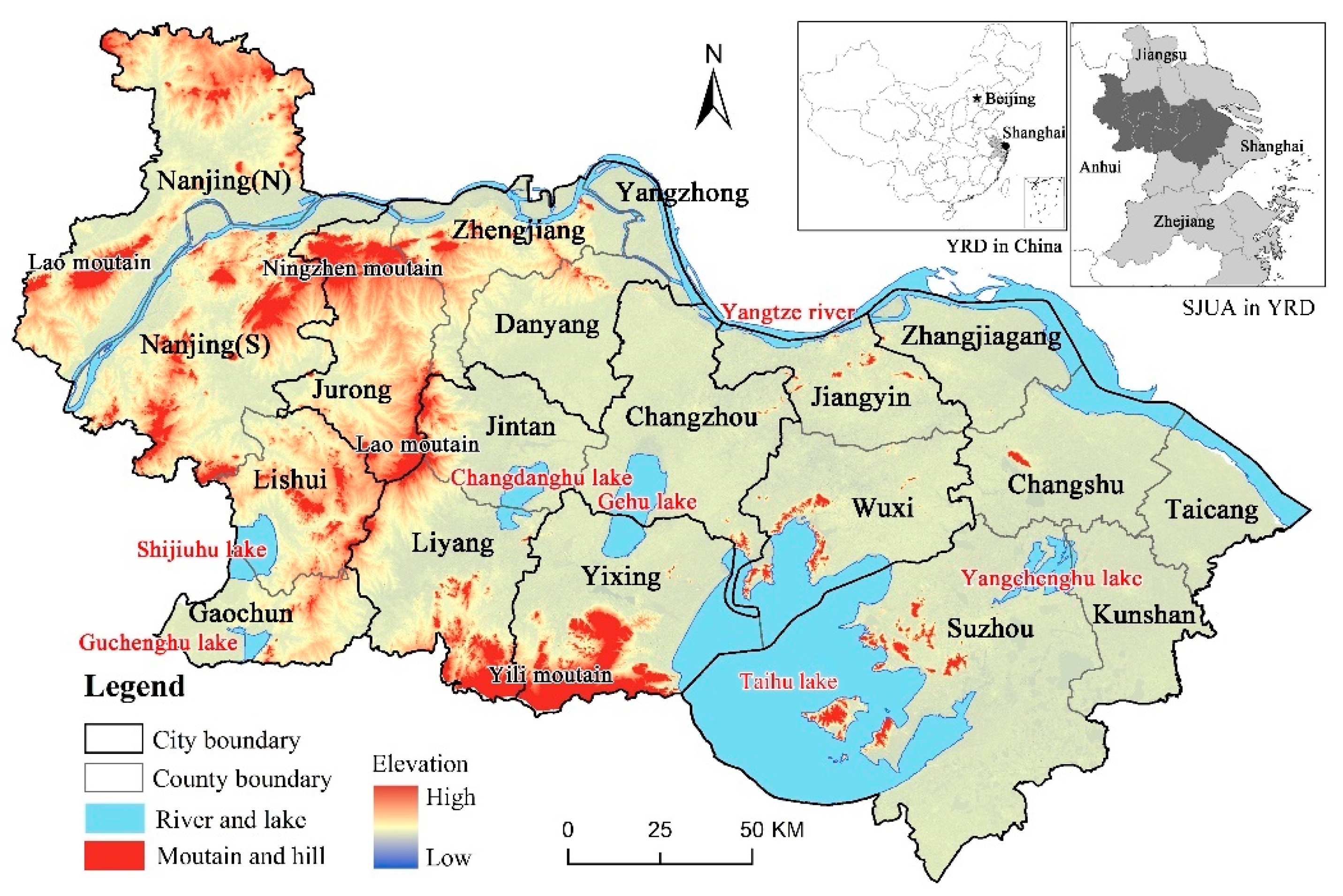
2.1. Study Area

SJUA is located at the Yangtze River Delta (YRD) and is one of the China’s most developed regions [41]. Although SJUA is part of the widely accepted YRD in eastern China, 26 administrative units in the YRD belong to four provincial-level regions which are the primary units of public administration, policy-making, and resource allocation. Different provincial jurisdictions in China lead to significant differences in land regulation policies [17], but the five prefecture-level regions of SJUA (i.e., Nanjing, Wuxi, Changzhou, Suzhou, and Zhenjiang) form an essentially homogeneous unit as they all locate at Jiangsu province. Administrative barriers do not affect different resource regulation policies greatly [6]. Therefore, SJUA is suitable as the case area.

SJUA covers a land area of 28,000 km² which is dominated by plains with an elevation consistently below 50 m, and is one of the most livable regions in China. The Yangtze River originates from the north of the region; waters including Taihu Lake, Gehu Lake, and Yangchenghu Lake account for about 21% of the whole area. Low mountains such as Yili Mountain and Ningzhen Mountain (elevation no more than 500 m) are distributed at the southern and western parts of the region. The five prefecture-level regions can be further divided into 19 cities (i.e., analytical units) based on the administrative divisions and spatial distribution of urban construction lands (Figure 2;

Table 1. Administrative divisions and cities in SJUA, 2015.

Prefecture-Level Region	Land Area (sq. km)	GDP (Billion RMB)	Population (Million Person)	City
Nanjing city	6587	972.08	8.22	Nanjing (Northern, N), Nanjing (Southern, S), Lishui, Gaochun
Wuxi city	4627	851.83	6.50	Wuxi, Jiangyin, Yixing
Changzhou city	4372	527.32	4.70	Changzhou, Jintan, Liyang
Suzhou city	8657	1450.41	10.60	Suzhou, Kunshan, Changshu, Zhangjiagang, Taicang
Zhenjiang city	3840	350.25	3.17	Zhenjiang, Yangzhong, Danyang, Jurong

Data source: Jiangsu Statistical Yearbook (2016).

).

Economic development and population agglomeration lead to an increase in construction projects. Land use data indicated that urban construction land was 3974 km² in 2010—about 2.7 times than that in 2000; while cultivated land decreased by 3131 km² and was mostly replaced by construction lands. Urban construction lands expanded with different spatial characteristics and city propers grew faster than other urban areas [27,29]. In the course of securing a sustainable and balanced urban agglomeration, SJUA needs to ensure effective regional development while optimizing the urban system structure [42]. As the most important input for USE, the allocation of newly added construction land is certain to affect the uneven expansion of different cities greatly. Up to now, various policies have been made to regulate land development and promote land protection, which might affect the allocation of newly added construction land and then the uneven pattern of regional USE. It is necessary to evaluate the effect of different land regulation policies to optimize them.

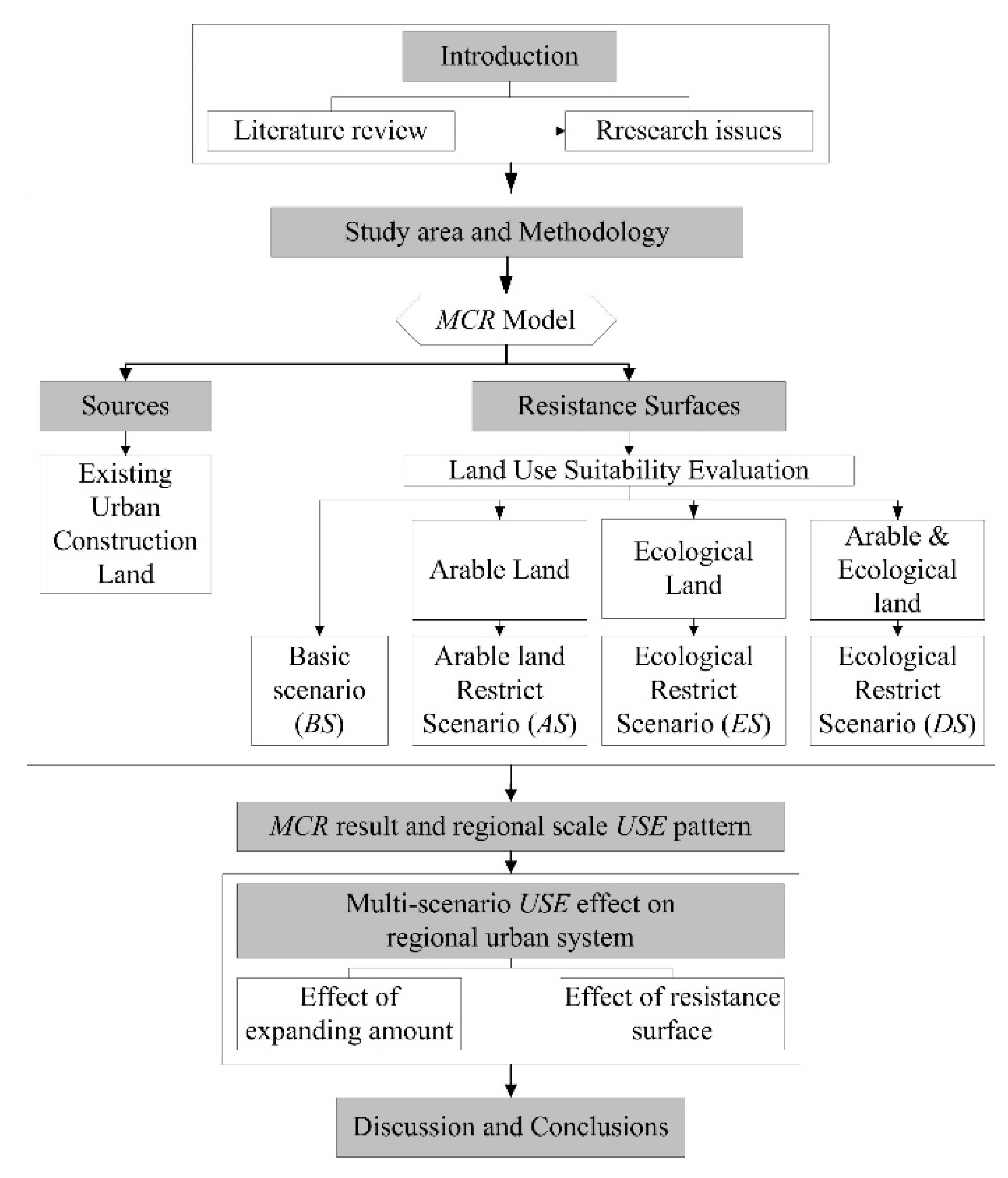
2.2. Methodologies and Data

2.2.1. USE Model

USE is a physical and socioeconomic process initially driven by human demands for space and habitable lands and is also affected by both natural and human factors [25,26]. Significant differences in landform, demographics, and economy create different types of expansion which researchers tend to classify differently [43]. Most classifications correspond to original urban patches and involve the physical diffusion process, especially at flatlands where the expansion is not limited by landform but by the development of surrounding area [44]. To this effect, location and spatial proximity are crucial factors [38,45].

As non-construction lands transform into construction ones, USE is regarded to be affected by land use suitability [27,46]. Considering the significance of spatial proximity and land use suitability, USE is similar to the migration of species and can be regarded as a physical diffusion from original settlements [38]. Mathematical models used to simulate USE include cellular automata (CA) [37,38] and the recently developed minimum cumulative resistance model (MCR) [39]. MCR was firstly designed based on landscape theory and widely used to simulate species migration from a “source” through landscapes with different resistance [47,48]. Considering the similarity between USE and species migration, the MCR model reflects spatial proximity and land use suitability factors of USE as well as constant constraints from environmental and ecological factors (e.g., species conservation areas) by defining “unusable lands” as necessary (see also understanding cost distance analysis in ArcGIS 9.3) [49]. Moreover, the MCR model has been a well-designed and widely adopted module in ArcGIS 9.3 and also has a lower data requirement, which has been proved to be feasible in simulating USE [31,49,50]. Therefore, we chose the MCR model to simulate USE under different land protection scenarios.

According to model established by Knaapen et al. [51] and modified by Yu [47], the MCR analysis can be expressed as follows:

$$\mathrm{MCR}=f_{min}{\displaystyle \sum }_{j=n}^{i=m}{D}_{ij}\times R_i$$

(1)

where f is a monotonically increasing function, D_ij is the spatial distance from landscape cell i to target patch j, and R_i is the resistance of cell i when a species travels from a source to a target patch. The MCR value reflects the minimum cumulative resistance and maximum accessibility of species to migrate, or the source-to-target spatial expansion. In USE simulation, MCR is a value that reflects minimum cumulative resistance and maximum accessibility of original urban construction lands to expand to other lands (i.e., lands with lower MCR values that are prime for transformation to urban construction lands). Accordingly, D_ij is the spatial distance of land cell i to original urban construction land j, and R_i represents the resistance of cell i in transit to urban construction land.

The MCR analysis is carried out in three steps with the cost-distance module of ArcGIS 9.3: (1) design of source as the origin; (2) design of resistance surface to determine the resistance value of every cell; and (3) calculation of the MCR value. We simulated USE with extant urban construction lands as the source, which were extracted from land use data 2010 provided by the Data Center for Resources and Environmental Science, Chinese Academy of Sciences (RESDC; http://www.resdc.cn). The resistance surfaces were designed according to different scenarios as detailed below.

2.2.2. Multi-Scenario Resistance Surface Designs

Land Use Suitability (LUS) Evaluation

As mentioned above, the MCR model was carried out with a suitable resistance surface which was designed based on the specified requirements, preferences, or predictors of certain activities [52,53]. Similar with the diffusion of species, human activities often choose lands with high possibility as potential spaces. The LUS evaluation is a method for assessing the suitability of an area for specific land use and is based on the explicit identification of constraints and opportunities for the conservation and future development of the territory [54,55,56]. In this research, it referred to the suitability of an area for land urbanization, and also indicated the suitability for the transformation to construction lands. Existing studies have provided insights on identifying the possibility of certain lands to transit to potential urban construction lands [57,58,59]. Although various complicated models have been developed to evaluate LUS [60,61], it is widely adopted that lands with proper elevation, flat topography, superior location, and traffic advantages are well suitable as potential urban construction lands [31,49]. Besides, some socio-economic indicators also reflect current status and future potential of certain lands. A well-developed area is certainly the preferred space for land development [62]. Current built-up areas wherein industry and population have already aggregated are primarily residential and can be given priority for USE [46].

Based on above discussion and also extant researches, we chose the following indicators for LUS evaluation including elevation, slope, proportion of water (POW), GDP density, population density, and traffic advantage (TA) (

Table 2. Index of land use suitability (LUS) evaluation and classification standard of affecting indicators.

Suitability Value	Elevation (M)	Slope (°)	Proportion of Water (POW)(%)	Traffic Advantage (TA)	GDP Density (RMN/Sq. Km)	Population Density (Person/Sq. Km)
5	[5, 50)	[0, 3)	[0, 5)	≥15	≥10000	≥2000
4	[50, 100)	[3, 8)	[5, 10)	[10, 15)	[5000, 10000)	[1000, 2000)
3	[100, 200)	[8, 15)	[10, 20)	[5, 10)	[2000, 5000)	[500, 1000)
2	[200, 400)	[15, 25)	[20, 50)	[2, 5)	[1000, 2000)	[200, 500)
1	≥400, or <5	[25, 90]	[50, 100]	[0, 2)	[0, 1000)	[0, 200)

). Urban construction lands were generally located at regions with lower elevation; however, flood risk should have been taken into account at certain regions as SJUA was located at a drainage concentrating region. We regarded lands lower than 5 m above sea level as unsuitable for urban construction land considering historical flood data [63,64]. Moreover, regions higher than 400 m were also less developed and regarded as protected ecological lands mostly, so they were assigned lowest suitability. The rest were reclassified into 4 levels according to the spatial distribution of extant urban construction lands. The reclassification based on slope was straightforward as the governmental standard provided a similar definition indicating that lower slope made land development easier [65]. It was difficult to carry out reclassification from the perspective of POW as water supply was essential for land development, but it was not a limiting factor in SJUA with plenty of water. On the contrary, too much water would bring an increase in the cost along with difficulty of land development [66]. Therefore, we equally divided all lands into five levels according to POW and defined those with highest POW as least suitable for land development. TA reflected accessibility and support for future spatial development, and was positively correlated with LUS [67]. Together with the integrated judgement of urban researchers from the Division of Catchment Resources/Environment and Regional Development of Nanjing Institute of Geography and Limnology, Chinese Academy of Sciences, the reclassification standard was defined according to the TA assessment result in Jiangsu Major Function Oriented Zoning (JMFOZ) (2014). GDP and population density indicated the existing support for land development, and lands with higher GDP and population were spaces in prior historical development [62,67]. They can be easily developed and are suitable lands. Other lands with high GDP and population density were of higher suitability in land development. As discussed above, the classification standards of affecting indicators are listed in Table 2.

To be specific, the elevation and slope was obtained from Digital Elevation Model (DEM) data provided by RESDC. POW was calculated with land use data 2010 (Figure 3). GDP density and population density grid data were obtained according to the distribution of construction lands and town-level GDP and population in the Statistical Year Book of Jiangsu and five prefecture-level regions in 2011 as well as the Town Population Data of the 6th National Census of China. TA data reflected the density of road networks and also their grade and location, and it was assessed in JMFOZ.

The evaluation units of chosen indicators were all 90 m × 90 m grids. Although there were many methods to integrate 6 evaluating results, we chose to multiply them with the following formula to magnify the differences among different grids:

$$V={\displaystyle \prod }_{i=1}^n{v}_i$$

(2)

where V is the calculated value of LUS of certain grid, while v_i is the suitability value obtained from single-indicator assessment; n = 6, which represents 6 selected indicators (Table 2).

As the suitability value of each indicator was from 1 to 5, the multiplication of the suitability value of six indicators was from 1 to 15,625 theoretically. However, the theoretical range was significantly broader than most existing research related to MCR simulation, such as 1–5 [50] and 1–9 [31,49]. As LUS uses relative values without specific and unchangeable assignment, we divided all grids with calculated values from 1 to 15,625 into 9 sub-groups according to existing research. The method of “Reclassification by Natural Breaks (Jenks)” in ArcGIS 9.3 was based on natural groupings inherent in the data and identified break points as per class breaks among similar values as differences between classes were maximized. After reclassification, all grids were assigned final LUS values from 1 to 9.

Resistance Surface Designs

As discussed above, higher suitability means lower resistance to USE. Thus, the grids with LUS values 1–9 were assigned resistance values 9–1 for USE. Accordingly, the resistance surface was obtained and each grid had its resistance value. It was defined as the resistance surface of the basic scenario (BS) for USE simulation.

As protection of arable lands and ecological lands were emphasized in SJUA, we conducted three other resistance surfaces based on their spatial distribution after they are converted from feature to grid (Figure 3). In the arable-land-protection scenario (AS), the grids of arable lands were erased from the BS resistance surface and the removed grids were defined “NoData” in its resistance surface. In the ecological-land-protection scenario (ES), the grids of ecological lands were erased accordingly. In the dual-land-protection scenario (DS), the grids of both arable and ecological lands were erased.

To be specific, the arable lands were the “Centralized Area of Basic Arable Lands” of Land Use Strategic Planning of Southern Jiangsu (2015–2030). The ecological lands were the “Important Ecological Function Protection Areas” in JMFOZ, and large waters including Taihu Lake, Gehu Lake, and Yangtze River were also taken as important ecological lands. Both arable and ecological lands were regarded as strictly protected lands as per extant land use regulation policies and they were not allowed to be occupied by newly added urban construction lands.

2.2.3. Calculation of USE Amounts and Urban Areas of Different Cities

With extant urban construction lands as the sources and designed four resistance surfaces, four simulated USE patterns were obtained based on MCR analysis. The results regarded every grid a certain possibility of converting to future urban construction lands, but their possibilities were different which could be indicated by their MCR values. The MCR values of a certain grids were also different under four scenarios, which reflected the different expanding patterns affected by land use regulation policies. However, it was impossible to convert the whole region to urban construction lands. In 2010, the area of urban construction lands in SJUA was about 2977 km². According to aforementioned land use strategic planning, urban and rural construction lands would increase by 2284 km² in 2030. Urban construction lands were expected to dominate the total growth while rural settlements and most towns were expected to remain stable or potentially shrink. Here, we assumed that urban construction lands will increase no more than 3000 km² and determine four USE amounts (i.e., the amount of newly added urban construction lands): 500, 1000, 2000, and 3000 km².

With the help of ArcGIS software, all grids that met the amount of corresponding area were identified based on their MCR values from low to higher under four scenarios. The identified grids were assigned to 19 cities according to their spatial connectivity with extant cities. Their allocation in 19 cities under different expanding amounts and scenarios were obtained. Accordingly, the predicted expanding amounts and final area of 19 cities were calculated.

2.2.4. Regional Scale USE Effects

The urban system is one of the most significant effects of USE at the regional scale considering land regulation and socio-economic inequity. Zipf found that the size distribution of cities follows a Pareto distribution with an exponent of unity; this concept is well-known as “Zipf’s law” or “rank-size law” [68]. When all cities in a country/region are placed in order from largest to smallest, each one has a population half the size of the preceding city [68]. Although population is primarily adopted to express the rank-size rule [69,70], other indicators may also be used to calculate the rule including area of construction lands [27,31,71].

There are two widely used indicators to describe the rank-size rule: Zipf dimension value and Pareto exponent. The former can be calculated from the Zipf formula and is expressed as follows after sorting cities from largest to smallest based on the area of urban construction lands:

$$S_i={S^{\prime }}_i\times R_i^{-q}$$

(3)

where S_i is the actual area of urban construction lands of city i (expressed in km² in this paper), S′₁ is the theoretical area of the largest city, and q is Zipf dimension value. S₁′/S₁ is the primacy index of an urban system which indicates the dominance of the largest city in the system; a higher = S₀/S₁ means a less-dominant largest city.

The rank-size distribution of regional cities can also be indicated by the Pareto law [27]:

$$G_i=A\times P_i^{-\alpha }$$

(4)

where G_i is the number of cities with area P_i or more, P_i is the area of the ith largest city, A is a constant, and α is the Pareto exponent. When α = 1, the Pareto law becomes the so-called rank-size rule. In this case, the product of a city’s rank and area is a constant equal to the area of the largest city; it indicates that the second-largest city is one-half the area of the largest, and so on. When α > 1 (or α < 1), area of cities far down in the size distribution are greater (or less) than predicted by the rank-size rule accompanied by a more (or less) even distribution of city sizes [27].

The relationship between q and α can also be determined as per the fractal characteristics of the urban system as follows [72,73]:

α × q = R²

(5)

where R² is the determination coefficient obtained from the equivalent of the Pareto law (Pareto) and Zipf formula. R² ≤ 1, so α and q cannot be greater than 1 at the same time. When R² = 1, α = q = 1 indicates that the ratio of the largest city’s area to that of the smallest city is equal to the number of all cities, or the area of ith-largest city is one-ith that of the largest city in this region. In this case, the Pareto law is in accordance with the theoretical rank-size rule. When q > 1 and α < 1, the regional urban system is of a concentrated distribution pattern wherein large cities dominate and medium and small cities are undeveloped. When q < 1 and D′ > 1, the urban system has a discrete distribution with a lower concentration of large cities and well-developed medium and small cities [74,75].

3. Results

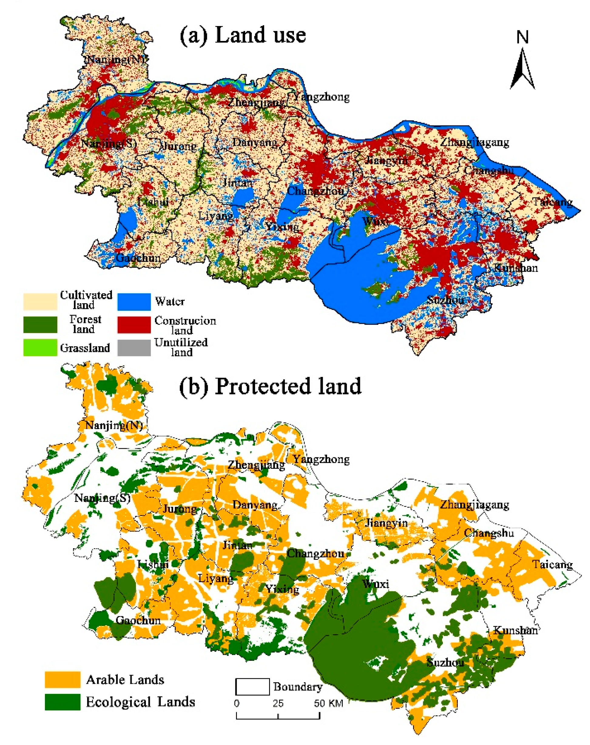
3.1. LUS Results and Resistance Surfaces by Scenarios

LUS evaluation is proved to be effective and reasonable basically as most extant urban construction lands are distributed in zones with high suitability, while most ecological lands are in zones with low suitability. Most of the SJUA is within the Yangtze River plain, which lies at a low elevation and slope and is topographically suitable for land development. There are few mountains and hills at the western and southern reaches (Figure 2; Figure 4a,b). Plenty of rivers and lakes provide sufficient water resources for regional development, but certain regions (particularly those in the center of the region) are less suitable as too high POW causes enormous costs in changing waters into buildable land (Figure 4c). As one of the most developed regions in China, SJUA is one of the national centers for both population and economy—it is comprised of preferred lands for human activities and is ripe for further development (Figure 4d,e).

As a primary support for regional development, traffic conditions are advantageous throughout the study area; areas along the Yangtze River and the surrounding Taihu Lake are better corresponding to the population and economic distribution pattern in those areas (Figure 4f). On the whole, SJUA is high suitable for land development; while mountain areas of the west and southern parts are relatively less suitable due to their higher elevation and slope (Figure 4g). Some lands close to the rivers and lakes are also less suitable due to high POW and low slope (i.e., high flood risk). City propers and their surrounding areas as well as the eastern part along the Yangtze River have a favorable development basis and high LUS (Figure 4g). These parts also have well-developed traffic infrastructures.

3.2. Comparson of Resistance Surfaces by Scenarios

Based on LUS evaluation, the obtained BS resistance surface indicated that mountains and areas near river and lakes have high resistance values, but most lands (especially those surrounding city propers) had low resistance values and were highly suitable for USE (Figure 5a). Considering AS and ES resistance surfaces, the lands of northern Nanjing, western and southern Zhenjiang, southern Wuxi and Changzhou, and northern Suzhou were “NaData” areas rife with arable and ecological lands (Figure 5b,c). DS resistance surface excluded both arable and ecological lands, so more land was prohibited from USE (Figure 5d). Under the DS scenario, more than one-half of the whole area could not be used as urban construction lands and USE was limited to the directions without arable and ecological lands. As ecological lands tend to fall into zones with higher resistance values, the number of more-resistant grids under the ES scenario decreases significantly compared to that of the BS scenario (

Table 3. Distribution of grids’ resistance value under four scenarios.

Resistance Value	Basic Scenario (BS)		Arable-Land-Protection Scenario (AS)		Ecological-Land-Protection Scenario (ES)		Dual-Land-Protection Scenario (DS)		Decreased No. of Grids Compared with BS
	No.	Proportion	No.	Proportion	No.	Proportion	No.	Proportion	AS	ES	DS
1	97966	3.02	95312	4.39	95735	3.81	93084	6.27	2654	2231	4882
2	184871	5.70	148387	6.84	179503	7.14	143614	9.67	36484	5368	41257
3	300385	9.26	195278	9.00	291241	11.58	188515	12.69	105107	9144	111870
4	270353	8.33	167273	7.71	258760	10.29	157949	10.64	103080	11593	112404
5	347941	10.72	213779	9.85	330023	13.12	198665	13.38	134162	17918	149276
6	462463	14.25	252538	11.64	428012	17.02	223257	15.03	209925	34451	239206
7	394722	12.16	211228	9.73	357707	14.22	180254	12.14	183494	37015	214468
8	532003	16.39	292645	13.49	450940	17.93	221307	14.90	239358	81063	310696
9	654669	20.17	593450	27.35	123344	4.90	78362	5.28	61219	531325	576307
total	3245373	100.00	2169890	100.00	2515265	100.00	1485007	100.00	1075483	730108	1760366

Proportion is expressed by %.

). Middle-resistance grids showed greater decreases than low- and high-resistance grids under the AS scenario. When both arable and ecological lands were taken into account, the resistance surface shrinked and about 54% of the region was unusable for USE—there was an especially significant decrease in high-resistance grids (Table 3). High-resistance grids comprised a greater proportion of total grids in BS and AS scenarios, but middle-resistance grids dominated the surface in ES and DS scenarios.

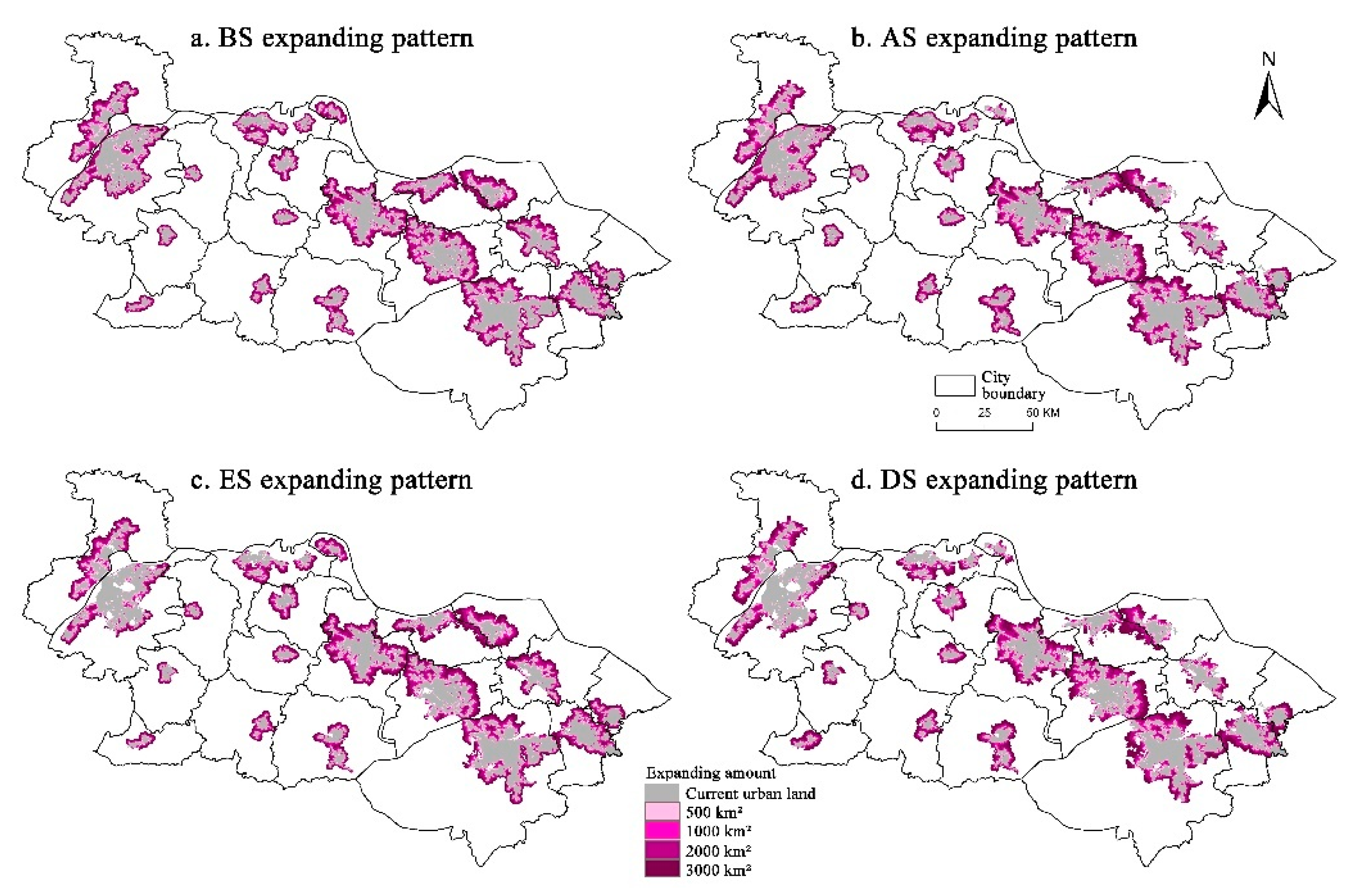
3.3. Regional Scale USE Results under Different Scenarios

MCR values increased from surrounding lands of extant urban construction lands to distant lands gradually, as USE essentially changed across lands nearer to the original urban patches to those farther away (Figure 6). As per the spatial heterogeneity of resistance values and the distribution of “No Data” grids, USE showed different patterns around different cities and in different directions (Figure 6a). Lands surrounding Taihu Lake, Yixing-Liyang Mountain, and North Nanjing had the highest MCR values not only due to their considerable distance from extant urban patches but also due to their high-resistance grids compared to extant urban construction lands. However, as arable and ecological lands were regarded as “NoData” for USE, the MCR results of AS, ES, and DS differed; protected lands were unusable for USE and thus caused disruptions in certain cities and certain directions such as the eastern part of Changzhou under the AS scenario and the eastern part of Nanjing (S) under the ES scenario (Figure 6b,c). The DS scenario encompassed both arable and ecological lands, so more unusable lands were distributed throughout the region and cities expanded in quite different patterns due to the less suitable lands among them (Figure 6d).

Different USE patterns caused significant differences in the allocation of newly added urban construction lands (Figure 7). The newly added urban construction lands surrounded extant cities in every direction when protected lands were not considered (Figure 7a). However, protected lands were spared from becoming new urban lands when arable and ecological lands were considered (Figure 7b–d). Different urban morphologies and expansion related to different resistance values and the varying distribution of unusable lands. Larger cities or those surrounded by lands with lower resistance values, such as Nanjing(S), Suzhou, Wuxi, and Changzhou, expanded faster than other cities. Under AS, ES, and DS scenarios, the USE was restricted or even blocked by arable or/and ecological lands, so the allocation of newly added urban construction lands were significantly limited (Figure 7b–d). Compared to the BS scenario, cities surrounded by more protected lands tended to have fewer allocations and their expansion was blocked in the direction of above protected lands (e.g., Wuxi, Nanjing(S), Changshu).

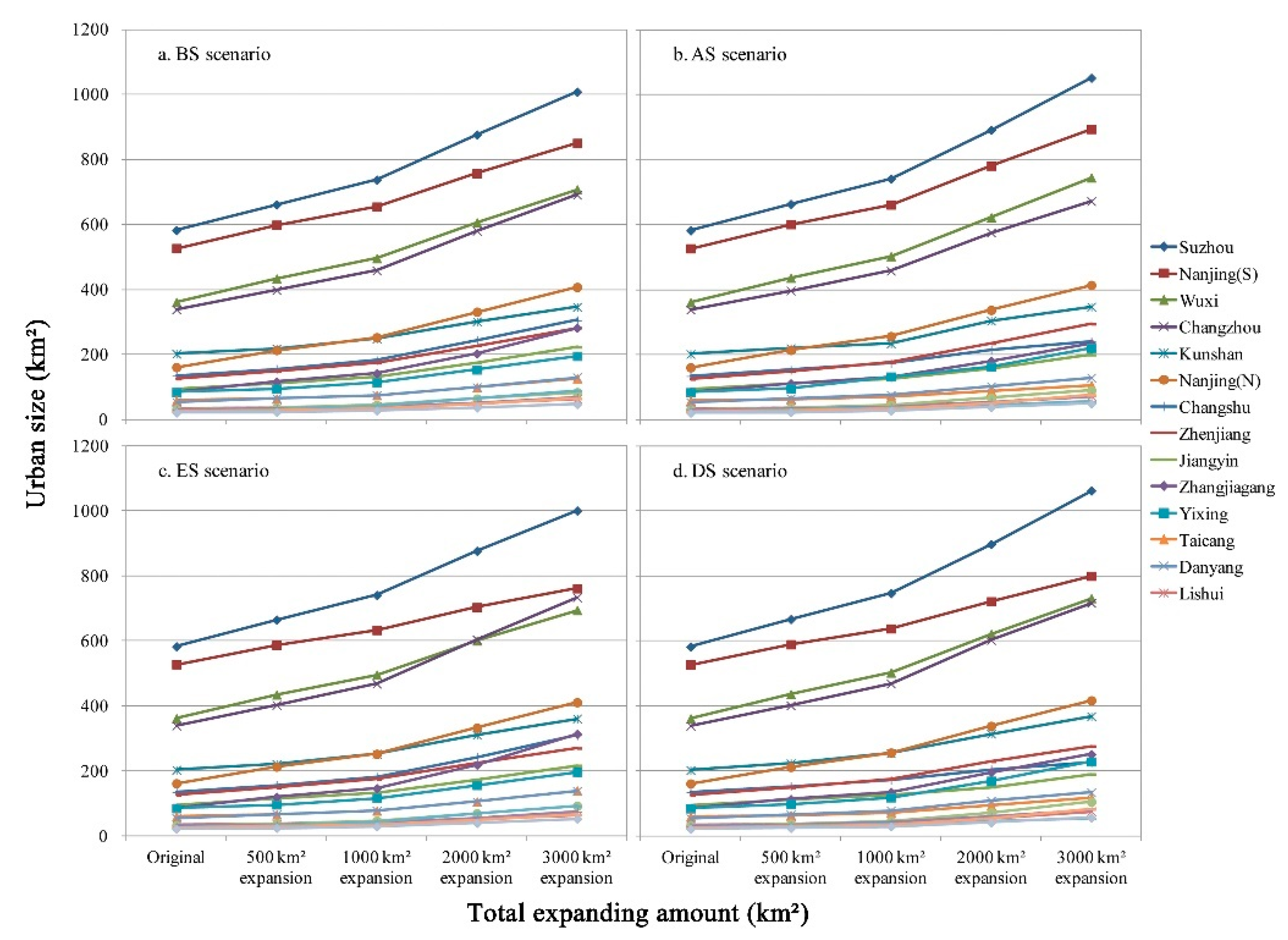
3.4. Differentiated Allocations of Newly Added Urban Construction Lands by Different USE Amount and Scenario

Similar to the USE maps above, the quantitative measurements indicated that allocations of newly added urban construction lands differed by scenario as well as expanding amount (Figure 8 and Figure 9). Larger cities tended to have higher allocations or expanded to a greater extent than smaller cities. The four largest cities in 2010 (Suzhou, Nanjing(S), Wuxi, and Changzhou) had significantly higher allocations under most scenarios. Under the BS scenario and 500 km² total amount, their expansion was 79, 72, 72 and 60 km², relatively; they used about 57% of the total newly added urban construction lands. Under other scenarios and total expanding amounts, their proportion was mostly higher than 40%. This was not, however, the case for Nanjing(N)—although it was the sixth-largest city in 2010, it consistently expanded faster than the fifth-largest city, Kunshan. The reason is that Kunshan is surrounded by more arable lands which limit its growth significantly (Figure 4g). Similar results were observed in Zhangjiagang, Danyang, and Liyang.

Considering individual cities, the differentiation was associated with both total USE amounts and expansion scenarios. At the 0–500 km² USE amount, Nanjing(S) received the greatest allocation under the AS scenario followed by BS, DS, and ES scenarios. Suzhou received its greatest allocation under the DS scenario followed by ES, AS, and BS scenarios (Figure 8a). The BS scenario favored Nanjing(S) most at the 500–1000 km² expanding amount, while Suzhou received the greatest allocation under the DS scenario (Figure 8b). As total USE amount increased, the differences in most cities’ allocations tended to increase regardless of scenario (Figure 8). For example, the difference between AS and ES scenarios of Nanjing (S) saw an increase from 14.87 km² of a 0–500 km² USE amount to 55.72 km² of a 2000–3000 km² USE amount (Supplementary Table S1).

3.5. Changes in Urban Rank-Size and Multi-Scenario Differences

Larger cities tended to grow faster, and the final area of these cities was linearly corrected with their extant sizes in 2010 (

Table 4. Correlation coefficient of urban sizes and their existing areas under four scenarios.

Total Expanding Amount (km2)		BS	AS	ES	DS
500	Linear correlation	Y = 1.144x + 3.743	Y = 1.150x + 2.790	Y = 1.138x + 4.635	Y = 1.144x + 3.738
	R2	0.997	0.998	0.997	0.997
1000	Linear correlation	Y = 1.268x + 10.618	Y = 1.278x + 8.997	Y = 1.255x + 12.644	Y = 1.270x + 10.320
	R2	0.994	0.993	0.992	0.993
2000	Linear correlation	Y = 1.485x + 29.215	Y = 1.526x + 22.880	Y = 1.447x + 35.288	Y = 1.492x + 28.245
	R2	0.985	0.988	0.975	0.978
3000	Linear correlation	Y = 1.675x + 52.178	Y = 1.759x + 38.945	Y = 1.605x + 63.164	Y = 1.701x + 48.036
	R2	0.974	0.981	0.950	0.965

). However, said linear relationship differed under the four different scenarios. The linear function slopes were greatest under the AS scenario, suggesting that large cities grew to the greatest extant under AS compared to other scenarios—the slopes were mildest under the ES scenario, where small cities expanded faster. The slopes grew increasingly steep as total USE amount increased under all four scenarios, i.e., the dominance of large cites grew increasingly high (Table 4). Larger cities grew bigger on the whole, but the existing differentiated allocations of newly added urban construction lands related to both increasing expanding amount and scenario still caused significant differences in urban rank-size in the study area.

Suzhou was the largest city in 2010 followed by Nanjing(S). They consistently dominated other cities in terms of size regardless of USE amount and expanding scenario (Figure 9). The third- and fourth-largest cities changed in the ES scenario when total USE amount reached 3000 km²: Changzhou took the place of Wuxi as the third largest city. Similarly, Nanjing(N), Zhangjiagang, and some other cities changed rank under this scenario as total expanding amount increased (Figure 9c). Nanjing(N) and Zhangjiagang, in fact, changed ranks under all other scenarios; Zhenjiang changed under the AS scenario and Yixing did so under the DS scenario. Across four scenarios, the ranks of medium cities changed more fluently while those of large and small cities’ remained more stable.

The reliable fractal characteristics (with R² values of about 0.90;

Table 5. Urban rank-size of regional urban system under different scenarios.

Total Expanding Amount (km2)	Scenario	S1	S1’	S1’/S1	q	α	R2
Original	/	582.78	1268.51	2.18	1.27	0.72	0.91
500 km2	BS	662.00	1478.22	2.23	1.27	0.71	0.90
	AS	738.31	1634.18	2.21	1.24	0.73	0.90
	ES	877.16	1893.52	2.16	1.18	0.75	0.89
	DS	1008.89	2101.05	2.08	1.12	0.79	0.88
1000 km2	BS	664.32	1488.90	2.24	1.27	0.71	0.90
	AS	742.37	1642.53	2.21	1.24	0.72	0.90
	ES	892.41	1932.16	2.17	1.19	0.75	0.90
	DS	1052.35	2158.12	2.05	1.14	0.79	0.90
2000 km2	BS	664.73	1472.32	2.21	1.26	0.71	0.90
	AS	740.74	1610.98	2.17	1.23	0.73	0.90
	ES	876.60	1833.34	2.09	1.15	0.77	0.89
	DS	1000.56	2012.22	2.01	1.09	0.81	0.88
3000 km2	BS	667.06	1477.48	2.21	1.27	0.71	0.91
	AS	746.75	1629.93	2.18	1.24	0.73	0.90
	ES	897.69	1868.69	2.08	1.17	0.77	0.90
	DS	1062.75	2050.00	1.93	1.10	0.82	0.90

) confirmed the above results. It was indicated that q was always higher than 1.1, but α was lower than 0.8; this proved large cities dominated the regional urban system under all scenarios. However, q decreased and α increased gradually under each scenario as total USE amount increased. Both variables became closer to one as the expansion of large cities decelerated while medium and small cities begun to expand faster. In other words, the urban system continually grew more balanced. The values of q and α were different related to the four scenarios, and the differences became greater with increasing USE amounts. Both q and α were closest to one under the ES scenario, indicating that protection on ecological lands limited the expansion of large cities more efficiently. Medium and small cities expanded significantly faster under the AS scenario as q and α were both farthest from one, especially at the USE amounts of 2000 and 3000 km².

Although large cities were of dominance under all scenarios, the primary ratios of the largest city, i.e., Suzhou, were not too high indicated by the lower actual area than its theoretical area (Table 5). The primacy ratios also tended to decrease as USE amount increased, indicating a decreasing proportion of Suzhou’s area of urban construction lands to the total of SJUA. The primacy ratios were also scenario-related; those of the DS scenarios were consistently the lowest. In effect, growth in the largest city was limited to a certain extent. Suzhou’s primary ratio was highest in the BS scenario, i.e., when there were no land-protection policies set.

4. Discussion

Regional scale USE is always uneven among various cities due to different location, topography, resource-carrying capacity, governmental regulations, and a myriad of other factors [38,69]. Uneven USE causes imbalanced economic development across the region [22,76] and profoundly affects regional ecological safety [31,77]. Former researchers have focused on the history and status quo of regional scale USE and its social, economic, and environmental effects [78,79]. Few have attempted to project certain insights or policy recommendations into future USE scenarios. Land, the primary resource supporting such expansion, should also be carefully considered in terms of availability and suitability. Uneven USE and land regulation policies are very important—especially in rapidly developing China, where these issues have garnered increasing attention as their profound socio-economic and ecological effects. China’s ambition for improving global competitiveness and promoting new urbanization is pressed for developing dozens of national, regional and local UAs in coming decades [23]. As a unit of several cities with complex interactions, the UA is suitable for regional scale USE simulation and reflects the patterns and also effects of uneven USE. We chose SJUA for regional scale USE research accordingly, as its uneven development pattern has affected its regional urban system in ways that can be readily observed.

4.1. Feasibility of the MCR Model in Regional Scale USE Simulations

Regional scale USE simulation is the basis for regulating and optimizing sustainable UA development [23]. However, regional scale USE differs markedly from that of an individual city; it has several sources and is significantly affected by the allocations of newly added urban construction lands. USE is both a physical and socioeconomic process of urban land diffusion which involves spatial proximity and land use suitability [31,48]. The MCR model is a useful tool for simulating the spatial expansion of several disparate cities as they diffuse across a given region. Its feasibility is not only proved by the increasing adoption by other researchers [31,49,50], but also the consistency between predicted USE pattern and the extant one in SJUA. With urban construction lands in 2005 and land use suitability as the input variables in the MCR model, the simulated pattern of urban construction lands in 2010 is highly consistent with the actual pattern in 2010 and about 84% of the construction lands are the same.

Urban development is a continuous process with certain rules; the formation of a certain pattern is the result of long-term development, which would continue when no decisive promoting or restricting factors are proposed [12]. In the showed results, the predicted area of these cities was linearly corrected with their extant sizes in 2010, indicating the rationality of the simulated result and also the feasibility of adopted MCR model. It was further proved by the comparison with previous research which had made similar observations. For example, Liu et al. found that Suzhou, Wuxi, Nanjing, and Changzhou expanded to the greatest extent over the study region during the years 1980 to 2010 [80]; these cities have also received the greatest allocations of urban lands. The rank-size patterns here are also similar to the result of Li and Sun obtained from data before 2007, where S₁′/S₁ was always higher than 2 [29].

The MCR model was feasible in its convenience in dealing with complicated expanding scenarios. In this research, the edge-expansion of original urban patches was predominant [80], which was also the common phenomenon in other regions—especially flatlands, which have relatively few topographical limitations [81]. However, some newly added and relatively isolated urban patches might appear during rapid urbanization. The MCR model could provide the convenience by adding new urban patches to “sources”, which would expand together with other cities. Moreover, if more restricted lands were not allowed to be occupied by urban expansion, it was easy to erase them from the resistance surface, or assign them a significantly higher resistance value to build barriers for urban expansion. There was research emphasizing the importance of land ownership in affecting urban expansion, especially in some countries where private lands might form the barrier for urban expansion [82]. However, part of the lands surrounding extant cities are state-owned, while the rest are owned by rural collective economic organizations and could be turned into state-owned ones easily in China [83]. The property restriction is not so strong for state-owned lands, so the effect of ownership is not emphasized in China. For those where land ownership is more significant, the private lands could to be erased from the resistance surface as unusable lands for urban expansion.

4.2. USE Patterns, Effects of Land Protection Policies on Regional Urban Systems

As discussed above, the spatial patterns of USE were basically a direct enlargement of original city sizes in the given region, so the rank-size of most cities is basically similar under increasing expanding amounts. Basically, the patterns in this study are not only consistent with historical data, but also with findings in other urban agglomerations and similar areas [27,84,85]. However, different USE amount and scenarios do induce changes to spatial patterns.

There were no limitations under the BS scenario, where LUS was the only factor that affected USE. Larger cities are surrounded by greater areas of suitable lands and tend to expand faster and grow larger than smaller ones. Considering historical development, large cities also obtain greater opportunities for growing larger. Suzhou, the region’s largest city, is close to one of China’s economic centers—Shanghai and benefitted from industrial transfers which promote its economic development and population agglomeration, and more urban construction lands are needed to support its development [27,86]. Nanjing has an administrative advantage as the provincial capital of Jiangsu, which has given it priority in terms of economic development and land resource allocation [22]. Other large cities are mostly prefecture-level propers, while medium and small cities are mostly far away from city propers and are with lower administrative level.

The power of allocating urban construction lands is usually controlled by the provincial government; larger cities are more likely to receive greater allocations as per their inherently greater demands for space [75]. Large cities also often have priority in terms of regional development, so the government may also allocate them more land and promote their regional competitiveness [27,34]. These priorities have caused so-called “agglomeration shadows” in new economic geography, which predicts that spatial development will become increasingly centralized as locational patterns persist over time due to self-reinforcement [87]. Small cities that are far away from larger ones, conversely, might grow slowly or even shrink [88]. Although none of the cities in this study decreased in size, the possibility should not be neglected and targeted land regulation policies are needed to deal with this.

Various land protection policies impose certain limitations to USE. The amounts, and especially, spatial distributions of protected lands designated as “unusable” affect USE by setting up different barriers. In China, the central government suggested protecting arable and ecological lands and various policies have been proposed. The scenarios in this study were indeed based on such land protection policies; AS, ES, and DS scenarios which define certain areas as “unusable land” for USE and thus affect the land allocations and cities’ rank-size in SJUA. The general patterns of regional urban system do not change significantly in these scenarios versus the BS scenario, but the dominance of larger cities tends to decrease as medium and small cities expand faster when given greater expanding amounts. The AS scenario is the one that most favors the expansion of large cities, while ES scenario least favors that. It indicates that the protection of arable lands promotes the expansion of large cities. Their growth is maximally restricted when ecological lands are taken into account.

4.3. More Effective Spatial Distribution of Protected Lands

Surrounding arable lands are an important source of newly added urban construction lands in China [89]. The Disciplines on Determining Permanent Basic Arable Lands of Ministry of Lands and Resources of China aims to protect food safety and control USE in cities by delineating strictly protected arable lands surrounding large cities in the future. However, the AS scenario does not effectively control the expansion of large cities or promote the development of medium and small cities to this effect. Therefore, more arable lands surrounding large cities should be protected than in other parts of the country [8]. The ES scenario makes larger cities less dominant while favoring the growth of medium and small cities—this scenario represents the more effective ecological land protection policy. Ecological land is a major component of a “green belt”, where USE is limited to maintain ecosystem function and environmental quality; many large cities in the study area lie adjacent to a green belt [90]. Arable lands have multi-functionality as an important component of SJUA’s green belt and thus merit a higher amount and more optimized spatial distribution [8]. It is also indicated that similarity among cities’ rank-size patterns is accompanied by significant differences in certain cities as per their land allocations. The results reflect the real-world effects of land protection policies on the spatial expansion of individual cities, and suggest that the growth of certain cities can be effectively regulated if surrounding protected lands are spatially optimized.

5. Conclusions

With the support of MCR model and under the context of various land protection policies, the possibility of future USE and induced changes of urban systems were detected here. It was indicated that the MCR model could effectively be adopted to simulate regional scale USE as the simulation results were in accordance with the historical development of different cities and also urban systems in SJUA. Theoretically, extant urban construction lands were the source of future expansion and LUS was the primary factor affecting the possibility of converting to urban construction lands; both factors form the technological basis of the MCR model. Future USE appeared to be linearly corrected with extant city size; the larger a city is currently, the more likely it was to grow faster than other cities on the whole. However, few cities expanded at unconventional speed and fluctuated to a varying extent, which needs to be explored further.

The land protection policies indeed affected the spatial pattern of USE and also the regional urban system to a certain extent. The effect of land protections varied according to their spatial distributions. Arable land protection favored the growth of large cities, but ecological land protection basically facilitated the expansion of medium and small cities. Policy makers would do better to emphasize spatial distribution in addition to the total amount of protected land based on the expectation of future regional development pattern. In this study, arable land protection did not bring wanted effect on controlling the unlimited growth of big cities, and the reason might be that there was not enough arable land distributed at the surrounding areas of big cities. Therefore, it was suggested that arable land at the suburbs of big cities should be strictly protected. It would control the unlimited expansion of big cities and also provide greater opportunities for medium and small cities effectively.

In conclusion, this research not only provided more possibility on how to regulate regional level USE and ways to realize it, but it also gave suggestions on how to make the distribution of protected lands more reasonable by optimizing the orientation of land use policies. Aiming at bettering land use efficiency and promoting sustainable land development, our research provided valuable perspective, feasible technology and also optional proposals. However, there were still some limitations, and the first one related to the design of resistance surfaces with resistance values from one to nine. Although the assignment was relatively rational, it still lacked scientific inadequacy. More practical expanding processes should be analyzed to detect more explicit resistance values. Secondly, regional scale expansion is a complicated process of a group of cities, and their interactions should be considered through the modification of the MCR model.

References

1. Bai, X.; Shi, P.; Liu, Y. Realizing China’s urban dream. Nature 2014, 509, 158–160. [Google Scholar] [CrossRef]
2. Seto, K.C.; Fragkias, M.; Güneralp, B.; Reilly, M.K. A meta-analysis of global urban land expansion. PLoS ONE 2011, 6, e23777. [Google Scholar] [CrossRef] [PubMed]
3. Deng, Y.; Liu, Y.; Fu, B. Urban growth simulation guided by ecological constraints in Beijing city: Methods and implications for spatial planning. J. Environ. Manag. 2019, 243, 402–410. [Google Scholar] [CrossRef]
4. Yang, C.; Li, Q.; Hu, Z.; Chen, J.; Shi, T.; Ding, K.; Wu, G. Spatiotemporal evolution of urban agglomerations in four major bay areas of US, China and Japan from 1987 to 2017: Evidence from remote sensing images. Sci. Total Environ. 2019, 671, 232–247. [Google Scholar] [CrossRef] [PubMed]
5. Fei, W.; Zhao, S. Urban land expansion in China’s six megacities from 1978 to 2015. Sci. Total Environ. 2019, 664, 60–71. [Google Scholar] [CrossRef] [PubMed]
6. Gao, J.; Wei, Y.D.; Chen, W.; Chen, J. Economic transition and urban land expansion in provincial China. Habitat Int. 2014, 44, 461–473. [Google Scholar] [CrossRef]
7. Long, Y.; Wu, K. Simulating block-level urban expansion for national wide cities. Sustainability 2017, 9, 879. [Google Scholar] [CrossRef]
8. McDonnell, M.J.; Picket, S.T.A. Ecosystem structure and function along urban-rural gradients: An unexploited opportunity for ecology. Ecology 1990, 71, 1232–1237. [Google Scholar] [CrossRef]
9. Xu, G.; Jiao, L.; Liu, J.; Shi, Z.; Zeng, C.; Liu, Y. Understanding urban expansion combining macro patterns and micro dynamics in three Southeast Asian megacities. Sci. Total Environ. 2019, 660, 375–383. [Google Scholar] [CrossRef]
10. Losiri, C.; Nagai, M.; Ninsawat, S.; Shrestha, R.P. Modeling urban expansion in Bangkok Metropolitan region using demographic-economic data through Cellular Automata-Markov Chain and Multi-Layer Perceptron-Markov Chain models. Sustainability 2016, 8, 686. [Google Scholar] [CrossRef]
11. Lu, H.; Zhang, M.; Sun, W.; Li, W. Expansion analysis of Yangtze River Delta Urban Agglomeration using DMSP/OLS nighttime light imagery for 1993 to 2012. Int. J. Geo Inf. 2018, 7, 52. [Google Scholar] [CrossRef]
12. Che, Q.; Duan, X.; Guo, Y.; Wang, L.; Cao, Y. Urban spatial expansion process, pattern and mechanism in Yangtze River Delta. Acta Geogr. Sin. 2011, 66, 446–456. (In Chinese) [Google Scholar]
13. Rodgers, S. Urban geography: Urban growth machine. In The International Encyclopedia of Human Geography; Kitchin, R., Thrift, N., Eds.; Elsevier: Oxford, UK, 2009; Volume 12, pp. 40–45. [Google Scholar]
14. Rodrigue, J. The Geography of Transport Systems (FOURTH EDITION); Routledge: New York, NY, USA, 2017. [Google Scholar]
15. Wei, Y.D.; Ye, X. Urbanization, urban land expansion and environmental change in China. Stoch. Environ. Res. Risk Assess. 2014, 28, 757–765. [Google Scholar] [CrossRef]
16. Angel, S.; Parent, J.; Civco, D.L.; Blei, A.M. The Persistent Decline of Urban Densities: Global and Historical Evidence of Sprawl; Lincoln Institute Working Paper; Lincoln Institute of Land Policy: Cambridge, MA, USA, 2010. [Google Scholar]
17. Long, Y.; Zhai, W.; Shen, Y.; Ye, X. Understanding uneven urban expansion with natural cities using open data. Landsc. Urban Plan. 2018, 177, 281–293. [Google Scholar] [CrossRef]
18. Ye, X.; Xie, Y. Re-examination of Zipf’s law and urban dynamic in China: A regional approach. Ann. Reg. Sci. 2012, 49, 135–156. [Google Scholar] [CrossRef]
19. Lu, S.; Guan, X.; He, C.; Zhang, J. Spatio-temporal patterns and policy implications of urban land expansion in Metropolitan Areas: A case study of Wuhan Urban Agglomeration, Central China. Sustainability 2014, 6, 4723–4748. [Google Scholar] [CrossRef]
20. Ding, C.; Zhao, X. Assessment of urban spatial-growth patterns in China during rapid urbanization. Chin. Econ. 2011, 44, 46–71. [Google Scholar] [CrossRef]
21. World Bank. World Development Indicators 2016; World Bank: Washington, DC, USA, 2016. [Google Scholar] [CrossRef]
22. Wei, Y.D.; Li, H.; Yue, W. Urban land expansion and regional inequality in transitional China. Landsc. Urban Plan. 2017, 163, 17–31. [Google Scholar] [CrossRef]
23. Fang, C.; Yu, D. Urban agglomeration: An evolving concept of an emerging phenomenon. Landsc. Urban Plan. 2017, 162, 126–136. [Google Scholar] [CrossRef]
24. Gottmann, J. Megaoloplis: The Urbanized Northeastern Seaboard of the United States; The MLT Press: Cambridge, MA, USA, 1961. [Google Scholar]
25. McGee, T.G. The Emergence of Desakota Regions in Asia: Expanding a Aypothesis; University of Hawaii Press: Honolulu, HI, USA, 1991. [Google Scholar]
26. Gao, X.; Xu, Z.; Niu, F.; Long, Y. An evaluation of China’s urban agglomeration development from the spatial perspective. Spat. Stat. 2017, 21, 475–491. [Google Scholar] [CrossRef]
27. Tian, G.; Jiang, J.; Yang, Z.; Zhang, Y. The urban growth, size distribution and spatio-temporal dynamic pattern of the Yangtze River Delta megalopolitan region, China. Ecol. Model. 2011, 222, 865–878. [Google Scholar] [CrossRef]
28. Yu, G.; Li, M.; Xu, L.; Tu, Z.; Yu, Q.; Yang, D.; Xie, Y.; Yang, Y. A theoretical framework of urban systems and their evolution: The GUSE theory and its simulation test. Sustain. Cities Soc. 2018, 41, 792–801. [Google Scholar] [CrossRef]
29. Li, P.; Sun, W. Pattern and driving mechanism of urban expansion of Southern Jiangsu province since reform and opening up. Resour. Environ. Yangtze Basin 2013, 22, 1529–1536. (In Chinese) [Google Scholar]
30. Angel, S.; Parent, J.; Civco, D.L.; Blei, A.; Potere, D. The dimensions of global urban expansion: Estimates and projections for all countries, 2000–2050. Prog. Plan. 2011, 75, 53–107. [Google Scholar] [CrossRef]
31. Li, P.; Fan, J. Scenario simulation of regional urban expansion and effects on urban form and system: A case study of Xijiang River Economic Belt in Guangxi. Geogr. Res. 2014, 33, 509–519. (In Chinese) [Google Scholar]
32. Fang, S.; Gertner, G.Z.; Sun, Z.; Anderson, A.A. The impact of interactions in spatial simulation of the dynamics of urban sprawl. Landsc. Urban Plan. 2005, 73, 294–306. [Google Scholar] [CrossRef]
33. Poelmans, L.; Van Rompaey, A. Complexity and performance of urban expansion models. Comput. Environ. Urban Syst. 2010, 34, 17–27. [Google Scholar] [CrossRef]
34. Batty, M. Cities, prosperity, and the importance of being large. Environ. Plan. B 2011, 38, 385–387. [Google Scholar] [CrossRef]
35. Batty, M.; Xie, Y.; Sun, Z. Modeling urban dynamics through GIS-based cellular automata. Comput. Environ. Urban Syst. 1999, 23, 205–233. [Google Scholar] [CrossRef]
36. Matthews, R.B.; Gilbert, N.G.; Roach, A.; Polhill, J.G.; Gotts, N.M. Agent-based land-use models: A review of applications. Landsc. Ecol. 2007, 22, 1447–1459. [Google Scholar] [CrossRef]
37. Li, X.; Yeh, A.G. Modelling sustainable urban development by the integration of constrained cellular automata and GIS. Int. J. Geogr. Inf. Sci. 2000, 14, 131–152. [Google Scholar] [CrossRef]
38. Li, L.; Sato, Y.; Zhu, H. Simulating spatial urban expansion based on a physical process. Landsc. Urban Plan. 2003, 64, 67–76. [Google Scholar] [CrossRef]
39. Wang, H.; Peng, P.; Kong, X.; Zhang, T.; Yi, G. Evaluating the suitability of urban expansion based on the Logic Minimum Cumulative Resistance Model: A case study from Leshan, China. Int. J. Geo Inf. 2019, 8, 291. [Google Scholar] [CrossRef] [Green Version]
40. Vermeiren, K.; Vanmaercke, M.; Beckers, J.; Van Rompaey, A. ASSURE: A model for the simulation of urban expansion and intra-urban social segregation. Int. J. Geogr. Inf. Sci. 2016, 30, 2377–2400. [Google Scholar] [CrossRef]
41. Zhong, T.; Chen, Y.; Huang, X. Impact of land revenue on the urban land growth toward decreasing population density in Jiangsu Province, China. Habitat Int. 2016, 58, 34–41. [Google Scholar] [CrossRef]
42. Wang, L.; Wong, C.; Duan, X. Urban growth and spatial restructuring patterns: The case of Yangtze River Delta Region, China. Environ. Plan. B 2016, 43, 515–539. [Google Scholar] [CrossRef]
43. Roberto, C.; Maria, C.G.; Paolo, R. Urban mobility and urban form: The social and environmental cost of different patterns of urban expansion. Ecol. Econ. 2002, 40, 192–216. [Google Scholar] [CrossRef]
44. Gomes, E.; Banos, A.; Abrantes, P.; Rocha, J. Assessing the effect of spatial proximity on urban growth. Sustainability 2018, 10, 1308. [Google Scholar] [CrossRef] [Green Version]
45. Kasraian, D.; Maat, K.; van Wee, B. The impact of urban proximity, transport accessibility and policy on urban growth: A longitudinal analysis over five decades. Environ. Plan. B 2019, 46, 1000–1017. [Google Scholar] [CrossRef] [Green Version]
46. Ullah, K.M.; Mansourian, A. Evaluation of land suitability for urban land-use planning: Case study Dhaka City. Trans. GIS 2016, 20, 20–37. [Google Scholar] [CrossRef]
47. Yu, K. Security patterns and surface model and in landscape planning. Landsc. Urban Plan. 1996, 36, 1–17. [Google Scholar] [CrossRef]
48. Adriaensen, F.; Chardona, J.P.; De Blust, G.; Swinnen, E.; Villalba, S.; Gulinck, H.; Matthysen, E. The application of ‘least-cost’ modelling as a functional landscape model. Landsc. Urban Plan. 2003, 64, 233–247. [Google Scholar] [CrossRef]
49. Ye, Y.; Su, Y.; Zhang, H.; Liu, K.; Wu, Q. Construction of an ecological resistance surface model and its application in urban expansion simulations. J. Geogr. Sci. 2015, 25, 211–224. [Google Scholar] [CrossRef]
50. Li, X.; Wang, M.; Liu, X.; Chen, Z.; Wei, X.; Che, W. MCR-modified CA–Markov model for the simulation of urban expansion. Sustainability 2018, 10, 3116. [Google Scholar] [CrossRef] [Green Version]
51. Knaapen, J.P.; Scheffer, M.; Harms, B. Estimating habitat isolation in landscape planning. Landsc. Urban Plan. 1992, 23, 1–16. [Google Scholar] [CrossRef]
52. Collins, M.G.; Steiner, F.R.; Rushman, M.J. Land-use suitability analysis in the United States: Historical development and promising technological achievements. Environ. Manag. 2001, 28, 611–621. [Google Scholar] [CrossRef] [PubMed]
53. Malczewski, J. GIS-based land-use suitability analysis: A critical overview. Prog. Plan. 2004, 62, 3–65. [Google Scholar] [CrossRef]
54. FAO. A Framework for Land Evaluation; FAO: Rome, Italy; UN: New York, NY, USA, 1976; Available online: http://www.fao.org/3/X5310E/X5310E00.htm (accessed on 9 November 2019).
55. FAO. Guidelines for Land-Use Planning; FAO: Rome, Italy; UN: New York, NY, USA, 1993; Available online: https://www.mpl.ird.fr/crea/taller-colombia/FAO/AGLL/pdfdocs/guidelup.pdf (accessed on 9 November 2019).
56. Steiner, F. Resource suitability: Methods for analysis. Environ. Manag. 1983, 7, 401–420. [Google Scholar] [CrossRef]
57. Pereira, J.M.C.; Duckstein, L. A multiple criteria decision-making approach to GIS-based land suitability evaluation. Int. J. Geogr. Inf. Syst. 1993, 7, 407–424. [Google Scholar] [CrossRef]
58. Jankowski, P.; Richard, L. Integration of GIS-based suitability analysis and multicriteria evaluation in a spatial decision support system for route selection. Environ. Plan. B 1994, 21, 326–339. [Google Scholar] [CrossRef]
59. Li, C.; Zhao, J.; Xu, Y. Examining spatiotemporally varying effects of urban expansion and the underlying driving factors. Sustain. Cities Soc. 2017, 28, 307–320. [Google Scholar] [CrossRef]
60. Doygun, H.; Alphan, H.; Gurun, D.K. Analysing urban expansion and land use suitability for the city of Kahramanmaraş, Turkey, and its surrounding region. Environ. Monit. Assess. 2008, 145, 387–395. [Google Scholar] [CrossRef] [PubMed]
61. Yan, Y.; Zhou, R.; Ye, X.; Zhang, H.; Wang, X. Suitability evaluation of urban construction land based on an approach of vertical-horizontal processes. Int. J. Geo Inf. 2018, 7, 198. [Google Scholar] [CrossRef] [Green Version]
62. Tang, C.; Fan, J.; Sun, W. Distribution characteristics and policy implications of territorial development suitability of the Yangtze River Basin. J. Geogr. Sci. 2015, 25, 1377–1392. [Google Scholar] [CrossRef]
63. Chen, W.; Sun, W.; Duan, X.; Chen, J. Regionalization of potential land use in Jiangsu Province under eco-economic approach. Sci. Geogr. Sin. 2007, 27, 312–317. (In Chinese) [Google Scholar]
64. Yu, G.; Hu, S.; Li, C. Study on historical extreme floods in occurrence year and floody height, Taihu. Quaternary Sci. 2013, 33, 167–178. (In Chinese) [Google Scholar]
65. Dang, L.; Xu, Y.; Tang, Q.; Zhao, H.; Yang, B.; Sun, G. Potential and spatial distribution of suitable construction land along the Xijiang Riverside in Guangxi. J. Nat. Resour. 2014, 29, 387–398. (In Chinese) [Google Scholar]
66. Chen, W.; Sun, W.; Duan, X.; Chen, J. Regionalization of regional potential development in Suzhou City. Acta Geogr. Sin. 2006, 61, 839–846. (In Chinese) [Google Scholar]
67. Fan, J. Draft of major function oriented zoning of China. Acta Geogr. Sin. 2015, 70, 186–201. (In Chinese) [Google Scholar]
68. Zipf, G.K. Human Behavior and the Principle of Least Effort; Addison-Wesley Press: Oxford, UK, 1949. [Google Scholar]
69. Song, S.; Zhang, K.H. Urbanisation and city size distribution in China. Urban Stud. 2002, 39, 2317–2327. [Google Scholar] [CrossRef]
70. Decker, E.H.; Kerkhoff, A.J.; Moses, M.E. Global patterns of city size distributions and their fundamental drivers. PLoS ONE 2007, 9, e934. [Google Scholar] [CrossRef] [PubMed]
71. Tan, M.; Lv, C. Distribution of China city size expressed by urban built-up area. Acta Geogr. Sin. 2003, 58, 285–293. (In Chinese) [Google Scholar]
72. Wu, Z.; Dai, X.; Yang, W. On reconstruction of Pareto formal and its relationship with development of urban system. Hum. Geogr. 2000, 15, 15–19. (In Chinese) [Google Scholar]
73. Yue, W.; Xu, J. Application of fractal geometry theory in the study of human geography. Geogr. Territ. Res. 2001, 17, 48–53. (In Chinese) [Google Scholar]
74. Carroll, G.R. National city-size distribution: What do we know after 67 years of research? Prog. Hum. Geogr. 1982, 6, 1–43. [Google Scholar] [CrossRef]
75. Sun, Z.; Yuan, Y.; Wang, Y.; Zhang, X. Research on city-size distribution and allometric growth in Jiangsu Province based on fractal theory. Geogr. Res. 2011, 30, 2162–2171. (In Chinese) [Google Scholar]
76. Alonso, W. Urban and regional imbalances in economic development. Econ. Dev. Cult. Chang. 1968, 17, 1–14. [Google Scholar] [CrossRef]
77. Squire, G.D. Urban Sprawl and the Uneven Development of Metropolitan America in Urban Sprawl: Causes, Consequences and Policy Responses; Urban Institute Press: Washington, DC, USA, 2002. [Google Scholar]
78. He, C.; Okada, N.; Zhang, Q.; Shi, P.; Li, J. Modelling dynamic urban expansion processes incorporating a potential model with cellular automata. Landsc. Urban Plan. 2008, 86, 79–91. [Google Scholar] [CrossRef]
79. Jafari, M.; Majedi, H.; Monavari, S.M.; Alesheikh, A.A.; Zarkesh, M.K. Dynamic simulation of urban expansion through a CA-Markov model Case study: Hyrcanian region, Gilan, Iran. Eur. J. Remote Sens. 2016, 49, 513–529. [Google Scholar] [CrossRef] [Green Version]
80. Liu, G.; Zhang, L.; Zhang, Q. Urban expansion and landscape pattern analysis in the Southern Jiangsu, China. Resour. Environ. Yangtze Basin 2014, 23, 1375–1382. (In Chinese) [Google Scholar]
81. He, Q.; Song, Y.; Liu, Y.; Yin, C. Diffusion or coalescence? Urban growth pattern and change in 363 Chinese cities from 1995 to 2015. Sustain. Cities Soc. 2017, 35, 729–739. [Google Scholar] [CrossRef]
82. Kline, J.D.; Azuma, D.L.; Alig, R.J. Population growth, urban expansion, and private forestry in Western Oregon. For. Sci. 2004, 50, 33–43. [Google Scholar] [CrossRef]
83. Liu, Y.S.; Fang, F.; Li, Y.H. Key issues of land use in China and implications for policy making. Land Use Policy 2014, 40, 6–12. [Google Scholar] [CrossRef]
84. Chen, X.; Greene, R. The spatial-temporal dynamics of China’s changing urban hierarchy (1950–2005). Urban Stud. Res. 2012, 2012, 162965. [Google Scholar] [CrossRef]
85. Fang, C.; Wang, Z. Quantitative diagnoses and comprehensive evaluations of the rationality of Chinese urban development patterns. Sustainability 2015, 7, 3859–3884. [Google Scholar] [CrossRef] [Green Version]
86. Gao, J.; Wei, Y.D.; Chen, W.; Yenneti, K. Urban land expansion and structural change in the Yangtze River Delta, China. Sustainability 2015, 7, 10281–10307. [Google Scholar] [CrossRef] [Green Version]
87. Krugman, P. Increasing returns and economic geography. J. Polit. Econ. 1991, 99, 483–499. [Google Scholar] [CrossRef]
88. Partridge, M.D.; Rickman, D.S.; Ali, K.; Rose Olfert, M. Do New Economic Geography agglomeration shadows underlie current population dynamics across the urban hierarchy? Pap. Reg. Sci. 2009, 88, 445–466. [Google Scholar] [CrossRef]
89. Tan, M.; Zhu, H.; Liu, L.; Guo, G. Spatial patterns of built-up areas around Beijing. Acta Geogr. Sin. 2007, 62, 861–869. [Google Scholar]
90. Munton, R.J.C. London’s Green Belt: Containment in Practice; Routledge: London, UK, 2006. [Google Scholar]
Figure 1. Flowchart of detection procedures.
Ijgi 08 00521 g001
Figure 2. Location, administrative divisions and topography of Southern Jiangsu Urban Agglomeration (SJUA).
Ijgi 08 00521 g002
Figure 3. Land use (a) and spatial distribution of arable and ecological lands (b).
Ijgi 08 00521 g003
Figure 4. The distribution patterns of six indicators and LUS.
Ijgi 08 00521 g004
Figure 5. Resistance surfaces of four scenarios.
Ijgi 08 00521 g005
Figure 6. Minimum cumulative resistance (MCR) results of urban spatial expansion (USE) under four scenarios.
Ijgi 08 00521 g006
Figure 7. USE pattern under four scenarios.
Ijgi 08 00521 g007
Figure 8. Expanding amounts of each city under different scenarios and total USE amounts. The cities are sorted from large to small based on their original area.
Ijgi 08 00521 g008
Figure 9. Urban rank-size changes under different scenarios.
Ijgi 08 00521 g009