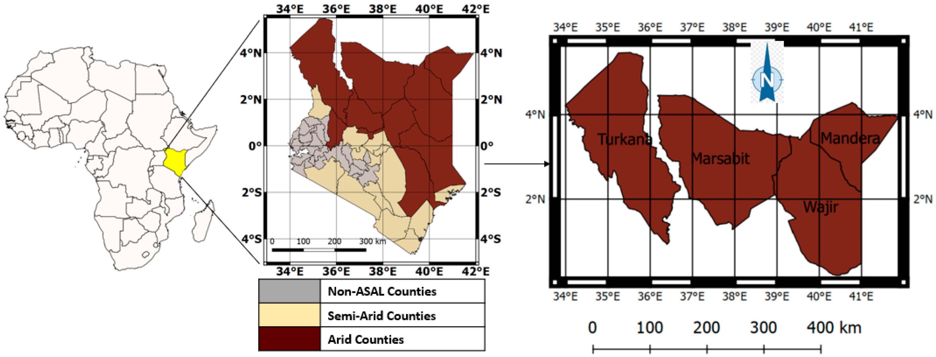
Figure 1.
The study area (to the right) and its location within Kenya. The inset (left) provides the location of Kenya in Africa while the map of Kenya (center) shows the grouping of the 47 Kenyan counties into arid and semi-arid lands (ASAL) and non-ASAL.
Figure 1.
The study area (to the right) and its location within Kenya. The inset (left) provides the location of Kenya in Africa while the map of Kenya (center) shows the grouping of the 47 Kenyan counties into arid and semi-arid lands (ASAL) and non-ASAL.
Figure 2.
Model building process from model over-production to model selection for ensemble membership. The actual model building process using both ANN and SVR are preceded by a model space reduction process undertaken by two distinct steps. First, the formulation of assumptions and second, the use of cut-off criteria on models considered predictive enough to be included in the ensembles. Not included in this scheme is the fact that all variables were normalized prior to modeling to ensure the input variables were all at a comparable range.
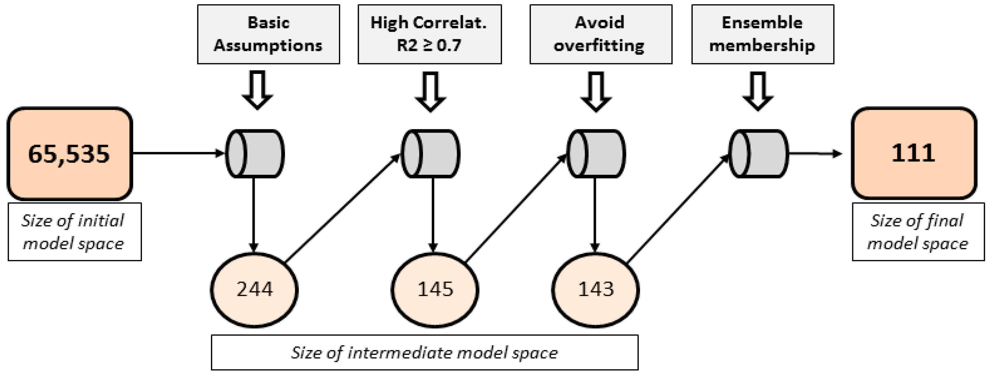
Figure 3.
Illustration of the model space reduction process. The assumption of including only one variable of a type (precipitation, vegetation and water balance) reduces the set of possible models from 65,535 to 244. The selection of models with higher performance (R2 ≥ 0.7) and the subsequent elimination of overfit models further reduces the model space to 143 models. The set of 143 models is subjected to the ensemble membership selection process using a greedy version of iterative elimination of models from the ensemble as long as no significant loss in performance is recorded. In this way, a final model space with 111 models is achieved.
Figure 4.
Sampling approach for model building (training and validation) and model testing. Only data from 2001 to 2015 was used for model building. Models were only tested using data from 2016–2017. The in-sample was randomly split (70:30) for model building and validation.
Figure 4.
Sampling approach for model building (training and validation) and model testing. Only data from 2001 to 2015 was used for model building. Models were only tested using data from 2016–2017. The in-sample was randomly split (70:30) for model building and validation.
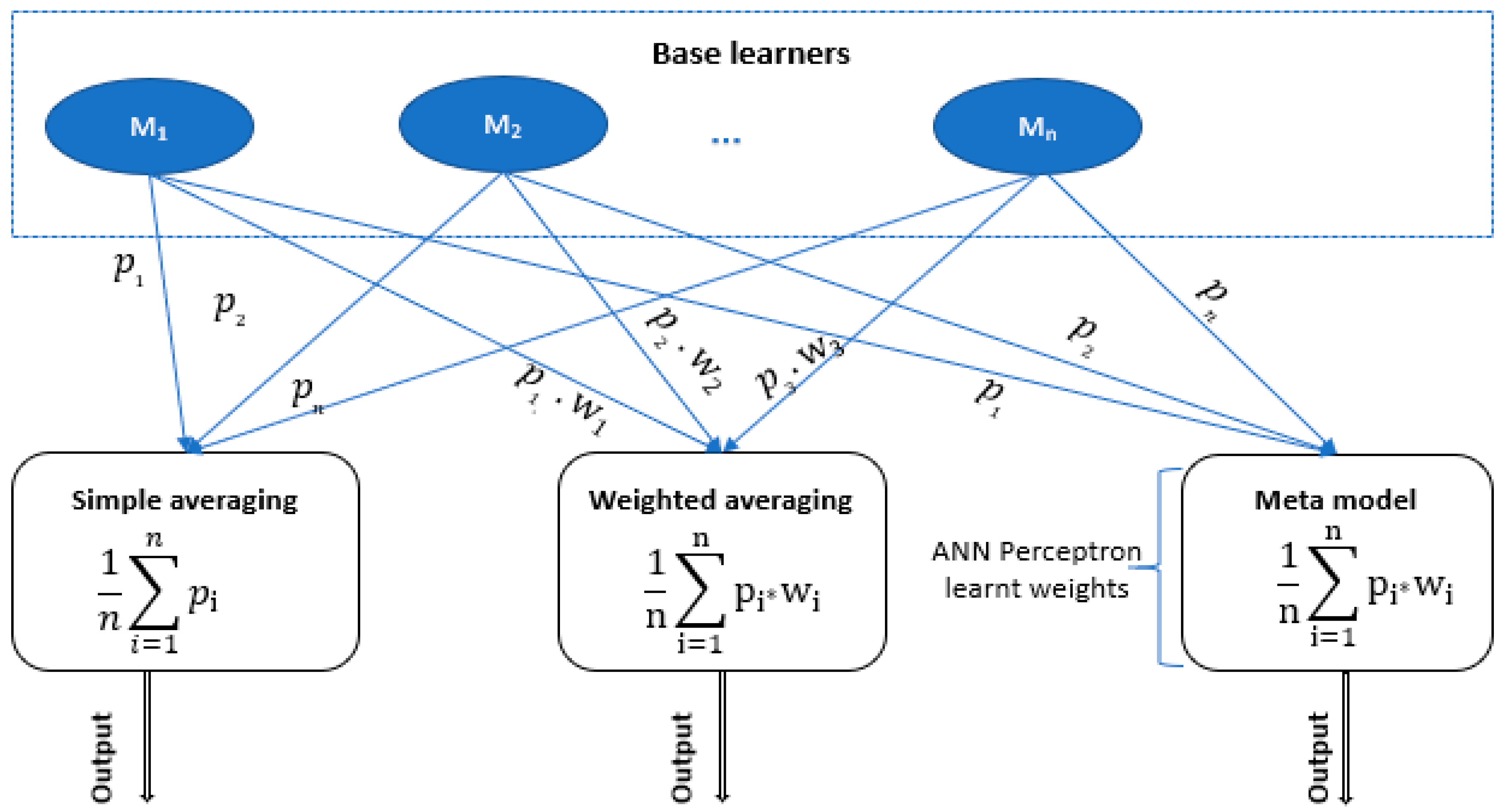
Figure 5.
Schema of the model ensemble approaches for simple averaging (left), weighted averaging (center) and model stacking (right). In the simple averaging approach, the models have equal weights and so the model outputs are non-weighted. In the weighted averaging approach, the performance of the models in the validation dataset is used to assign weights to the model. The model stacking approach uses the outputs of the individual models as inputs to a meta model (ANN perceptron) that is then used to tune weights assigned to the individual models.
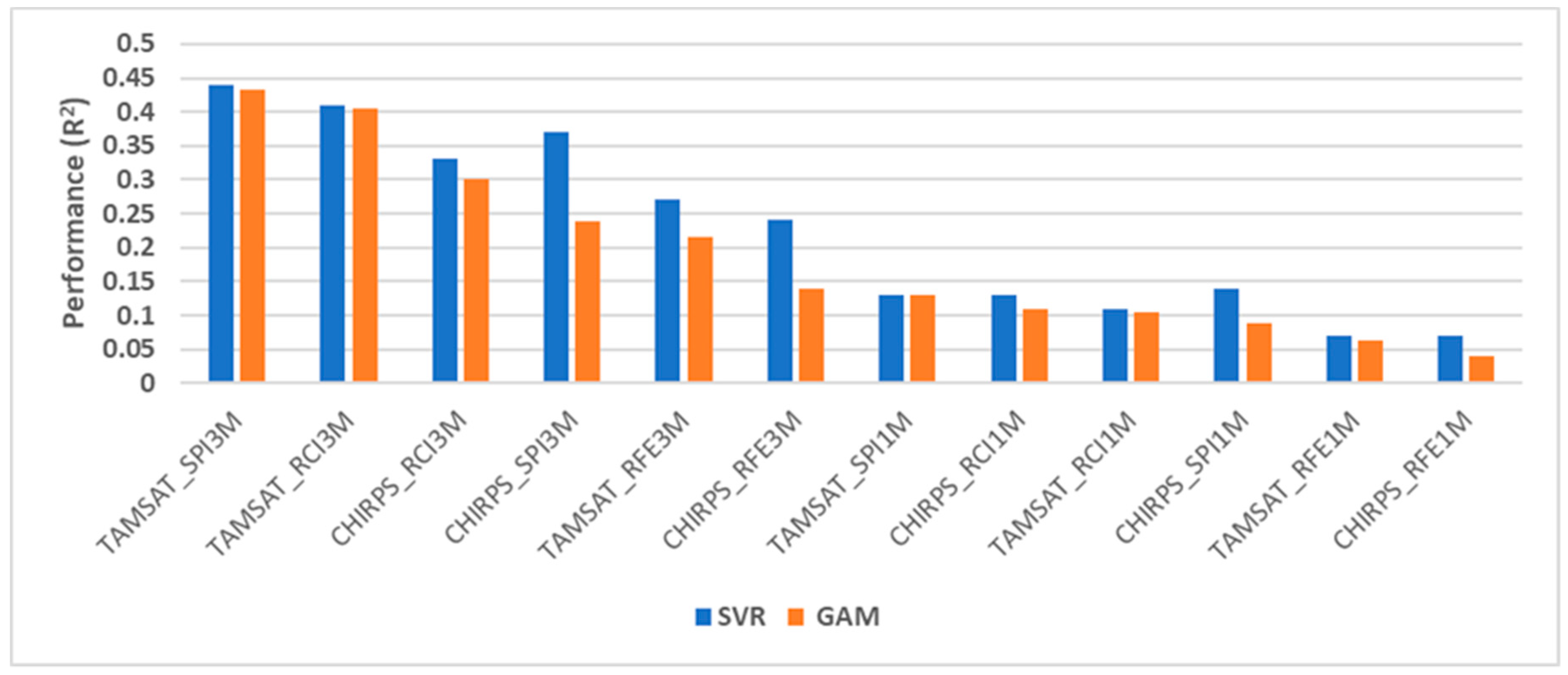
Figure 6.
R2 for SVR and GAM models for variable selection. The presented R2 is between drought severity (VCI3M) and the precipitation variables of either TAMSAT or CHIRPS. The single variable models were developed with the same configurations using the in-sample datasets covering the period 2001–2015.
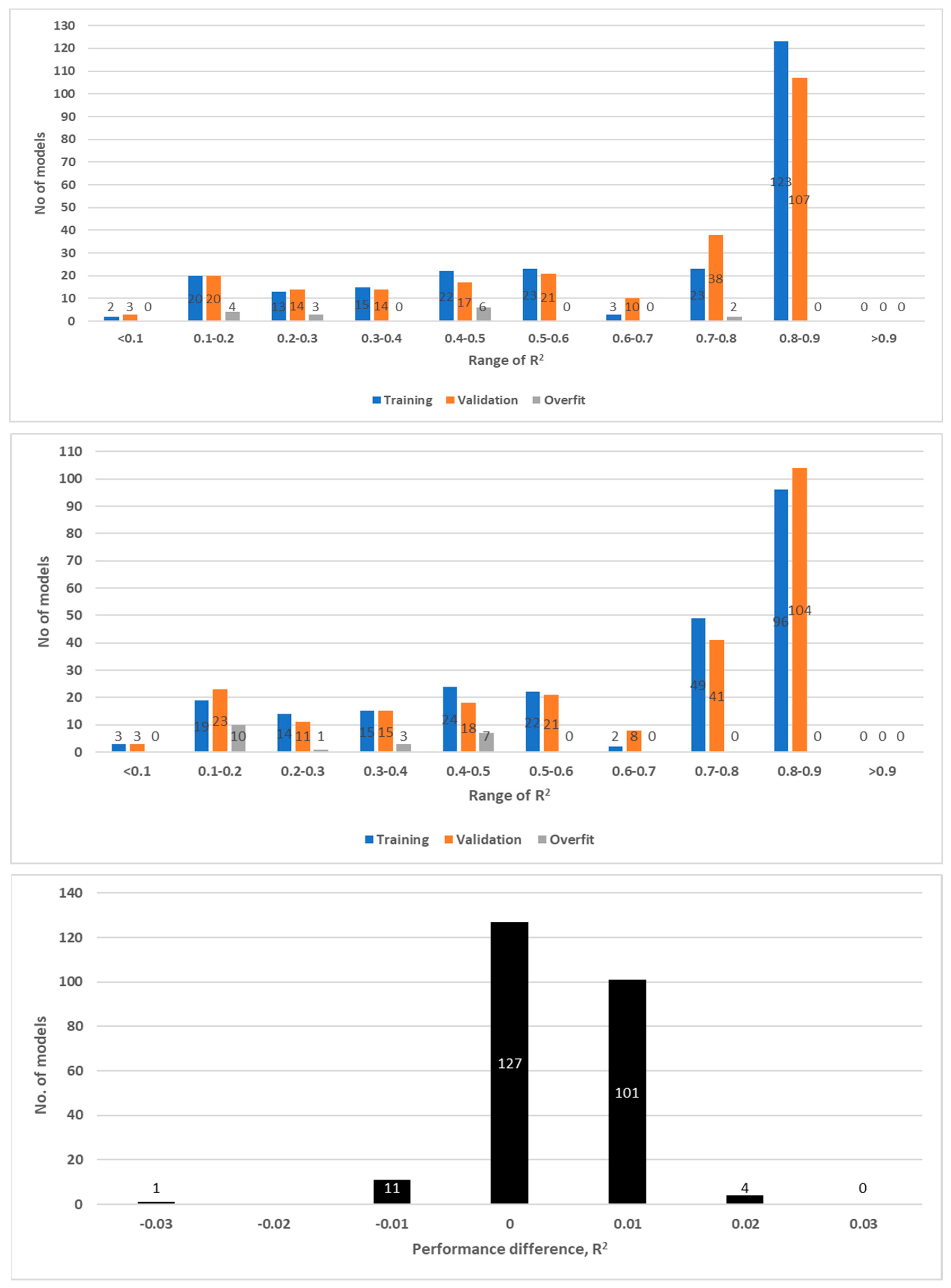
Figure 7.
Performance of ANN (
top) and SVR models (
center) in the prediction of VCI3M grouped by performance (R
2). Models indicating significant overfitting problems are highlighted in gray. The model training uses the in-sample data (2001–2015) and follows on training with 70% and validating on 30% of the data as described in
Section 2.7.3 on sample selection. (
bottom) Performance difference between ANN and SVR model pairings in the validation dataset. The performance of the ANN and SVR models are rounded off to two decimal places prior to the calculation of the performance difference. The zero (0) difference represents 127 cases for which the SVR model equals the ANN models in performance. To the left of zero difference are the cases (12) in which SVR models outperform ANN models while to the right are cases (105) for which ANN models are superior to SVR models.
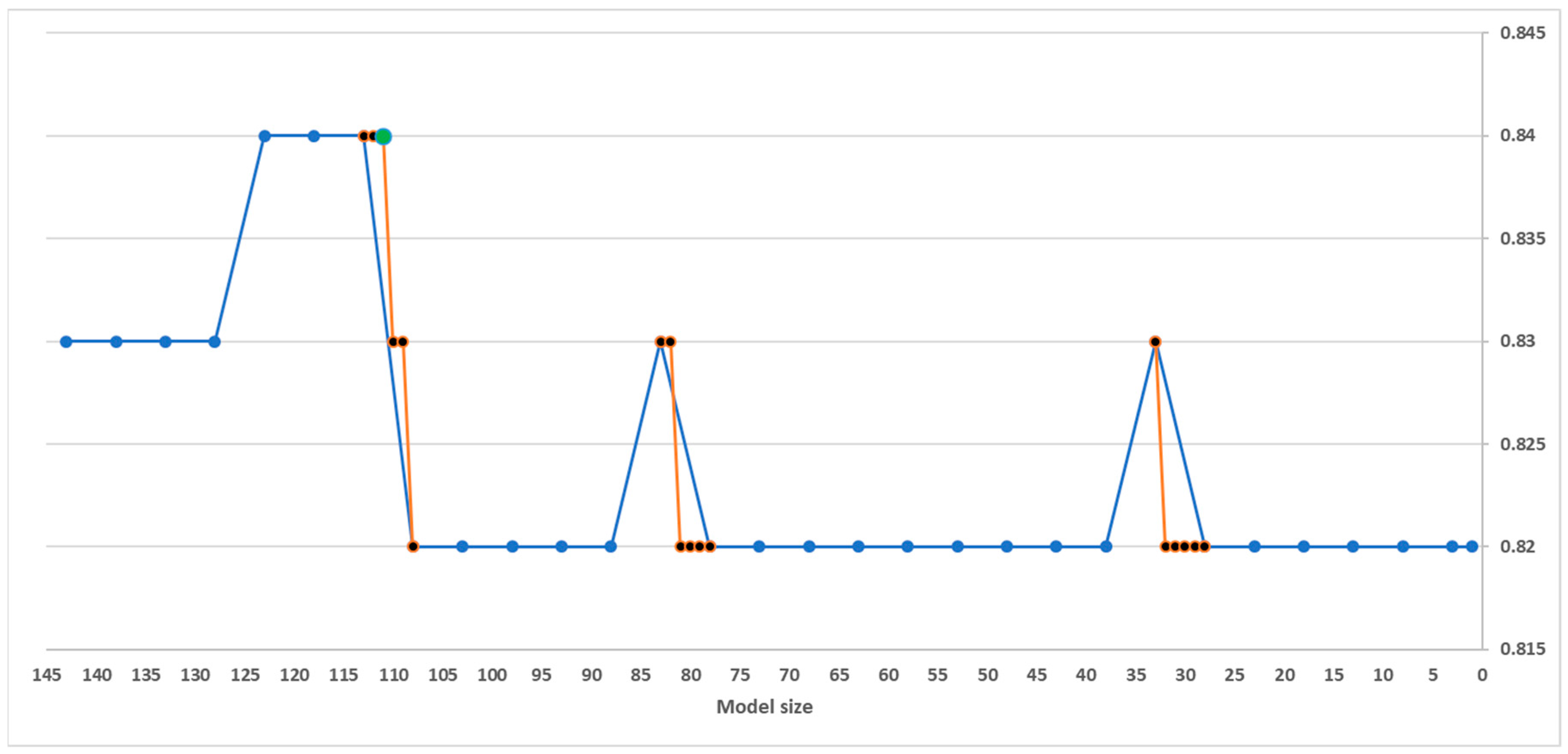
Figure 8.
Ensemble membership selection showing the reduction from 143 models to 111 models (green dot) in the ensemble using the back-forward selection procedure. The models are eliminated in batches of five (blue lines) but in instances where a drop of performance is realized, a forward selection beginning with the last smallest ensemble size is done by the addition of one model at a time (orange lines in the plot). The values are rounded off to maximum two digits.
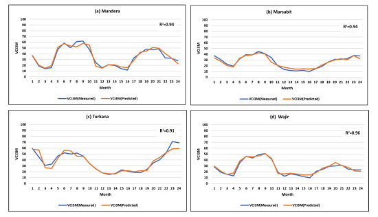
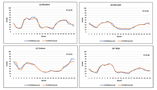
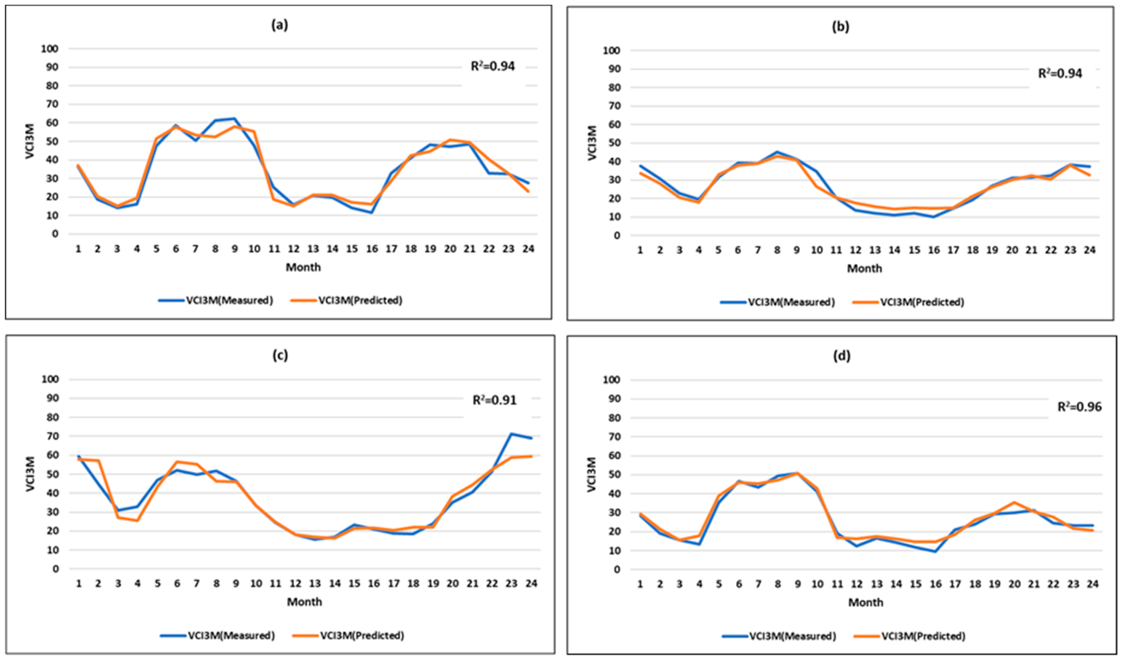
Figure 9.
Plot of the actual values of VCI3M versus the values predicted 1 month ahead from the heterogeneous stacked ensembles in the test data over 24 months for (a) Mandera (R2 = 0.94); (b) Marsabit (R2 = 0.94); (c) Turkana (R2 = 0.91) and (d) Wajir (R2 = 0.96). Results are for out-of-sample data (2016–2017).
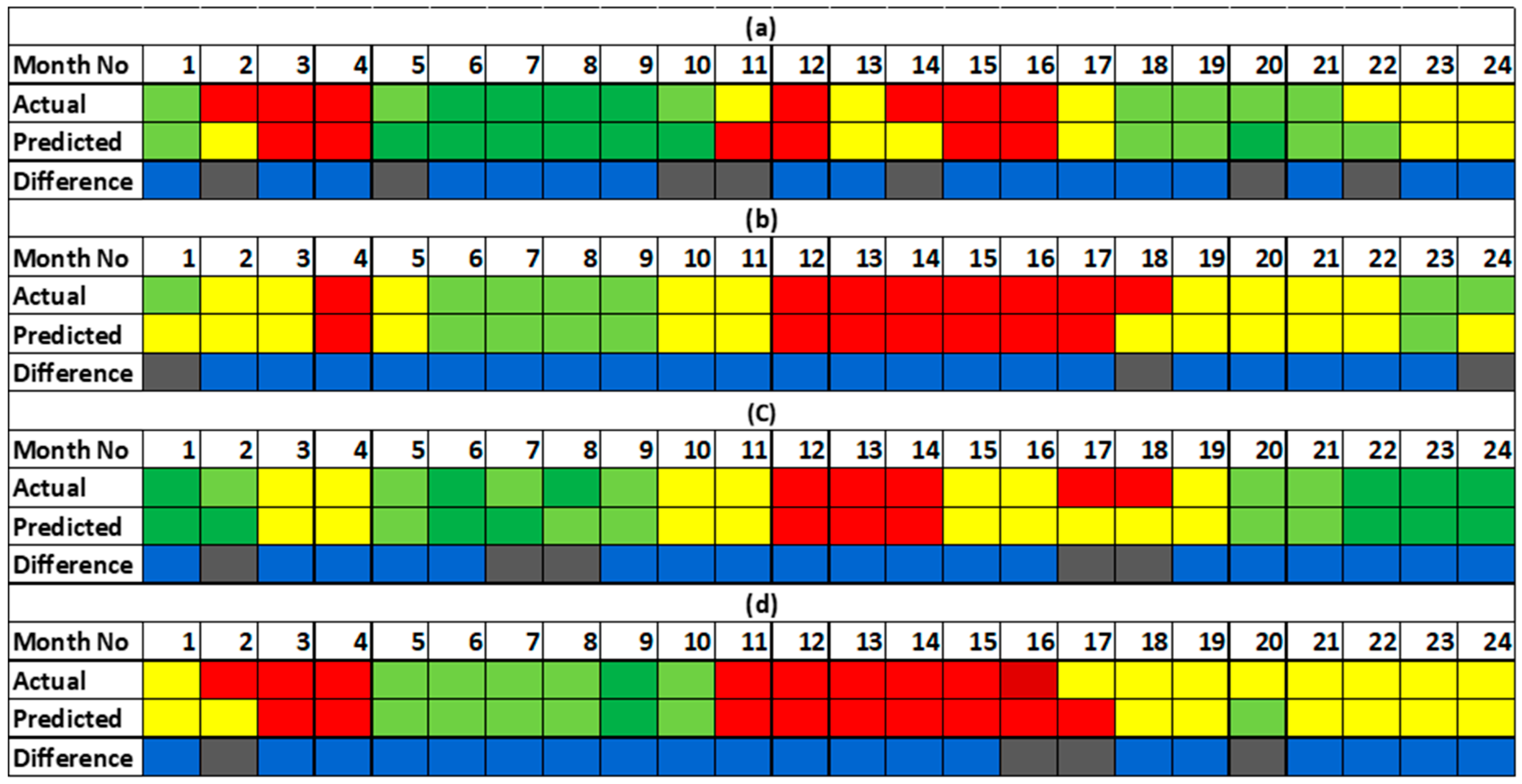
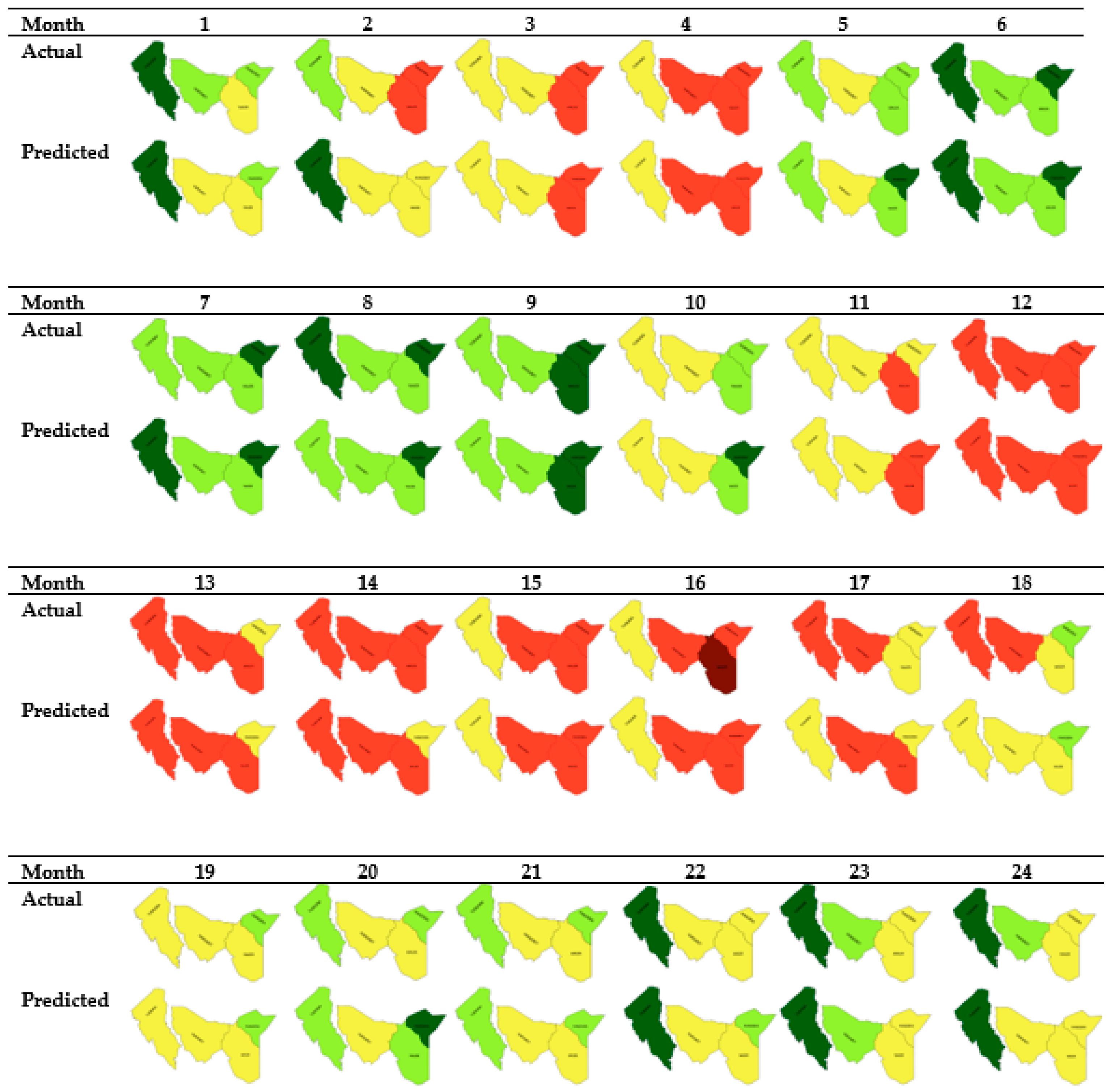
Figure 10.
Performance of the heterogeneous stacked ensemble classifier for the each of the counties showing months of difference in grey and those of agreement in blue. Predictions were made 1 month ahead. The classification accuracies are: (a) 71% for Mandera county; (b) 88% for Marsabit county; (c) 79% for Turkana county and; (d) 83% for Wajir county.
Table 1.
The study base datasets: categories, sources and description. The sources are grouped into three classes: (1) precipitation-related indices, (2) vegetation-related indices, and (3) water balance indices.
Table 1.
The study base datasets: categories, sources and description. The sources are grouped into three classes: (1) precipitation-related indices, (2) vegetation-related indices, and (3) water balance indices.
| Base Dataset | Source | Description |
|---|
| Vegetation |
| Normalized Difference Vegetation Index (NDVI) | LPDAAC Didan [36,37] | Combination of both MODIS Terra (MOD13Q1) & MODIS Aqua (MCD13Q1) using the Whittaker smoothing approach [9] |
| Precipitation |
| Rainfall Estimates (RFE) | RFE from both TAMSAT [38] and CHIRPS [39] | TAMSAT version 3.0 product & CHIRPS version 2.0 product aggregated and spatially sub-set by BOKU |
| Water Balance |
| Land Surface Temperature data (LST) | LPDAAC [40] | MODIS Terra Land Surface Temperature/Emissivity 8-Day L3 Global 1km SIN Grid V006 product (MOD11A2) |
| Evapotranspiration (EVT) | LPDAAC [41] | MODIS/Terra Net Evapotranspiration 8-Day L4 Global 500 m SIN Grid V006 (MOD16A2). |
| Potential Evapotranspiration (PET) | LPDAAC [41] | MODIS/Terra Net Evapotranspiration 8-Day L4 Global 500 m SIN Grid V006 (MOD16A2) |
| Standardized Precipitation-Evapotranspiration (SPEI) | SPEI Global Drought Monitor [42] | The standardized difference between precipitation and potential evapotranspiration [43]. |
Table 2.
Variables used in the study to predict vegetation condition index (VCI). Near infrared (NIR) and Red are the spectral reflectances in near infrared and red spectral channels of MODIS satellite.
Table 2.
Variables used in the study to predict vegetation condition index (VCI). Near infrared (NIR) and Red are the spectral reflectances in near infrared and red spectral channels of MODIS satellite.
| No | Variable | Variable Description | Index Calculation |
|---|
| 1 | NDVIdekad | NDVI for last dekad of the month | NDVI = (NIR-Red)/(NIR + Red) |
| 2 | VCIdekad | VCI for the last dekad of the month | Transformed NDVI based on Equation (1) |
| 3 | VCI1M | VCI aggregated over 1 month | Transformed NDVI based on Equation (1) |
| 4 | VCI3M | VCI aggregated over the last 3 months | Transformed NDVI based on Equation (1) |
| 5 | TAMSAT_RFE1M | TAMSAT RFE aggregated over 1 month | TAMSAT RFE version 3 product (in mm) [38] |
| 6 | TAMSAT_RFE3M | TAMSAT RFE aggregated over the last 3 months | TAMSAT RFE version 3 product (in mm) [38] |
| 7 | TAMSAT_RCI1M | TAMSAT Rainfall Condition Index (RCI) aggregated over the last 3 months | TAMSAT RFE based on Equation (1) |
| 8 | TAMSAT_RCI3M | TAMSAT RCI aggregated over the last 3 months | TAMSAT RFE based on Equation (1) |
| 9 | TAMSAT_SPI1M | TAMSAT Standardized Precipitation Index (SPI) aggregated over the last 1 month | TAMSAT RFE transformed to a normal distribution so that SPImean c,i = 0 [44]. |
| 10 | TAMSAT_SPI3M | TAMSAT SPI aggregated over the last 3 months | TAMSAT RFE transformed to a normal distribution so that SPImean c,i = 0 [44] |
| 11 | CHIRPS_RFE1M | CHIRPS RFE aggregated over 1 month | CHIRPS RFE version 3 product (in mm) [39]. |
| 12 | CHIRPS_RFE3M | CHIRPS RFE aggregated over the last 3 months | CHIRPS RFE version 3 product (in mm) [39]. |
| 13 | CHIRPS_RCI1M | CHIRPS RCI aggregated over the last 1 month | CHIRPS RFE based on Equation (1) |
| 14 | CHIRPS_RCI3M | CHIRPS RCI aggregated over the last 3 months | CHIRPS RFE based on Equation (1) |
| 15 | CHIRPS_SPI1M | CHIRPS SPI aggregated over the last 1 month | CHIRPS RFE transformed to a normal distribution so that SPImean c,i = 0 [44]. |
| 16 | CHIRPS_SPI3M | CHIRPS SPI aggregated over the last 3 months | Same as Index No. 15 |
| 17 | LST1M | LST aggregated over 1 month | Average LST over the last one month |
| 18 | EVT1M | EVT aggregated over 1 month | Average MODIS EVT over the last month |
| 19 | PET1M | PET aggregated over 1 month | Average MODIS PET over the last month |
| 20 | TCI1M | Temperature Condition Index (TCI) aggregated over 1 month | MODIS LST based on Equation (1) |
| 21 | SPEI1M | Standardized Precipitation Evapotranspiration Index (SPEI) aggregated over 1 month | Follows the standardization approach on the difference between precipitation (Pi) and potential evapotranspiration (PETi) using the logistic probability distribution |
| 22 | SPEI3M | SPEI aggregated over the last 3 months | Same as Index No. 21 |
Table 3.
Drought classes used to assess the performance in classification. The drought classes quantify the vegetation deficit as described in Klisch & Atzberger [
9], Adede et al. [
17], Klisch et al. [
55], and in Meroni et al. [
56]. VCI3M is the 3-monthly Vegetation Condition Index (VCI) from filtered and gap-filled MODIS NDVI data.
| VCI3M | VCI3M | Description of Class | Drought Class |
|---|
| Limit Lower | Limit Upper |
|---|
| ≤0 | <10 | Extreme vegetation deficit | 1 |
| 10 | <20 | Severe vegetation deficit | 2 |
| 20 | <35 | Moderate vegetation deficit | 3 |
| 35 | <50 | Normal vegetation conditions | 4 |
| 50 | ≥100 | Above normal vegetation conditions | 5 |
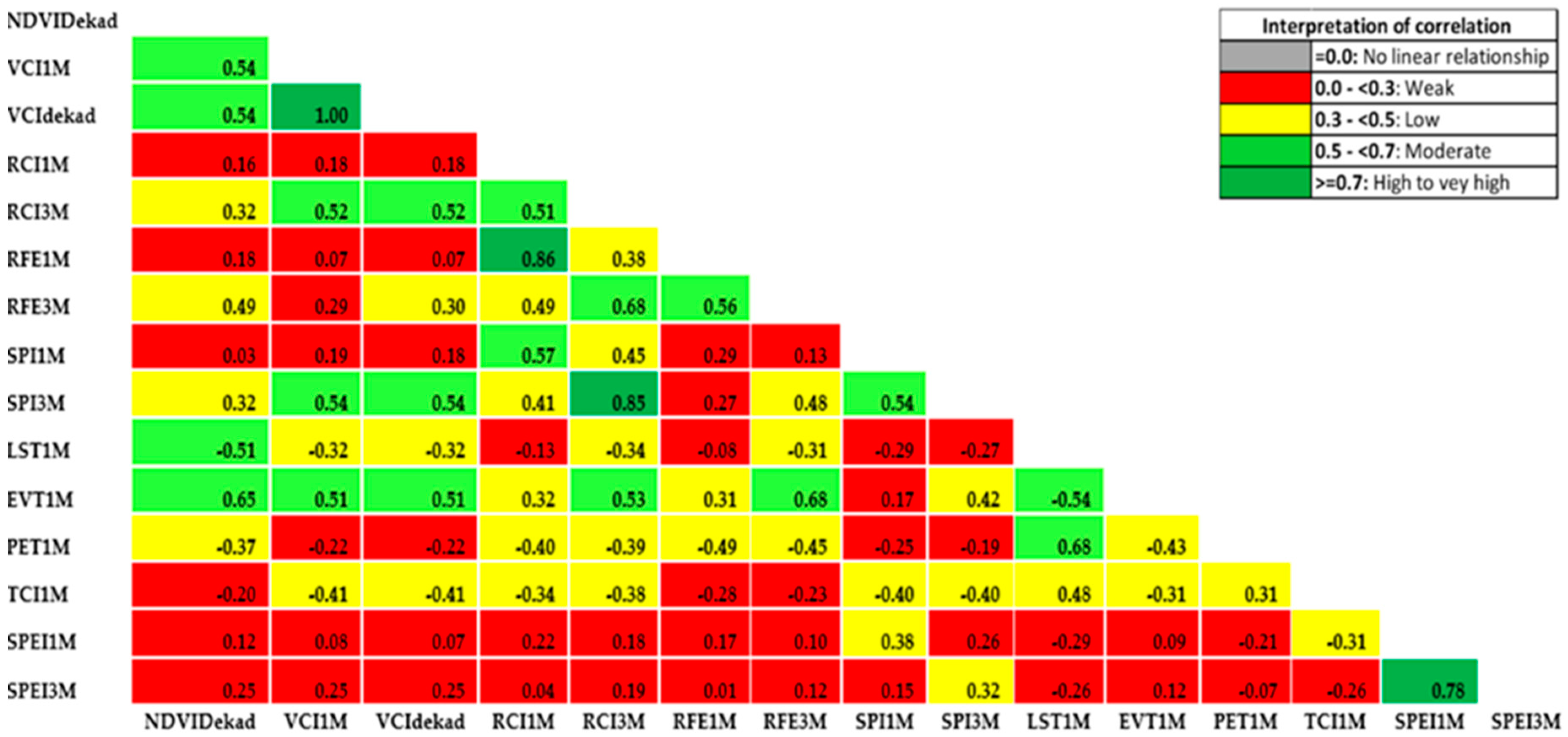
Table 4.
Spearman’s correlation of VCI3M against 1-month lag of TAMSAT/CHIRPS rainfall indicators. In bold, the higher value for each comparison.
Table 4.
Spearman’s correlation of VCI3M against 1-month lag of TAMSAT/CHIRPS rainfall indicators. In bold, the higher value for each comparison.
| Data Set | RFE1M | RFE3M | RCI1M | RCI3M | SPI1M | SPI3M |
|---|
| TAMSAT | 0.23 | 0.39 | 0.33 | 0.64 | 0.38 | 0.64 |
| CHIPRS | 0.10 | 0.26 | 0.34 | 0.53 | 0.34 | 0.52 |
Table 5.
Correlation between the lagged predictor variables and future vegetation conditions (VCI3M). The precipitation variables are those derived from TAMSAT.
Table 5.
Correlation between the lagged predictor variables and future vegetation conditions (VCI3M). The precipitation variables are those derived from TAMSAT.
| Lagged Variable | Correlation with Drought Severity (VCI3M) |
|---|
| TCI1M_lag1 | −0.58 |
| LST1M_lag1 | −0.45 |
| PET1M_lag1 | −0.34 |
| NDVIDekad_lag1 | 0.16 |
| SPEI1M_lag1 | 0.19 |
| RFE1M_lag1 | 0.23 |
| SPEI3M_lag1 | 0.28 |
| RCI1M_lag1 | 0.33 |
| SPI1M_lag1 | 0.38 |
| RFE3M_lag1 | 0.39 |
| EVT1M_lag1 | 0.59 |
| RCI3M_lag1 | 0.64 |
| SPI3M_lag1 | 0.64 |
| VCI3M_lag1 | 0.82 |
| VCI1M_lag1 | 0.88 |
| VCIdekad_lag1 | 0.89 |
Table 6.
Performance (R2) of the champion models for each of the counties in the study area on the out-of-sample dataset covering the period 2016–2017. Note that the models are non-county specific. Also reported is the overall performance across all four counties.
Table 6.
Performance (R2) of the champion models for each of the counties in the study area on the out-of-sample dataset covering the period 2016–2017. Note that the models are non-county specific. Also reported is the overall performance across all four counties.
| Mandera | Marsabit | Turkana | Wajir | Overall |
|---|
| ANN | 0.79 | 0.79 | 0.86 | 0.79 | 0.82 |
| SVR | 0.70 | 0.77 | 0.88 | 0.71 | 0.78 |
Table 7.
Performance (R2) of the ANN homogeneous model ensembles for each county. Each approach has the results derived from the non-weighted, weighted and stacked approaches of model ensembling. For comparison, the ANN champion model is also included (top row). In bold, the best results.
Table 7.
Performance (R2) of the ANN homogeneous model ensembles for each county. Each approach has the results derived from the non-weighted, weighted and stacked approaches of model ensembling. For comparison, the ANN champion model is also included (top row). In bold, the best results.
| Approach | Mandera | Marsabit | Turkana | Wajir | Overall |
|---|
| ANN Champion | 0.79 | 0.79 | 0.86 | 0.79 | 0.82 |
| ANN Homogeneous Simple Average | 0.78 | 0.86 | 0.88 | 0.80 | 0.84 |
| ANN Homogeneous Weighted Average | 0.79 | 0.86 | 0.88 | 0.81 | 0.85 |
| ANN Homogeneous Stacked | 0.93 | 0.87 | 0.89 | 0.93 | 0.91 |
Table 8.
Performance (R2) of the SVR homogeneous model ensembles for each county. Each approach has the results derived from the non-weighted, weighted and stacked approaches of model ensembling. For comparison, the SVR champion model is also included (top row). In bold, the best results.
Table 8.
Performance (R2) of the SVR homogeneous model ensembles for each county. Each approach has the results derived from the non-weighted, weighted and stacked approaches of model ensembling. For comparison, the SVR champion model is also included (top row). In bold, the best results.
| Approach | Mandera | Marsabit | Turkana | Wajir | Overall |
|---|
| SVR Champion | 0.70 | 0.77 | 0.88 | 0.71 | 0.78 |
| SVR Homogeneous Simple Average | 0.71 | 0.80 | 0.87 | 0.73 | 0.80 |
| SVR Homogeneous Weighted Average | 0.71 | 0.80 | 0.87 | 0.73 | 0.80 |
| SVR Homogeneous Stacked | 0.88 | 0.85 | 0.88 | 0.88 | 0.88 |
Table 9.
Classification accuracy for the ANN homogeneous ensembles. Each approach has the results derived from the non-weighted, weighted and stacked approaches of model ensembling. For comparison, the ANN champion model is also included (top row). In bold, the best results.
Table 9.
Classification accuracy for the ANN homogeneous ensembles. Each approach has the results derived from the non-weighted, weighted and stacked approaches of model ensembling. For comparison, the ANN champion model is also included (top row). In bold, the best results.
| Approach | Mandera | Marsabit | Turkana | Wajir | Overall |
|---|
| ANN Champion | 0.71 | 0.75 | 0.71 | 0.67 | 0.71 |
| ANN Homogeneous Simple Average | 0.67 | 0.83 | 0.67 | 0.63 | 0.70 |
| ANN Homogeneous Weighted Average | 0.67 | 0.79 | 0.67 | 0.63 | 0.69 |
| ANN Homogeneous Stacked | 0.79 | 0.88 | 0.75 | 0.71 | 0.78 |
Table 10.
Classification accuracy for the SVR homogeneous ensembles. Each approach has the results derived from the non-weighted, weighted and stacked approaches of model ensembling. For comparison, the SVR champion model is also included (top row). In bold, the best results.
Table 10.
Classification accuracy for the SVR homogeneous ensembles. Each approach has the results derived from the non-weighted, weighted and stacked approaches of model ensembling. For comparison, the SVR champion model is also included (top row). In bold, the best results.
| Approach | Mandera | Marsabit | Turkana | Wajir | Overall |
|---|
| SVR Champion | 0.58 | 0.75 | 0.83 | 0.58 | 0.69 |
| ANN Homogeneous Simple Average | 0.63 | 0.83 | 0.67 | 0.63 | 0.69 |
| ANN Homogeneous Weighted Average | 0.63 | 0.83 | 0.71 | 0.63 | 0.70 |
| ANN Homogeneous Stacked | 0.79 | 0.88 | 0.75 | 0.71 | 0.78 |
Table 11.
Performance (R2) of the heterogeneous model ensembles for each county. Each approach has the results derived from the non-weighted, weighted and stacked approaches to model ensembling. For comparison, the ANN and SVR champion models are also included. In bold, the best results.
Table 11.
Performance (R2) of the heterogeneous model ensembles for each county. Each approach has the results derived from the non-weighted, weighted and stacked approaches to model ensembling. For comparison, the ANN and SVR champion models are also included. In bold, the best results.
| Approach | Mandera | Marsabit | Turkana | Wajir | Overall |
|---|
| ANN Champion | 0.79 | 0.79 | 0.86 | 0.79 | 0.82 |
| SVR Champion | 0.70 | 0.77 | 0.88 | 0.71 | 0.78 |
| Heterogeneous Simple Average | 0.74 | 0.82 | 0.87 | 0.76 | 0.82 |
| Heterogeneous Weighted Average | 0.76 | 0.83 | 0.88 | 0.78 | 0.82 |
| Heterogeneous Stacked | 0.94 | 0.94 | 0.91 | 0.96 | 0.94 |
Table 12.
Classification accuracy of the heterogeneous ensemble. Each approach has the results derived from the non-weighted, weighted and stacked approaches to model ensembling. For comparison, the ANN and SVR champion models are also included. In bold, the best results.
Table 12.
Classification accuracy of the heterogeneous ensemble. Each approach has the results derived from the non-weighted, weighted and stacked approaches to model ensembling. For comparison, the ANN and SVR champion models are also included. In bold, the best results.
| Approach | Mandera | Marsabit | Turkana | Wajir | Overall |
|---|
| ANN Champion | 71 | 75 | 71 | 67 | 71 |
| SVR Champion | 58 | 75 | 83 | 58 | 69 |
| Heterogeneous Simple Average | 63 | 83 | 71 | 63 | 70 |
| Heterogeneous Weighted Average | 63 | 83 | 71 | 67 | 71 |
| Heterogeneous Stacked | 71 | 88 | 79 | 83 | 80 |
Table 13.
Performance in the prediction of moderate to extreme droughts using the heterogeneous stacked ensemble compared to the best ANN and SVR models. In bold, the best results.
Table 13.
Performance in the prediction of moderate to extreme droughts using the heterogeneous stacked ensemble compared to the best ANN and SVR models. In bold, the best results.
| County | ANN Champion | SVR Champion | Heterogeneous
Stacked Ensemble |
|---|
| Mandera | 0.62 | 0.46 | 0.69 |
| Marsabit | 0.71 | 0.71 | 0.94 |
| Turkana | 0.75 | 0.00 | 0.83 |
| Wajir | 0.72 | 0.61 | 0.78 |
| Overall | 0.70 | 0.69 | 0.82 |


