Predicting Future Locations of Moving Objects by Recurrent Mixture Density Network

Institute of Geospatial Information, Information Engineering University, Zhengzhou 450000, China
*
Author to whom correspondence should be addressed.
ISPRS Int. J. Geo-Inf. 2020, 9(2), 116; https://0-doi-org.brum.beds.ac.uk/10.3390/ijgi9020116
Submission received: 7 January 2020
/
Revised: 8 February 2020
/
Accepted: 19 February 2020
/
Published: 20 February 2020
Abstract
:Accurate and timely location prediction of moving objects is crucial for intelligent transportation systems and traffic management. In recent years, ubiquitous location acquisition technologies have provided the opportunity for mining knowledge from trajectories, making location prediction and real-time decisions more feasible. Previous location prediction methods have mostly developed on the basis of shallow models whereas shallow models are not competent for some tricky challenges such as multi-time-step location coordinates prediction. Motivated by the current study status, we are dedicated to a deep-learning-based approach to predict the coordinates of several future locations of moving objects based on recent trajectory records. The method of this work consists of three successive parts: trajectory preprocessing, prediction model construction, and post-processing. In this work, a prediction model named the bidirectional recurrent mixture density network (BiRMDN) was constructed by integrating the long short-term memory (LSTM) and mixture density network (MDN) together. This model has the ability to learn long-term contextual information from recent trajectory and model real-valued location coordinates. We employed a vessel trajectory dataset for the implementation of this approach and determined the optimal model configuration after several parameter analysis experiments. Experimental results involving a performance comparison with other widely used methods demonstrate the superiority of the BiRMDN model.
1. Introduction
Location prediction refers to estimating the anticipated location at several following timestamps based on recent trajectory and the current status [1]. Predicting the future location of moving objects (residents, cars, vessels, etc.) is of great importance for a wide spectrum of novel applications such as location-based recommendation services [2], intelligent transportation systems [3], maritime surveillance [4], and aviation monitoring [5], etc. (e.g., in the maritime industry, if the future locations of vessels in the upcoming period of time are known in advance, the maritime management system can assess the collision risk or detect the abnormal behavior. If there are any risks, vessels will receive alerts from the management system to change the pre-planned route). Traffic management and route plans can also be implemented based on the location prediction of vehicles. However, location prediction is a challenging issue due to the complexity and diversity of mobility behavior. Future locations in the evolution of trajectory are uncertain events affected by both the internal motivation of moving objects and the external factors. Thus, traditional approaches that rely on the kinematic equation and linear model fail to achieve a satisfactory performance, since they are limited in taking into account the inherent dynamics of moving objects.
In the past few years, navigation and positioning technology has developed rapidly. A large number of vehicles, mobile devices, and wearable devices are equipped with a location acquisition function unit. Trajectory records can be generated and collected by these prevalent vehicles and devices in real-time and a consecutive manner [6]. Ubiquitous trajectory data lead to the increasing advent of data-driven location prediction methods [7], since trajectories of moving objects result from the integrated influence of both internal motivation and external factors. Spatiotemporal information describing the mobility behavior is a valuable resource in trajectory data. We can obtain the information by trajectory mining and utilize it to predict the future location of moving objects. Trajectory mining in a data-driving manner has the prominent advantage of being easy to transplant, since it reduces the dependency on domain knowledge when accomplishing the location prediction task. The process of trajectory mining for location prediction consists of two phases: (1) the offline prediction model training by exploiting history trajectories, and (2) real-time location prediction based on the well-trained model.
There are some widely researched prediction techniques based on trajectory mining in previous studies such as content-based techniques [8], pattern-based techniques [9,10], and representation-based techniques, [11,12] etc. The Markov chain model is a typical strategy of content-based techniques, in which the next location is assumed to be dependent on the current status. It is trained by constructing a transition matrix based on history trajectories, which indicates the transition probability between locations. The next location will be inferred depending on the current status and the transition matrix [13]. Pattern-based techniques aim to mine the mobility patterns existing in history trajectories by utilizing association rule methods. Then, the mobility patterns are used to predict future locations [9].
However, the methods above-mentioned have mainly focused on the current state of moving objects and neglect the historical information contained in long-term location sequence. The absence of historical information evidently limits the prediction performance, especially in long-term prediction. Additionally, it is difficult for most of these methods that are in a discrete manner to model real-valued location coordinates. In recent years, representation-based techniques leveraging deep learning algorithms have attracted much attention. Representation-based techniques adequately learn historical information and representative features implied by trajectories. The extracted features are beneficial to the improvement of prediction accuracy [11]. Nevertheless, there are still some bottlenecks that exist in the current representation-based methods. It is tricky for deep learning algorithms such as the recurrent neural network (RNN) [14] and convolutional neural network (CNN) [15], which are good at performing discrete prediction, to predict real-valued location coordinates. The existing prediction methods will be confused by the continuous and non-repetitive target. The prediction goals of some studies are discrete targets such as spatial cells or significant places [16] and a spatial discretization strategy or clustering processing is introduced to transform the continuous real-valued coordinates into discrete targets, which also may lead to the sparsity issue and curse of dimensionality.
Motivated by the limitations of the existing methods in predicting long-term location coordinates, we dedicated this paper to a location prediction approach based on deep learning. The core of this approach is the construction of a bidirectional recurrent mixture density network (BiRMDN) model. BiRMDN is a deep learning model integrating a bidirectional long short-term memory (LSTM) network [17] and mixture density network (MDN) [18]. The LSTM network is a variant of a recurrent neural network which is superior in capturing long-term spatiotemporal dependency and contextual information contained in trajectories. Rather than directly outputting the exact value of the predicted coordinates, MDN generates the parameters of the mixture distribution function to model locations. In other words, we only predicted the possible range of future locations and the corresponding probability.
In general, the main superiority of BiRMDN model lies in the following: (1) It is better at improving the prediction accuracy than the traditional machine learning methods due to the utilization of long-term spatiotemporal dependency and contextual information in trajectory data. (2) Given that the evolution of the trajectory is actually an uncertain event, this kind of fuzzy prediction is competent for modeling the real-valued location coordinates. The ultimate prediction results obtained by sampling from the distributions are closer to the real mobility behavior. Furthermore, the curse of dimensionality is successfully avoided in this way. (3) The learning process is automatic and there are no sophisticated hand-crafted features involved. It is easy to transplant this model to different scenarios.
Real-world vessel trajectory data [19] collected by the automatic identification system (AIS) were employed for the implementation of the proposed approach. In the experiments, we analyzed the effect of the model parameters and performed a comparison study with other widely used methods. The remainder of this paper is organized as follows. In Section 2, previous work related to location prediction are reviewed. Section 3 elaborates the proposed methodology, especially the BiRMDN model. Section 4 presents the experimental results and the corresponding evaluation. Finally, the discussion and conclusions are presented in Section 5.
2. Related Work
Pervasive trajectory data are valuable resources for data mining and knowledge discovery. Location prediction has been widely regarded as a key issue of trajectory mining. In recent years, a number of methods have been developed to improve the efficiency and accuracy of location prediction. Most of the data-driven methods have focused on mining spatiotemporal and contextual information from trajectories. These methods can be classified into three categories: content-based methods, pattern-based methods, and representation-based methods.
Content-based methods are developed on the basis of the assumption that the next location is related to the current status. The Markov chain model is a typical strategy of content-based methods. Ashbrook et al. [20] proposed a system of predicting the movement of multiple users based on the Markov model. Significant locations extracted from the trajectory data were used to construct the Markov chain. This system was applied to both single and collaborative users. Song et al. [13] investigated two location prediction methods via the users’ Wi-Fi data: Markov-based and compression-based predictors, and found that the prediction result of the low-order Markov model was more accurate than that of the compression-based method. Additionally, Mathew et al. [21] proposed predicting human mobility on the basis of hidden Markov models (HMMs). HMMs consider location characteristics as unobserved parameters and correlates with the effect of the users’ previous action. Qiao et al. [22] developed a self-adaptive parameter selection Hidden Markov model-based trajectory prediction method called HMTP*. This method solved the state retention problem existing in most HMMs-based prediction methods and greatly improved the prediction accuracy. However, most low-order Markov models do not take into account the long-term dependency and contextual information contained in spatiotemporal sequence. The prediction performance is limited by the lack of contextual information. Furthermore, the Markov model is not suitable for the prediction of continuous coordinates due to its discrete nature.
The mobility behavior of moving objects can be described concisely as the trajectory patterns hidden in history trajectories. Pattern-based methods aim to mine the specific patterns existing in trajectories and use these patterns to predict the next movement step. Monreale et al. [9] proposed a pattern-based method named WhereNext and extracted the spatiotemporal patterns from trajectories, storing the patterns in a prefix-tree structure. Then, the next location was predicted based on the tree structure. Ying et al. [23] put forward an approach mining the geographic, temporal, and semantic knowledge from trajectories simultaneously. Online prediction can be implemented based on the similitude between the current movement and the discovered patterns. Lei et al. [24] developed a framework to capture the spatiotemporal patterns of movement behavior after extracting the regions of popularity by clustering. The discovered sequential relationships among the regions and the corresponding probabilities of time can be leveraged to predict location information. However, pattern-based methods built on regions of interest (ROIs) or discrete locations are insufficient to be faced with the sparsity issue (e.g., if the next location of current trajectory has never appeared in history trajectories, it will be difficult to be predicted by pattern-based methods).
In recent years, deep learning techniques have made a remarkable achievement in many fields. Representation-based methods leveraging deep learning techniques such as RNN are also widely studied in location prediction. Given the sequential and contextual property of trajectory data, RNN and its variants are able to learn representative features more efficiently than other deep learning algorithms. Nguyen et al. [25] proposed a sequence-to-sequence model based on LSTM to predict vessels’ trajectories including the destination and estimated arrival time. This model learned the movement tendency from the spatial grids’ sequence of recent trajectory and used it to estimate the future movement of vessels. Wu et al. [26] designed two RNN-based models that captured the long-term dependency and addressed the constraints of topological structure on trajectory modeling. In the two models, trajectories were expressed in the form of the road segments’ sequence instead of frequently used spatial grids. Liu et al. [27] extended the RNN and proposed modeling the spatiotemporal contexts of the trajectories by replacing the transition matrix in the RNN with time-specific transition matrices. They also divided the continuous spatial and temporal value into discrete bins when preprocessing the location data. Feng et al. [28] proposed an attentional recurrent network named DeepMove for human mobility prediction. DeepMove captures the complicated sequential transitions and multi-level periodicity in human mobility behavior, which is applied to the discrete location prediction scene.
The methods introduced above regard the future locations of trajectory as deterministic events and discretize the continuous location coordinates into spatial grids, clusters, or other tagged encodings. The discretization operation may lead to the curse of dimensionality and sharp boundary issues. Furthermore, these methods ignore the uncertain nature of mobility behavior. In terms of modeling uncertain events, MDN achieved excellent performance. Graves et al. [29] took full advantage of MDN to predict and synthesize handwriting. Zhao et al. [30] applied deep bidirectional LSTM and MDN to the generation of a basketball trajectory. Additionally, Xu et al. [31] developed a sequence learning model based on MDN for real-time prediction of taxi demand.
In this work, the BiRMDN integrating the LSTM network and MDN has the ability to learn the contextual information from a recent part of the trajectory and exploit the probability distribution function to model the uncertainty of future locations. Thus, it is able to provide promising prediction results.
3. Methods
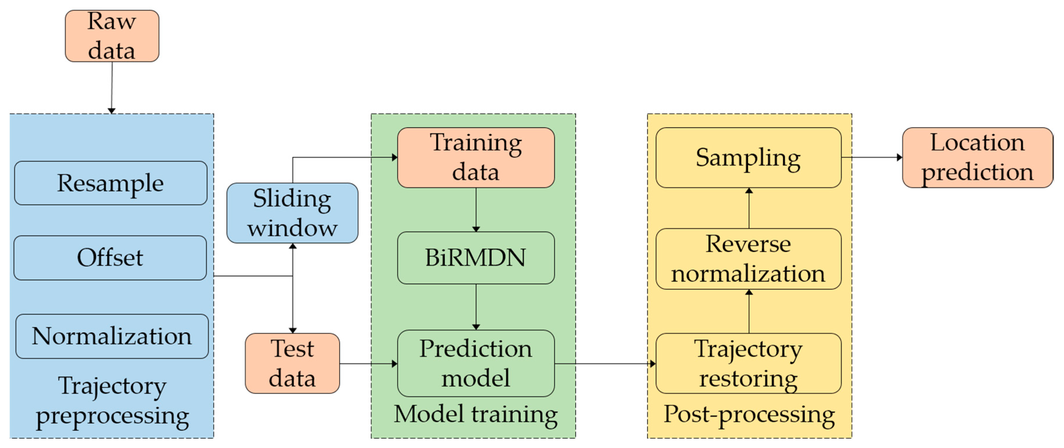
We present the location prediction methodology in this section, which contains three successive parts: (1) trajectory preprocessing; (2) construction of the BiRMDN model; and (3) post-processing to restore the trajectory. Figure 1 briefly illustrates the overall process of the proposed methodology. In the trajectory preprocessing step, instead of performing any sophisticated feature extraction, we transformed the trajectory data into normalized offset data for the BiRMDN model through only three simple steps. The well-trained BiRMDN model is capable of capturing the representative characteristics from trajectories and generating a mixed distribution of future offsets. In the stage of post-processing, the ultimate prediction results will be obtained by sampling from the generated distributions. The trajectories are restored by the reverse operation of trajectory preprocessing, which will no longer be elaborated in the following.
3.1. Problem Formulation
Definition 1.
Trajectory: Let be a set of trajectories. An individual trajectory is composed of a sequence of spatiotemporal points , where and are the origin and destination (OD) points, respectively. is the spatiotemporal point in , where (or in three-dimensional scenarios) is a location vector including the attributes of longitude and latitude, and is the corresponding timestamp.
Problem 1.
Location prediction: Given the current incomplete trajectory segment with spatiotemporal points, where the location at present time and the recent spatiotemporal points at previous timestamps are known, refer to the next locations at time instances .
In this work, a set of history trajectories were utilized to train the prediction model introduced in Section 3.3. All of the history trajectories and test trajectories were preprocessed before being fed into the model, as described in Section 3.2.
3.2. Trajectory Preprocessing
Raw positioning data were stored in the database in chronological manner. OD points were extracted to divide the consecutive positioning data into individual trajectories. The OD point extraction method is presented in our previous work [19]. Data cleaning and trajectory interpolation operations were performed to obtain usable data. According to the Problem 1 definition of location prediction, in order to unify the format of input trajectory segments and prediction results, we resampled the trajectories and adjusted the time interval between two adjacent spatiotemporal points into a fixed value.
The probability distribution function is not suitable for modeling the absolute coordinate data , which are non-stationary sequence data with tendency. Hence, we transformed the absolute coordinate sequence into the offset sequence to detrend, where is the offset from the previous location. The goal of predicting the next location is turned into predicting the offset . The concrete coordinates can be obtained by restoring the trajectory. In order to avoid the saturation issue of activation function (to be introduced in Section 3.3) occurring in the feedforward process, the input data were normalized within the range of 0 to 1 before being fed into the BiRMDN.
In the process of obtaining the training data, we utilized the sliding window method to generate the training input and the corresponding training label. As depicted in Figure 2a, we hypothesized the input sequence length , and prediction length . In the training process, the training label was delayed by time steps than the input. The sequence length of the training label was equal to that of the input. The test segment was composed of two parts: the input and ground truth, as shown in Figure 2b. In the test process, the output was also the same length as the input, but only the values at the last timestamps were picked as the prediction results.
3.3. Bidirectional Recurrent Mixture Density Network
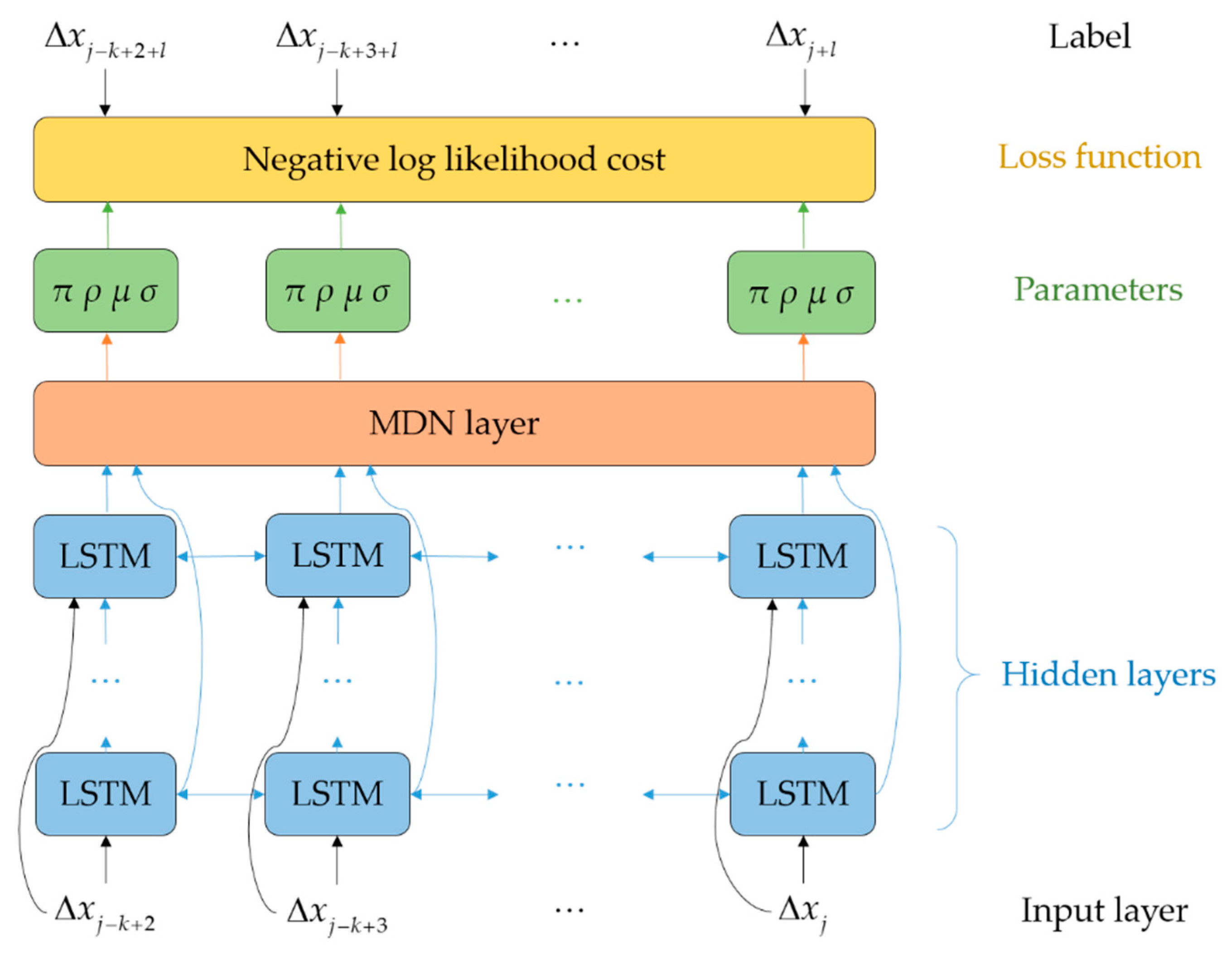
Trajectories of moving objects are chronological sequences formed by spatiotemporal points. Given the sequential characteristics of trajectory, we intuitively think of utilizing a prediction model that does well in dealing with series data. The LSTM network is a variant of RNN, which is the state-of-the-art technique in modeling series data. The most prominent character of the LSTM is the unique structure integrating the input gate, forget gate, and output gate. This structure makes it feasible for the LSTM to capture long-term spatiotemporal dependency and contextual information implied in the trajectory. Furthermore, more contextual information will be conveyed and shared if the connections among the LSTM units in the same layer of network are bidirectional [32]. However, it is tricky for an ordinary LSTM network to predict real-valued location coordinate data. Instead of outputting the coordinate results directly, the MDN outputs the parameters of the mixture probability density distribution. The mixture distribution performs well in modeling uncertain events like real-valued location data. In this work, we adopted a bidirectional connection structure in each layer of the LSTM network. Then, we added the MDN on top of the LSTM network to construct a BiRMDN for future location prediction.
Figure 3 presents the schematic of the BiRMDN model structure. The unfolded structure of the BiRMDN is composed of multiple successive layers including the input layer, hidden LSTM layers, and MDN layer. The input layer is formed by the offset sequence . The is a vector of at each timestamp . The unfolded length of the input layer is equal to , the length of the known offset sequence.
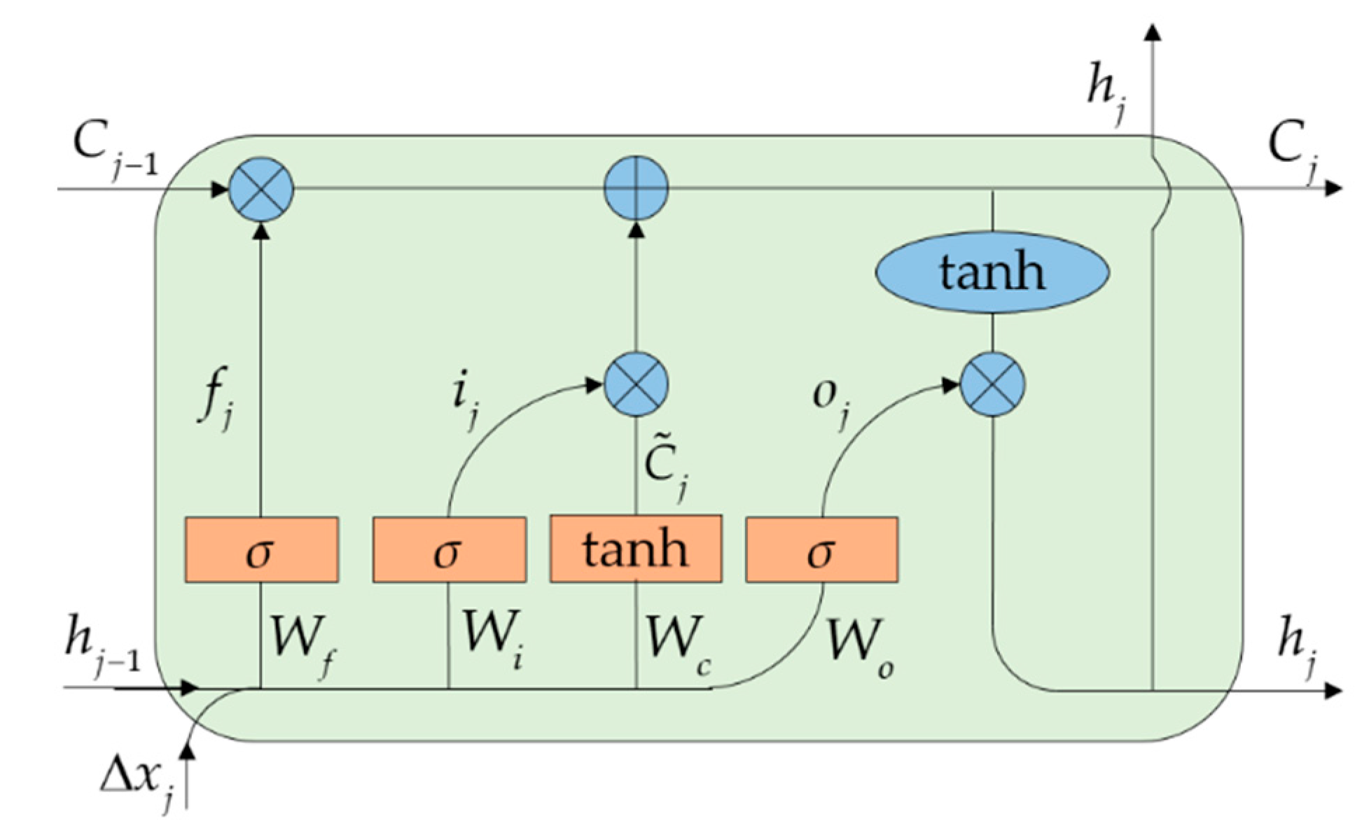
The hidden layers comprise multiple stacked LSTM layers. The input signal of each hidden layer includes both the output of the preceding layer and input layer. The LSTM layer generates an output based on the encoded input signal and its internal state. The bidirectional connection in each LSTM layer handles the sequence in both the forward and backward process through time. The output of all LSTM layers will be concatenated as the integrated output of the hidden layers. Each of the LSTM layers contains multiple connected LSTM units. The architecture of the LSTM unit is illustrated in Figure 4, which implements a hidden layer function to encode useful information based on three gates, as follows:
where , , and denote the forget gate, input gate, and output gate, respectively. and denote the logistic sigmoid function and hyperbolic tangent function, respectively, both of which are used as the nonlinear activation function. is the output of the unit in the LSTM layer. denotes the input signal from the preceding layer. The weight matrices , , and the corresponding bias associated with these gates are variables to be optimized during the training process.
The function of retaining and updating the cell state is the unique ability of the LSTM unit. is the temporary cell state, which is used to update the old cell state into new state . The state update process is determined by the cooperation of the forget gate and input gate . The weight matrices and the corresponding bias associated with the cell states are also variables to be optimized. Finally, the updated cell state is activated by the nonlinear activation function and controlled by output gate to generate output signal .
The MDN layer on top of the LSTM layers is a full-connected layer as follows:
where denotes the number of stacked LSTM layers, and and are the forward and backward output of the bidirectional LSTM layer. and denote the weight matrices connecting the bidirectional LSTM layer and the MDN layer, respectively; is the corresponding bias; and denotes the output of MDN layer. The output of the MDN layer is used to parameterize the mixture probability density distribution of the real-valued offsets. The distribution is formed by weighted components. Part of the output is used to determine the weights, while the rest is used to parameterize each individual component. In this work, we adopted the bivariate Gaussian function as the component to model the distribution of the two-dimensional offset vector . As shown in Figure 3, in addition to the weights , the parameters of the Gaussian mixture distribution includes sets of means , standard deviations , and correlations :
All parameters need to be normalized to meaningful ranges as the final output of the BiRMDN:
The normalization strategies are determined according to the Gaussian mixture distribution where:
Given the final output , the probability density function of the label is defined as follows:
where is the bivariate Gaussian function:
Loss function measuring the discrepancy between the training label and model output is defined as the negative log likelihood function:
Loss function is the objective function to be optimized during the training process by means of gradient descent. In order to avoid the issue of gradient explosion, which frequently occurs in the training process, we employed the gradient clipping strategy [33] to restrict the gradient into a predefined range. Limited by the volume of the training dataset and the complexity of the network structure, overfitting is an inevitable issue for the BiRMDN model. We adopted the dropout technique [34] to stochastically remove a portion of hidden neurons with a certain probability in each iteration. The dropout technique reduces the complexity of the network and the co-adaption of neurons. Thus, the dropout technique alleviates the overfitting issue and significantly promotes the generalization ability of the prediction model.
4. Experimental Results
In this section, we implement the location prediction method to a real-world vessel trajectory dataset and evaluate the performance. In Section 4.1, we present a brief introduction about the dataset and experimental setup. With regard to the effect of the parameters, we test the performance of the models with different parameter settings and determine the optimal configuration in Section 4.2. The comparison experiments with other widely used approaches are carried out in Section 4.3.
4.1. Dataset and Experiment Setup
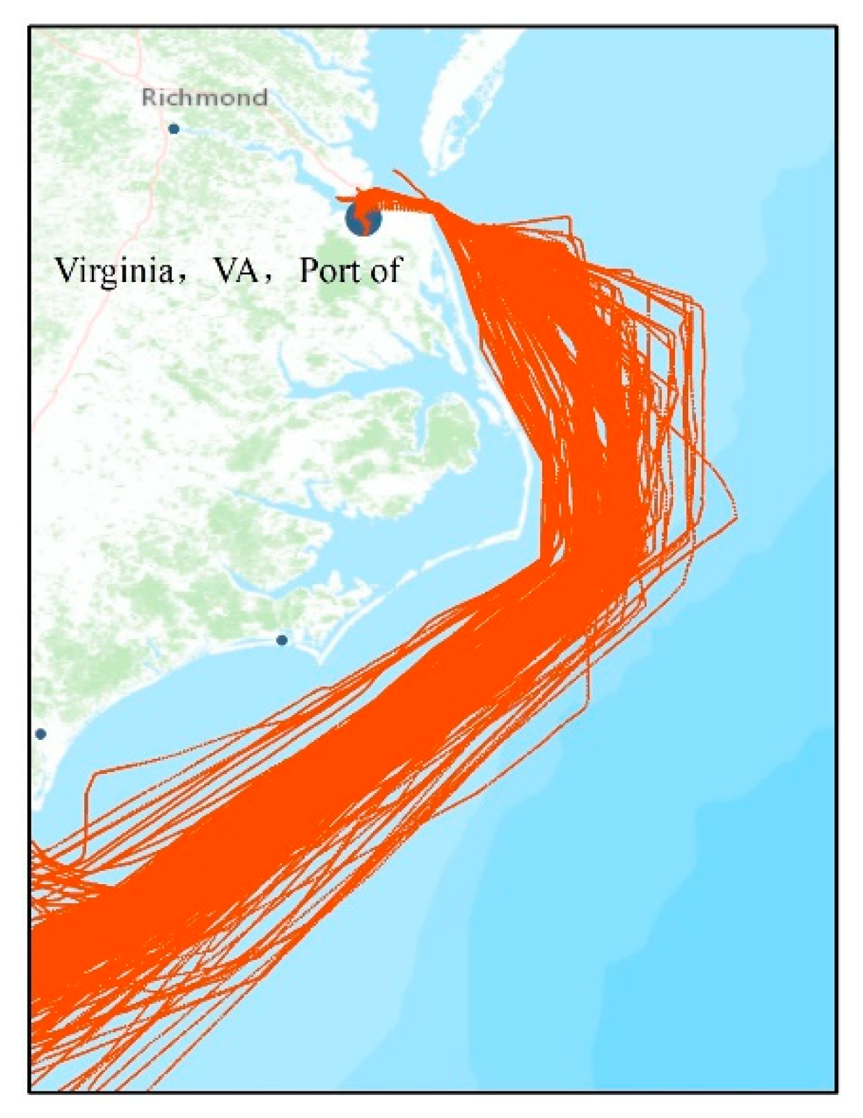
The vessel trajectory data employed for evaluation were the AIS data obtained from MarineCadastre.gov [35]. The AIS is a system equipped on large vessels that broadcasts messages to the management center at certain time frequencies. The AIS data contain static data about vessel information such as the maritime mobile service identity (MMSI), the name, and size etc., and dynamic data recording voyage information such as locations, timestamps, and speed over ground (SOG), etc. The spatiotemporal point is constituted in the attributes of dynamic data including longitude, latitude, and the corresponding timestamp. The study region is located in the eastern waters of the U.S. (from N31.8° to N37.3° and W74.3° to W78°). The dataset covers 278 completed trajectories of several types of vessels (towing, pleasure craft, tugs, and cargo ships) traveling back and forth between the Florida Strait and Port of Virginia in four consecutive months from 1 May to 31 August, 2014. In the resampling process, the fixed value of the time interval between two adjacent points was set to 10 min, according to the practical vessel sailing situation. The usable trajectories after preprocessing are delineated in Figure 5.
We used the two-hour long incomplete trajectory segment to predict the locations in the upcoming one hour (i.e., the input length of location sequence was 13 and the prediction length was six. We randomly selected 10% of the trajectories as test data and the remaining 90% as training data. After trajectory preprocessing, a total of 31,508 trajectory segments were obtained to train the prediction model.
In the process of model training, the training data were fed into the BiRMDN model in batches. One of the batches served as the validation data to determine whether the training process converges and when to terminate. We employed the adaptive moment estimation (Adam) optimizer [36] with a decayed learning rate to optimize the objective function in the back-propagation through time (BPTT) process. The dropout probability was set to 0.2 to cope with the overfitting issue.
The location coordinates are represented by longitude and latitude. We employed two performance metrics to evaluate the prediction effectiveness on each timestamps: mean absolute error (MAE) and root mean square error (RMSE):
where and denote the prediction result and the ground truth, respectively. is the total number of test trajectory segments.
4.2. Analysis of Parameter Effect
It is essential to assess the effect of important parameters on the prediction performance and ascertain the optimal configuration of the BiRMDN model. We compared the experimental performance of the models where three important parameters were set to different values including the number of hidden bidirectional LSTM layers , the number of LSTM units in each layer , and the number of mixture components in the MDN layer .
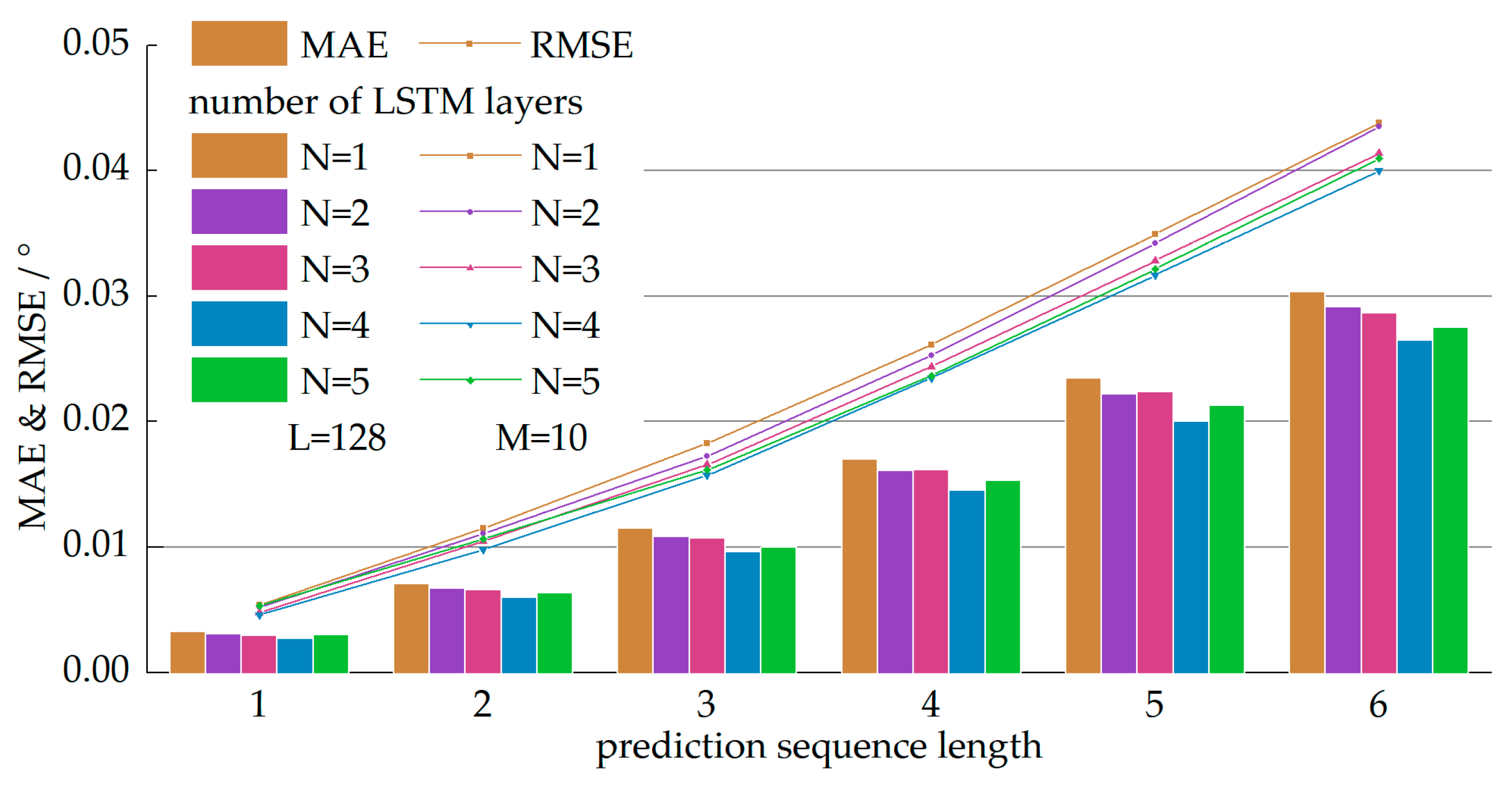
Figure 6, Figure 7 and Figure 8 illustrate the prediction performance of the models with different values of , , and , respectively. We evaluated the MAE and RMSE on each of the six timestamps. It was unsurprising to observe that the prediction error increased as the prediction length became longer. Figure 6 illustrates the performance of the models with a different number of hidden LSTM layers where the other two parameters were set as ,. As shown in Figure 6, the prediction performance became better with stacking of the LSTM layers. Generally, the prediction results yielded by deeper networks were more accurate, especially when the prediction length was long. Note that the LSTM network can be regarded as a deep neural network even when there is only one layer, due to the depth in time dimension. The best performance was yielded by the network with four hidden LSTM layers. Thus, we chose as the optimal value of the number of hidden LSTM layers.
Except for the depth of the network, the number of LSTM units in each layer also determines the complexity of the network and the number of variables, which significantly affects the prediction performance. Figure 7 shows the prediction error of models with a different number of LSTM units in each layer when and . Obviously, the lightweight network with 64 LSTM units in each layer was not competent enough to accomplish an accurate prediction. The overall prediction performance of the models with 256 and 512 units was close. Considering the complexity of the network, we chose as the optimal number of LSTM units in each layer.
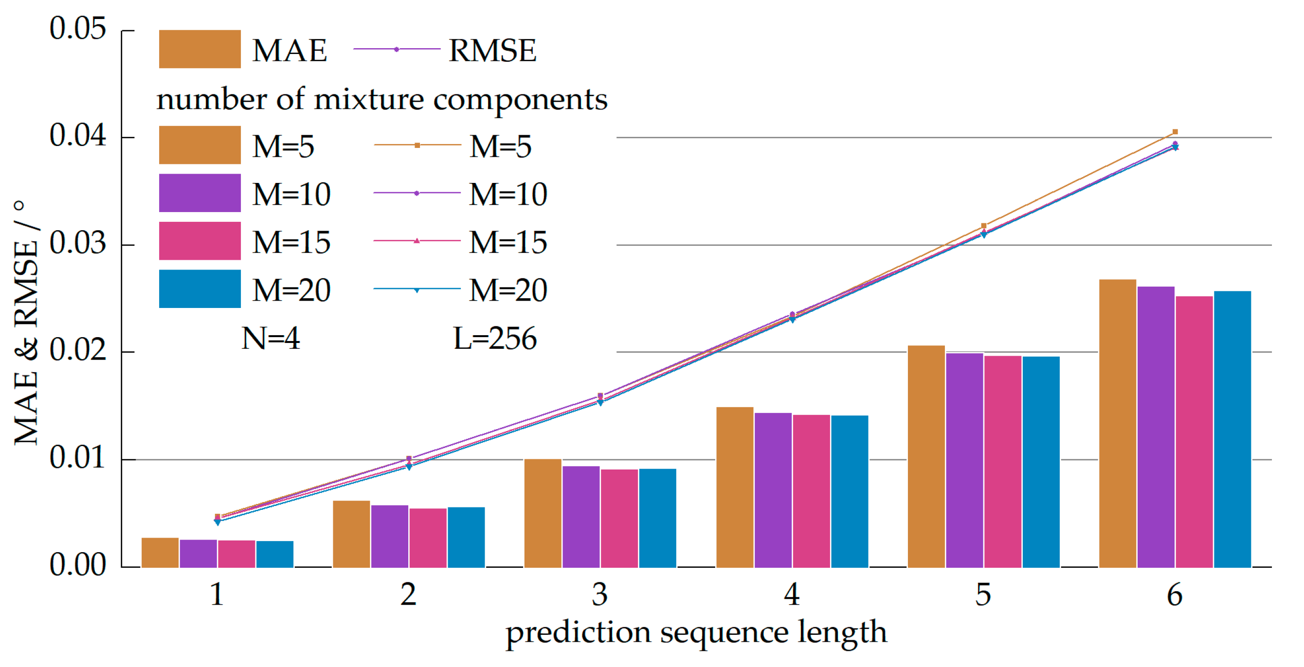
After determining the architecture parameters of the LSTM layers, we tested the models with a different number of mixture components in the MDN layer. The test performance is shown in Figure 8. Although the overall performance is promoted by adding mixture components, the promotion effect was not evident when compared to and . The prediction performance of the models with and were almost the same. The number of trainable variables in the MDN layer was proportional to . Thus, we determined as the optimal number of mixture components based on the tradeoff between prediction performance and the volume of the variable set.
The optimal parameter configuration of the BiRMDN is set out in Table 1.
4.3. Comparative Study with Other Approaches
In order to evaluate the performance of the BiRMDN model comparatively, we introduced three widely used prediction approaches for comparison including the bidirectional LSTM (BiLSTM) network, full-connected deep neural network (FCDNN) [37], and autoregressive moving average (ARMA) model [38].
The BiLSTM network is as described in Section 3.3. The difference between the BiLSTM and BiRMDN lies in the fact that the output of the BiLSTM is a concrete value of predicted offsets rather than the parameters of mixture probability distribution. In this experiment, the structure configuration and the related parameters of the BiLSTM were the same as the BiRMDN.
The full-connected neural network is frequently applied to prediction issues. Unlike the RNN, neurons in the same layer in a full-connected neural network are independent of each other. Connections only exist between neurons belonging to adjacent layers. Thus, the structural characteristics of the FCDNN determine its lack of ability to learn the contextual knowledge from the location sequence. We constructed the structure of the FCDNN with the same parameters as the BiRMDN.
In the trajectory preprocessing step, we converted the absolute coordinate sequence into an offset sequence. The ARMA (autoregressive moving average) model excels at modeling and predicting the offset sequence, which is a stationary sequence without tendency. The ARMA consists of two parts: autoregressive (AR) and moving average (MA). In the modeling phase, the ARMA captures both the autocorrelation features and noise features of the history sequence, then it utilizes these features to make predictions in the prediction phase.
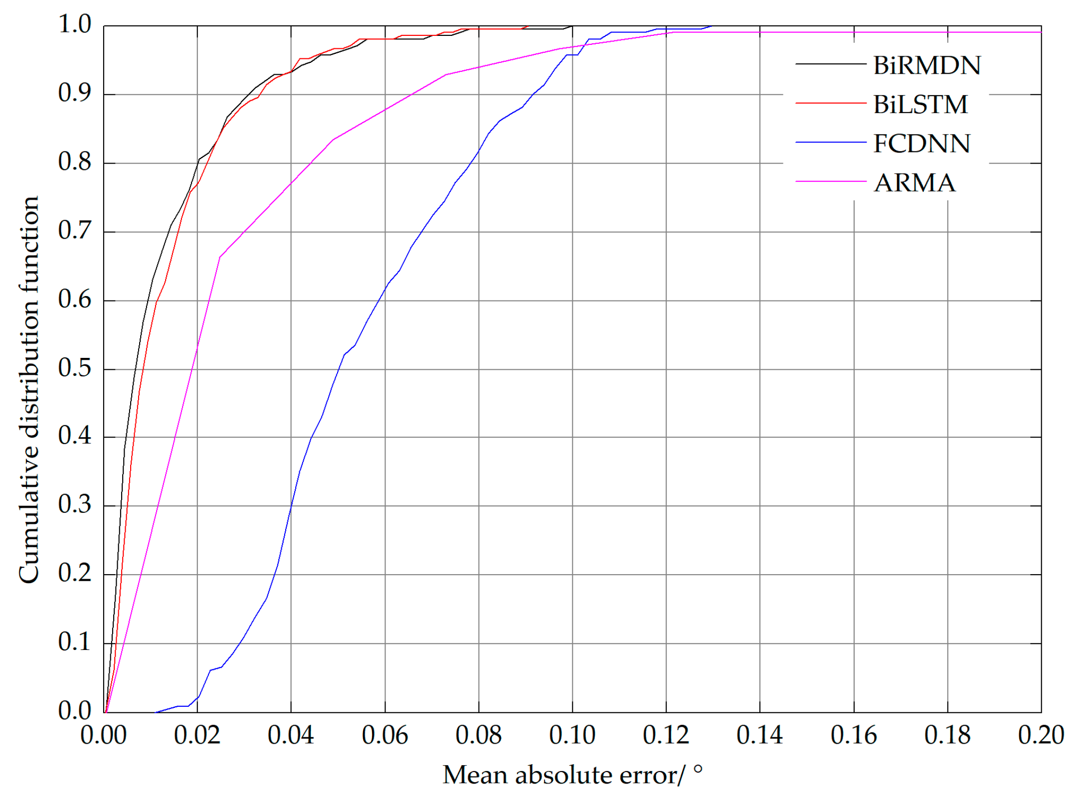
The performance comparison of these prediction experiments is reported in Table 2. As shown in Table 2, the BiRMDN model proposed in this work yielded the best overall performance. It is obvious that the evolution tendency of the prediction errors of these methods was similar over the six timestamps. With the increase in prediction length, the errors became larger. Compared to the FCDNN and ARMA groups, the experiments involving the LSTM network demonstrated that the long-term spatiotemporal dependency and contextual information captured by the LSTM are crucial for prediction. The prediction errors of the BiLSTM were lower than that of the BiRMDN when the prediction length was short, especially at the first timestamp. However, with the advance in prediction time, the prediction errors of the BLSTM diverged faster than that of the BiRMDN. The BiRMDN was proven to be superior in long-term prediction. In order to evaluate the overall performance of these methods more intuitively, we depicted the cumulative distribution function (CDF) of the mean absolute error over six predicted timestamps, as shown in Figure 9. The groups of the BiRMDN and BiLSTM resulted in a significant performance improvement when compared to the FCDNN and ARMA. It is also evident in Figure 9 that the overall performance of the BiRMDN was superior to that of the BiLSTM. In the experiments of the BiRMDN, the mean absolute error of more than 90% of the test trajectory segments was lower than 0.03° and more than 80% was lower than 0.02°.
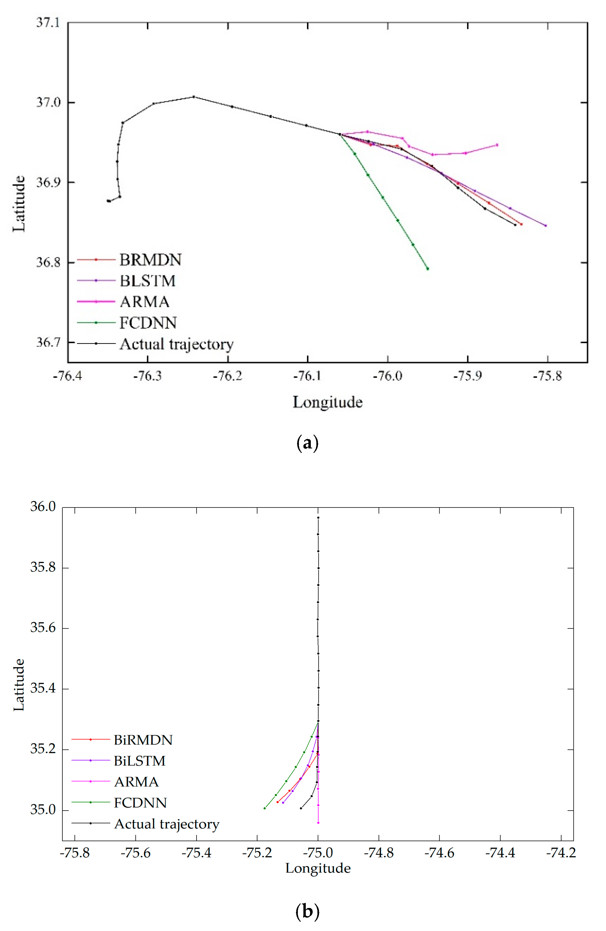
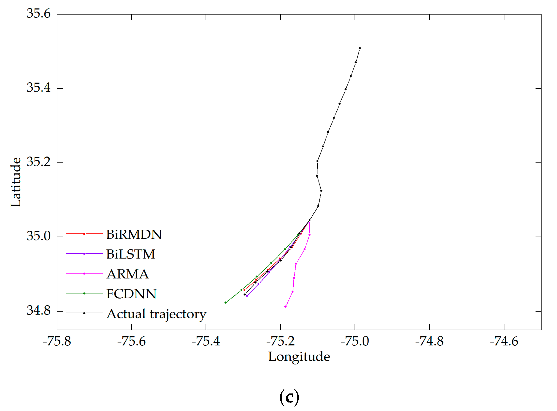
Figure 10 shows the prediction results of three test trajectory segments. The trajectory segment shown in Figure 10a curved in both the known input part and the part to be predicted. Obviously, both the FCDNN and ARMA failed to learn the evolution tendency of the trajectory due to the irregularity of the input signal. Although the prediction results of the BiLSTM were approximately in the same direction with the actual trajectory, it still failed to match the bending point. The discrepancy between the ground truth and the BiLSTM prediction was also obvious at each timestamp. As expected, the predicted locations of the BiRMDN were closest to the actual locations, especially at the bending point. Figure 10b shows the scenario where the known part is straight and uniform while the part to be predicted is inflected. This kind of inflection is tricky to predict. Only the BiRMDN, BiLSTM, and FCDNN successfully predicted the occurrence of inflection. Although the errors were relatively large for all of the methods, the BiRMDN still yielded the closest results. Figure 10c shows a uniform trajectory with a tiny radian, which the BiRMND, BiLSTM, and FCDNN all predicted well. Furthermore, the prediction errors of the BiRMDN were the lowest.
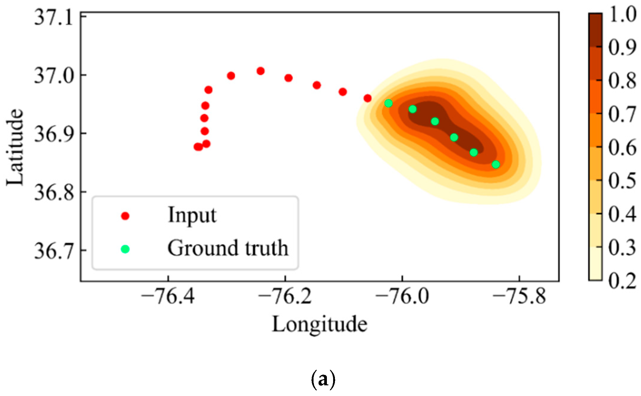
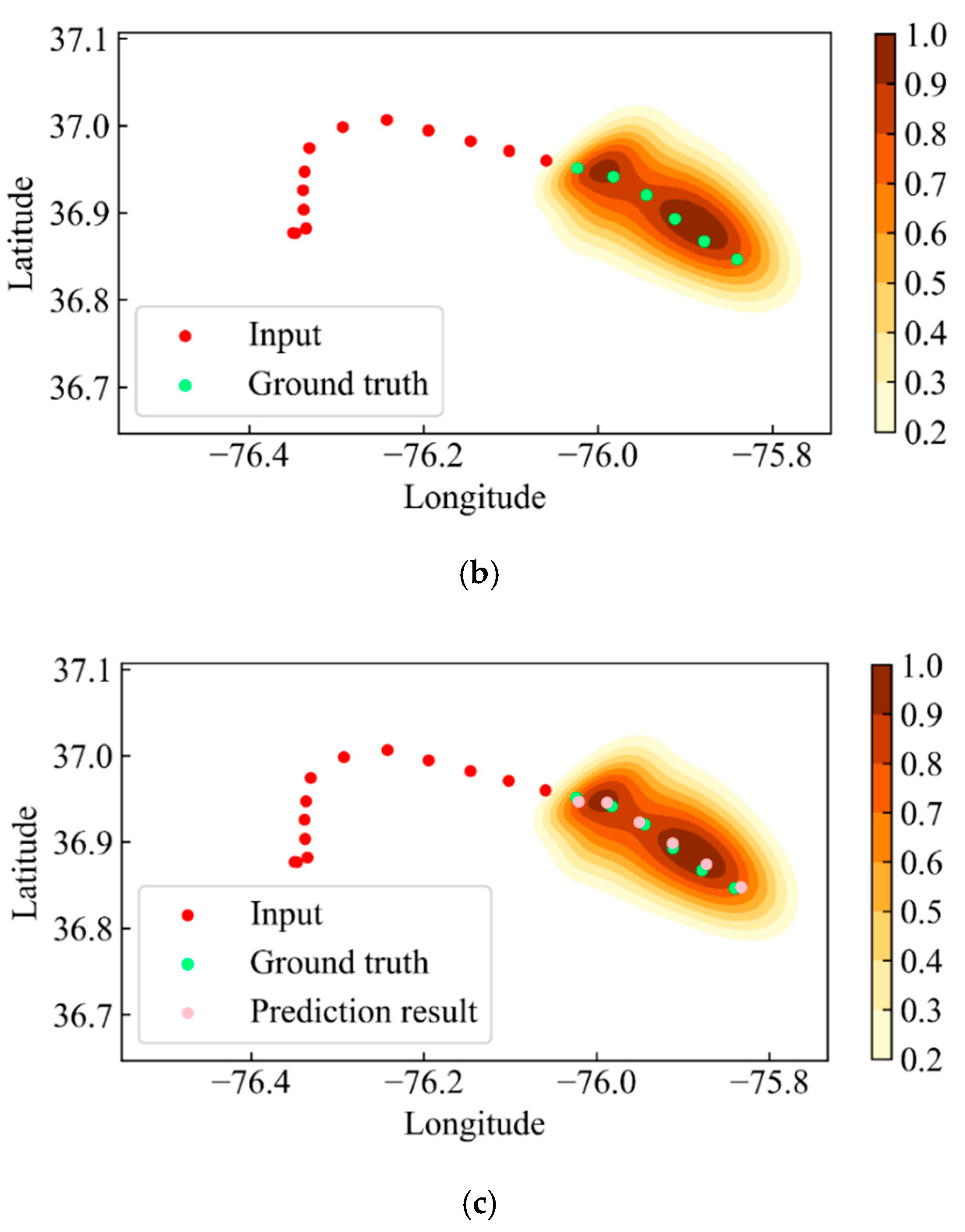
Visualizing the output of the Gaussian mixture distribution helps to comprehend the mechanism by which the BiRMDN performs location prediction. We depict the sampling process of obtaining the ultimate results from the mixture distribution in Figure 11. As shown in Figure 11, the red points and the green points denote the input locations and the ground truth, respectively; the contour is the normalized probability density distribution. When the incomplete trajectory segment is fed into the model, a set of parameters of Gaussian mixture distribution are generated. These parameters are further used to model the distribution of each predicted location, as shown in Figure 11a. Then, we employed the roulette strategy based on the weights to determine which Gaussian component would provide the final prediction results. The chosen Gaussian component is the contour shown in Figure 11b. Ultimately, we obtained the final predicted locations, the pink points shown in Figure 11c, by sampling from the chosen Gaussian distribution.
5. Discussion and Conclusions
We dedicated this paper to the location prediction method in a deep learning manner, the core of which was the construction of the BiRMDN model. This method predicted the future locations of moving objects based on trajectory mining. A trajectory mining method including trajectory preprocessing, construction of the BiRMDN model, and post-processing was presented. A vessel trajectory dataset was employed for the evaluation of this method. We performed parameter analysis to determine the optimal configuration of the BiRMDN in the experiments. In the comparative study with other widely used techniques, our method yielded promising results and the best performance, which demonstrates the superiority of the BiRMDN.
The BiRMDN model has three prominent highlights compared to previous methods. First, it has the ability to learn the long-term dependency and contextual information of trajectories, which significantly improves the prediction accuracy. Second, the output in the form of mixture probability distribution is efficient in modeling trajectories. The fuzzy prediction of locations is closer to the real mobility behavior. This model can also solve the challenging issue of predicting real-valued coordinates and avoid the curse of dimensionality. Finally, this model is expected to be easily implemented to different scenarios since the learning process is automatic without any hand-crafted feature engineering.
This work provides a typical method for practical location prediction applications, which can help in many practical fields such as traffic surveillance and early warning, abnormal trajectory detection, etc. For future work, the prediction model can be extended by adding more information such as the fusion information of the spatiotemporal and semantic context to accomplish prediction tasks in different hierarchical levels.
Author Contributions
Conceptualization, Rui Chen and Mingjian Chen; Data curation, Naikun Guo; Methodology, Rui Chen; Software, Rui Chen; Writing—original draft, Rui Chen; Writing—review & editing, Mingjian Chen and Wanli Li. All authors have read and agreed to the published version of the manuscript.
Acknowledgments
The authors would like to thank the U.S. Coast Guard Navigation Center for providing access to the AIS data.
Conflicts of Interest
The authors declare no conflicts of interest.
References
- Georgiou, H.; Karagiorgou, S.; Kontoulis, Y.; Pelekis, N.; Petrou, P.; Scarlatti, D.; Theodoridis, Y. Moving objects analytics: Survey on future location & trajectory prediction methods. arXiv 2018, arXiv:1807.04639. [Google Scholar]
- Bao, J.; Zheng, Y.; Mokbel, M.F. Location-based and preference aware recommendation using sparse geo-social networking data. In Proceedings of the 20th International Conference of Advances in Geographic Information Systems, Redondo Beach, CA, USA, 6–9 November 2012; pp. 199–208. [Google Scholar]
- Besse, P.C.; Guillouet, B.; Loubes, J.; Royer, F. Destination prediction by trajectory distribution based model. IEEE Trans. Intell. Transp. Syst. 2018, 19, 2470–2481. [Google Scholar] [CrossRef] [Green Version]
- Perera, L.P.; Oliveira, P.; Soares, C.G. Maritime traffic monitoring based on vessel detection, tracking, state estimation, and trajectory prediction. IEEE Trans. Intell. Transp. Syst. 2012, 13, 1188–1200. [Google Scholar] [CrossRef]
- Zhang, Z.; Yang, R.; Fang, Y. LSTM network based on antlion optimization and its application in flight trajectory prediction. In Proceedings of the 2nd IEEE Advanced IMCEC. Conference, Xi’an, China, 25–27 May 2018; pp. 1658–1662. [Google Scholar]
- Zheng, Y. Trajectory data mining: An overview. ACM Trans. Intell. Syst. Tech. 2015, 6, 1–41. [Google Scholar] [CrossRef]
- Wu, R.; Luo, G.; Shao, J.; Tian, L.; Peng, C. Location prediction on trajectory data: A review. Big Data Min. Anal. 2018, 1, 108–127. [Google Scholar]
- Li, Y.; Zheng, Y.; Zhang, H.; Chen, L. Traffic prediction in a bike-sharing system. In Proceedings of the 23rd International Conference Advances in Geographic Information Systems, Seattle, WA, USA, 3–6 November 2015; pp. 1–10. [Google Scholar]
- Monreale, A.; Pinelli, F.; Trasarti, R.; Giannotti, F. WhereNext: A location predictor on trajectory pattern mining. In Proceedings of the 15th ACM SIGKDD International Conference on KDD, Paris, France, 28 June–1 July 2009; pp. 637–646. [Google Scholar]
- Morzy, M. Mining frequent trajectories of moving objects for location prediction. In Proceedings of the 5th International Conference on Machine Learning and Data Mining in Pattern Recognition, Leipzig, Germany, 18–20 July 2007; pp. 667–680. [Google Scholar]
- Wu, F.; Fu, K.; Wang, Y.; Xiao, Z.; Fu, X. A spatial-temporal-semantic neural network algorithm for location prediction on moving objects. Algorithms 2017, 10, 37. [Google Scholar] [CrossRef] [Green Version]
- Kormahalleh, M.M.; Sefidmazgi, M.G.; Homaifar, A. A sparse recurrent neural network for trajectory prediction of Atlantic hurricanes. In Proceedings of the Genetic and Evolutionary Computation Conference, Denver, CO, USA, 20–24 July 2016; pp. 957–964. [Google Scholar]
- Song, L.; Kotz, D.; Jain, R.; He, X. Evaluating location predictors with extensive Wi-Fi mobility data. In Proceedings of the 23rd Annual Joint Conference of the IEEE Computer and Communications Societies, Hong Kong, China, 7–11 March 2004; pp. 1414–1424. [Google Scholar]
- Sutskever, I.; Martens, J.; Hinton, G.E. Generating text with recurrent neural networks. In Proceedings of the 28th International Conference of Machine Learning, Bellevue, WA, USA, 28 June–2 July 2011; pp. 1017–1024. [Google Scholar]
- Krizhevsky, A.; Sutskever, I.; Hinton, G.E. ImageNet classification with deep convolutional neural networks. In Proceedings of the Advances in Neural Information Processing Systems, Lake Tahoe, CA, USA, 3–6 December 2012; pp. 1097–1105. [Google Scholar]
- Cuttone, A.; Lehmann, S.; González, M.C. Understanding predictability and exploration in human mobility. EPJ Data Sci. 2018, 7, 1–17. [Google Scholar] [CrossRef] [Green Version]
- Hochreiter, S.; Schmidhuber, J. Long short-term memory. Neural Comput. 1997, 9, 1735–1780. [Google Scholar] [CrossRef]
- Bishop, C.M. Mixture Density Networks; Aston University: Birmingham, UK, 1994. [Google Scholar]
- Chen, R.; Chen, M.; Li, W.; Wang, J.; Yao, X. Mobility modes awareness from trajectories based on clustering and a convolutional neural network. ISPRS Int. J. Geo-Inf. 2019, 8, 208. [Google Scholar] [CrossRef] [Green Version]
- Ashbrook, D.; Starner, T. Using GPS to learn significant locations and predict movement across multiple users. Pers. Ubiquitous Comput. 2003, 7, 275–286. [Google Scholar] [CrossRef]
- Mathew, W.; Raposo, R.; Martins, B. Predicting future locations with hidden Markov models. In Proceedings of the ACM Conference of Ubiquitous Computation, Pittsburgh, PA, USA, 5–8 September 2012; pp. 911–918. [Google Scholar]
- Qiao, S.; Shen, D.; Wang, X.; Han, N.; Zhu, W. A self-adaptive parameter selection trajectory prediction approach via hidden Markov models. IEEE Trans. Intell. Transp. Syst. 2015, 16, 284–296. [Google Scholar] [CrossRef]
- Ying, J.J.; Lee, W.; Tseng, V.S. Mining geographic-temporal-semantic patterns in trajectories for location prediction. ACM Trans. Intell. Syst. Technol. 2013, 5, 1–33. [Google Scholar] [CrossRef]
- Lei, P.; Li, S.; Peng, W. QS-STT: QuadSection clustering and spatial-temporal trajectory model for location prediction. Distrib. Parallel Databases 2013, 31, 231–258. [Google Scholar] [CrossRef]
- Nguyen, D.; Van, C.L.; Ali, M.I. Vessel trajectory prediction using sequence-to-sequence models over spatial grid. In Proceedings of the 12th ACM International Conference on DEBS, Hamilton, New Zealand, 25–29 June 2018; pp. 258–261. [Google Scholar]
- Wu, H.; Chen, Z.; Sun, W.; Zheng, B.; Wang, W. Modeling trajectories with recurrent neural networks. In Proceedings of the 26th IJCAI, Melbourne, Australia, 19–25 August 2017; pp. 3083–3090. [Google Scholar]
- Liu, Q.; Wu, S.; Wang, L.; Tan, T. Predicting the next location: A recurrent model with spatial and temporal contexts. In Proceedings of the 30th AAAI Conference, Phoenix, AZ, USA, 12–17 February 2016; pp. 194–200. [Google Scholar]
- Feng, J.; Li, Y.; Zhang, C.; Sun, F.; Meng, F.; Guo, A.; Jin, D. DeepMove: Predicting human mobility with attentional recurrent networks. In Proceedings of the World Wide Web Conference, Lyon, France, 23–27 April 2018. [Google Scholar]
- Graves, A. Generating sequences with recurrent neural networks. arXiv 2013, arXiv:1308.0850. [Google Scholar]
- Zhao, Y.; Yang, R.; Chevalier, G.; Shah, R.; Romijnders, R. Applying deep bidirectional LSTM and mixture density network for basketball trajectory prediction. OPTIK 2018, 158, 266–272. [Google Scholar] [CrossRef] [Green Version]
- Xu, J.; Rahmatizadeh, R.; Bölöni, L.; Turgut, D. Real-time prediction of taxi demand using recurrent neural networks. IEEE Trans. Intell. Transp. Syst. 2018, 19, 2572–2581. [Google Scholar] [CrossRef]
- Graves, A.; Schmidhuber, J. Framewise phoneme classification with bidirectional LSTM and other neural network architectures. Neural Netw. 2005, 18, 602–610. [Google Scholar] [CrossRef]
- Pascanu, R.; Mikolov, T.; Bengio, Y. On the difficulty of training recurrent neural networks. arXiv 2013, arXiv:1211.5063. [Google Scholar]
- Hinton, G.E.; Srivastava, N.; Krizhevsky, A.; Sutskever, I.; Salakhutdinov, R.R. Improving neural networks by preventing co-adaptation of feature detectors. arXiv 2012, arXiv:1207.0580. [Google Scholar]
- MarineCadastre.gov. Available online: https://marinecadastre.gov/ais/ (accessed on 5 January 2020).
- Kingma, D.P.; Ba, J.L. Adam: A method for stochastic optimization. In Proceedings of the International Conference on Learning Representations, San Diego, CA, USA, 7–9 May 2015; pp. 1–15. [Google Scholar]
- Endo, Y.; Toda, H.; Nishida, K.; Ikedo, J. Classifying spatial trajectories using representation learning. Int. J. Data Sci. Anal. 2016, 2, 107–117. [Google Scholar] [CrossRef] [Green Version]
- Navarro-Moreno, J. ARMA prediction of widely linear systems by using the innovations algorithm. IEEE Trans. Signal Process. 2008, 56, 3061–3068. [Google Scholar] [CrossRef]
Figure 1.
Process of the proposed method. BiRMDN: bidirectional recurrent mixture density network.

Figure 2.
Schematic of generating the training data and test data when input sequence length , prediction length . (a) Generating training input and label with a sliding window. (b) Test input, ground truth, and prediction results.
Figure 2.
Schematic of generating the training data and test data when input sequence length , prediction length . (a) Generating training input and label with a sliding window. (b) Test input, ground truth, and prediction results.

Figure 3.
Schematic of unfolded structure of bidirectional recurrent mixture density network (BiRMDN). LSTM: long-short term memory, MDN: mixture density network.
Figure 3.
Schematic of unfolded structure of bidirectional recurrent mixture density network (BiRMDN). LSTM: long-short term memory, MDN: mixture density network.

Figure 4.
The architecture of the long short-term memory (LSTM) unit.

Figure 5.
The study region (from N31.8° to N37.3° and W74.3° to W78°) and trajectory data generated by vessels traveling back and forth between the Florida Strait and Port of Virginia from 1 May to 31 August 2014.
Figure 5.
The study region (from N31.8° to N37.3° and W74.3° to W78°) and trajectory data generated by vessels traveling back and forth between the Florida Strait and Port of Virginia from 1 May to 31 August 2014.

Figure 6.
Performance of the models with a different number of hidden LSTM layers where , . The horizontal axis denotes the prediction sequence length. The vertical axis denotes the value of the MAE and RMSE. The bars represent the value of the MAE and the solid lines represent the value of the RMSE.

Figure 7.
Performance of the models with a different number of LSTM units in each layer where , . The horizontal axis denotes the prediction sequence length. The vertical axis denotes the value of the MAE and RMSE. The bars represent the value of the MAE and the solid lines represent the value of the RMSE.

Figure 8.
Performance of models with a different number of mixture components where , . The horizontal axis denotes the prediction sequence length. The vertical axis denotes the value of the MAE and RMSE. The bars represent the value of the MAE and the solid lines represent the value of the RMSE.
Figure 8.
Performance of models with a different number of mixture components where , . The horizontal axis denotes the prediction sequence length. The vertical axis denotes the value of the MAE and RMSE. The bars represent the value of the MAE and the solid lines represent the value of the RMSE.

Figure 9.
Cumulative distribution function (CDF) of the mean absolute error over six predicted locations.
Figure 9.
Cumulative distribution function (CDF) of the mean absolute error over six predicted locations.

Figure 10.
Instances of the prediction results of three different trajectories. (a) Curving trajectory. (b) Trajectory with inflection. (c) Uniform trajectory.
Figure 10.
Instances of the prediction results of three different trajectories. (a) Curving trajectory. (b) Trajectory with inflection. (c) Uniform trajectory.


Figure 11.
Visualization of the sampling process from the output of the BiRMDN. (a) Generating mixture distribution. (b) Determining the Gaussian component. (c) Sampling from the chosen Gaussian distribution.
Figure 11.
Visualization of the sampling process from the output of the BiRMDN. (a) Generating mixture distribution. (b) Determining the Gaussian component. (c) Sampling from the chosen Gaussian distribution.


Table 1.
The optimal parameter configuration of the BiRMDN model. BiRMDN: bidirectional recurrent mixture density network.
Table 1.
The optimal parameter configuration of the BiRMDN model. BiRMDN: bidirectional recurrent mixture density network.
| Parameters | Value |
|---|---|
| Number of hidden LSTM layers | 4 |
| Number of LSTM units in each layer | 256 |
| Number of mixture components | 15 |
| Dropout probability | 0.2 |
| Optimizer | Adam |
| Loss function | Negative log likelihood |
| Initial learning rate | 0.001 |
| Decay rate (per epoch) | 0.98 |
Table 2.
Prediction performance of the comparative experiments.
| Steps | MAE (°) | RMSE (°) | ||||||
|---|---|---|---|---|---|---|---|---|
| BiRMDN | BiLSTM | ARMA | FCDNN | BiRMDN | BiLSTM | ARMA | FCDNN | |
| 1 | 0.00255 | 0.00253 | 0.01680 | 0.01572 | 0.00456 | 0.00420 | 0.09220 | 0.01699 |
| 2 | 0.00553 | 0.00602 | 0.02098 | 0.03189 | 0.00953 | 0.00954 | 0.09321 | 0.03467 |
| 3 | 0.00915 | 0.01018 | 0.02661 | 0.04761 | 0.01554 | 0.01538 | 0.09534 | 0.05171 |
| 4 | 0.01422 | 0.01551 | 0.03286 | 0.06336 | 0.02321 | 0.02288 | 0.09851 | 0.06882 |
| 5 | 0.01970 | 0.02141 | 0.04035 | 0.07976 | 0.03117 | 0.03094 | 0.10339 | 0.08681 |
| 6 | 0.02526 | 0.02753 | 0.04894 | 0.09642 | 0.03910 | 0.03931 | 0.10971 | 0.10525 |
© 2020 by the authors. Licensee MDPI, Basel, Switzerland. This article is an open access article distributed under the terms and conditions of the Creative Commons Attribution (CC BY) license (http://creativecommons.org/licenses/by/4.0/).
Share and Cite
MDPI and ACS Style
Chen, R.; Chen, M.; Li, W.; Guo, N. Predicting Future Locations of Moving Objects by Recurrent Mixture Density Network. ISPRS Int. J. Geo-Inf. 2020, 9, 116. https://0-doi-org.brum.beds.ac.uk/10.3390/ijgi9020116
AMA Style
Chen R, Chen M, Li W, Guo N. Predicting Future Locations of Moving Objects by Recurrent Mixture Density Network. ISPRS International Journal of Geo-Information. 2020; 9(2):116. https://0-doi-org.brum.beds.ac.uk/10.3390/ijgi9020116
Chicago/Turabian StyleChen, Rui, Mingjian Chen, Wanli Li, and Naikun Guo. 2020. "Predicting Future Locations of Moving Objects by Recurrent Mixture Density Network" ISPRS International Journal of Geo-Information 9, no. 2: 116. https://0-doi-org.brum.beds.ac.uk/10.3390/ijgi9020116
Note that from the first issue of 2016, this journal uses article numbers instead of page numbers. See further details here.