The Indoor Localization of a Mobile Platform Based on Monocular Vision and Coding Images

Abstract

With the extensive development and utilization of urban underground space, coal mines, and other indoor areas, the indoor positioning technology of these areas has become a hot research topic. This paper proposes a robust localization method for indoor mobile platforms. Firstly, a series of coding graphics were designed for localizing the platform, and the spatial coordinates of these coding graphics were calculated by using a new method proposed in this paper. Secondly, two spatial resection models were constructed based on unit weight and Tukey weight to localize the platform in indoor environments. Lastly, the experimental results show that both models can calculate the position of the platform with good accuracy. The space resection model based on Tukey weight correctly identified the residuals of the observations for calculating the weights to obtain robust positioning results and has a high positioning accuracy. The navigation and positioning method proposed in this study has a high localization accuracy and can be potentially used in localizing practical indoor space mobile platforms.

1. Introduction

Localization is one of the core technologies for indoor surveying and mapping services [1,2]. In order to achieve accurate indoor navigation and positioning, many navigation and positioning technologies have been rapidly developed based on ultra wide band (UWB) [3,4], radio frequency (RF) [5,6], Wi-Fi [7,8], Bluetooth [9,10], vision [11,12], ZigBee [13,14], and multi-sensor combinations [15,16]. Vision sensors are a streaming media technology that can achieve rich texture information and transmit information in real time, which can be used to localize and collect environmental information, and have been used in the Chang’e III inspections of China and the spirit and opportunity rovers in America [17,18]). To date, the research on spatial navigation and positioning methods based on vision sensors has been experiencing intense development [19,20] and can be roughly classified into two groups. In one category, researchers take advantage of the landmarks present in the environment to estimate the camera matrix and extract the query location [21,22]. The other category includes the works that use a stored image database annotated with the position information of the cameras, such as image fingerprinting-based methods [23,24]. Common visual positioning methods include monocular positioning [25,26], binocular positioning [27], and RGB-D positioning [12,28]. Among them, the monocular vision positioning method only needs one camera to locate a position and uses either one single frame image or stereo images. Many researchers have studied monocular vision positioning technologies. For example, Liu et al. [29] proposed a self-localization method for indoor mobile robots based on artificial landmarks and binocular stereo vision. Royer et al. [25] studied the localization and automatic navigation methods for a mobile robot based on monocular vision and proposed that by using a monocular camera and natural landmark, the autonomous navigation of a mobile robot via manual guidance and learning can be achieved. Zhong et al. [30] presented a self-localization scheme used for indoor mobile robot navigation based on a reliable design and the recognition of artificial visual landmarks. Xiao et al. [31] proposed a method that can detect static objects in large indoor spaces and then calculate a smartphone’s position to locate its user. With the assistance of UWB, Ramirez et al. [32] proposed a relative localization method using computer vision and the UWB range for a flying robot and showed that the errors in the estimated relative positions were between ± 0.190 m on the x-East axis and ± 0.291 m on the z-North axis at a 95% confidence level. Tiemann et al. [33] proposed an enhanced UAV indoor navigation method using SLAM-augmented UWB localization, in which the SLAM-augmented UWB localization had a 90% quantile error of 13.9 cm.

In addition, positioning technologies based on visual sensors, such as structures from motion (SFM), simultaneous localization and mapping (SLAM), and visual odometers (VOs) have been widely studied. Rafael et al. [34] proposed a novel method to simultaneously solve the problems of mapping and localization using a set of squared planar markers. Experiments show that the proposed method performs better than the Structure from Motion and visual SLAM techniques. Lim et al. [35] proposed real-time single camera simultaneous localization and mapping (SLAM) using artificial landmarks. The technique of using natural features to perform indoor SLAM, however, is not yet mature enough for practical use, as it has too many exceptions and assumptions. Moreover, existing methods that use natural landmarks or features are very fragile due to data association failures. However, thanks to the proposed landmark model, which includes an identification code on the surface, data association is highly successful. Moreover, the 3D position of each landmark can be obtained from one frame of the image. In GPS-denied environments, it has been demonstrated that VO provides a relative position error ranging from 0.1% to 2% [19,36]. SLAM and VO technology are both types of relative positioning methods; it is usually necessary to cooperate with other sensors or control points to achieve absolute positioning.

The above review shows that many of the research methods that are based on monocular vision do not consider the influence of the residual size of the observations. As a result, the errors in the observation values obtained by visual methods cannot be detected, located, or rejected effectively, as this would lead to inaccurate results.

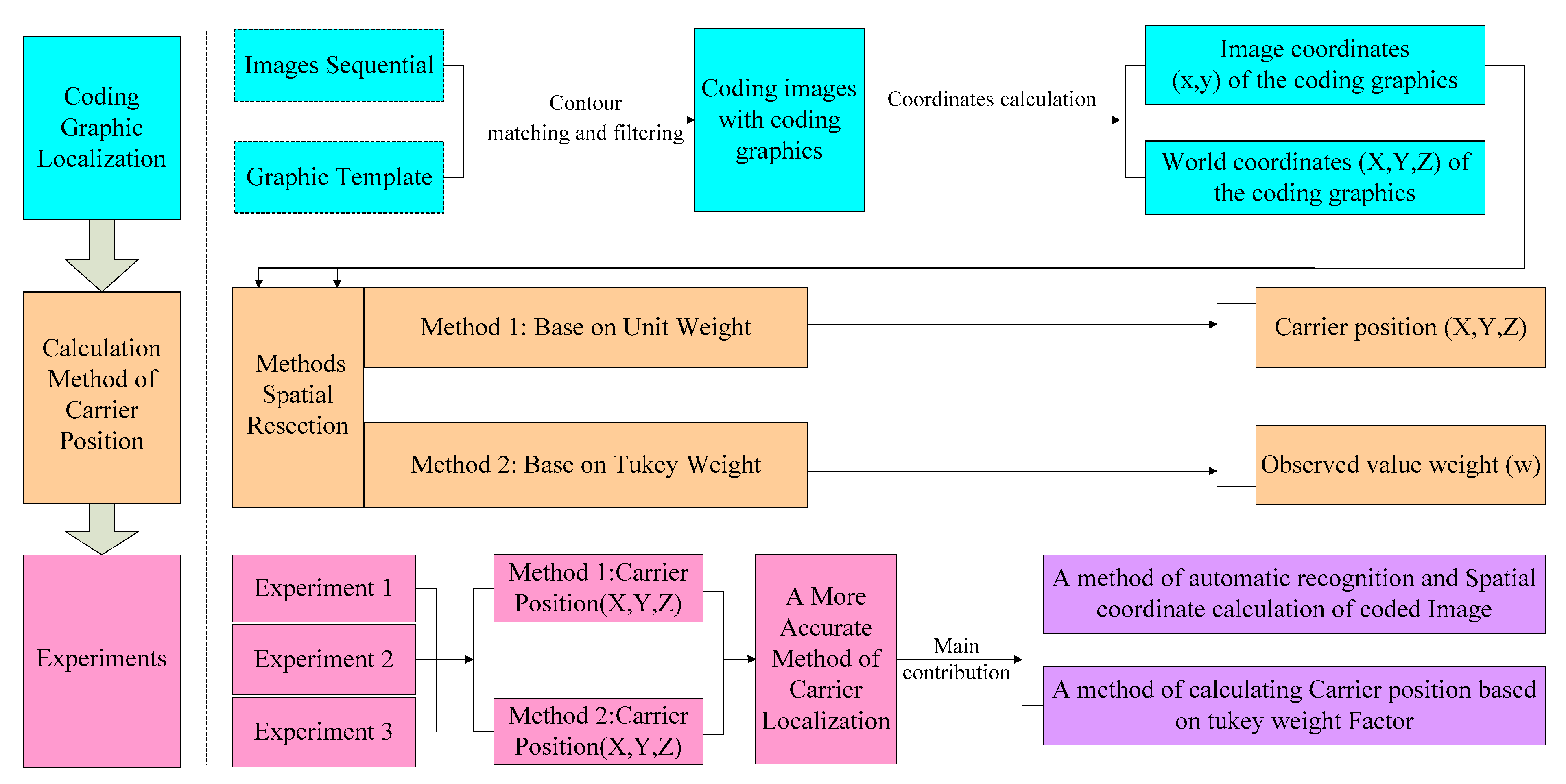
In order to overcome the above problems, this paper proposes a robust platform position measurement method based on coding graphics and a monocular vision sensor. This method can provide robust navigation and positioning services for an indoor mobile platform. The technical route for this method is shown in Figure 1. First, a series of coding graphics for the positioning of the platform is designed, and a method for calculating the spatial coordinates of the coding graphics is proposed. Secondly, two space resection models are constructed based on unit weight [37] and Tukey weight [37,38,39,40], respectively. Indoor test environments suitable for the static and dynamic positioning of the platform are then built, and static and dynamic positioning tests of the mobile platform are carried out. Finally, the position results of both methods are compared to the true values, and the feasibility and robustness of this paper’s methods are analysed by experiments. The main contributions of this study include a method for the automatic recognition and spatial coordinate calculations of coded images, as well as a method for calculating carrier position based on the Tukey weight factor.

The remainder of this paper is organized as follows. Section 2 briefly reviews the coding graphic localization and position calculation methods. The positioning experiments and discussion are carried out in Section 3. In Section 4, some conclusions related to the work are summarized.

2. Materials and Methods

An automatic location method based on vision and coding images is proposed in this paper. Coding graphics assume the role of control points in photogrammetry. In order to realize automatic positioning, it is necessary to be able to obtain the image and world coordinates of the coding graphics automatically. Then, a collinear equation is constructed based on the principle of image points, photography center, and object points in a straight line. Finally, positioning is realized based on the space rear resection method. The main content consists of two parts: coding graphic localization and position calculation methods. The details are as follows.

2.1. Coding Graphic Localization

2.1.1. Coding Graphic Design

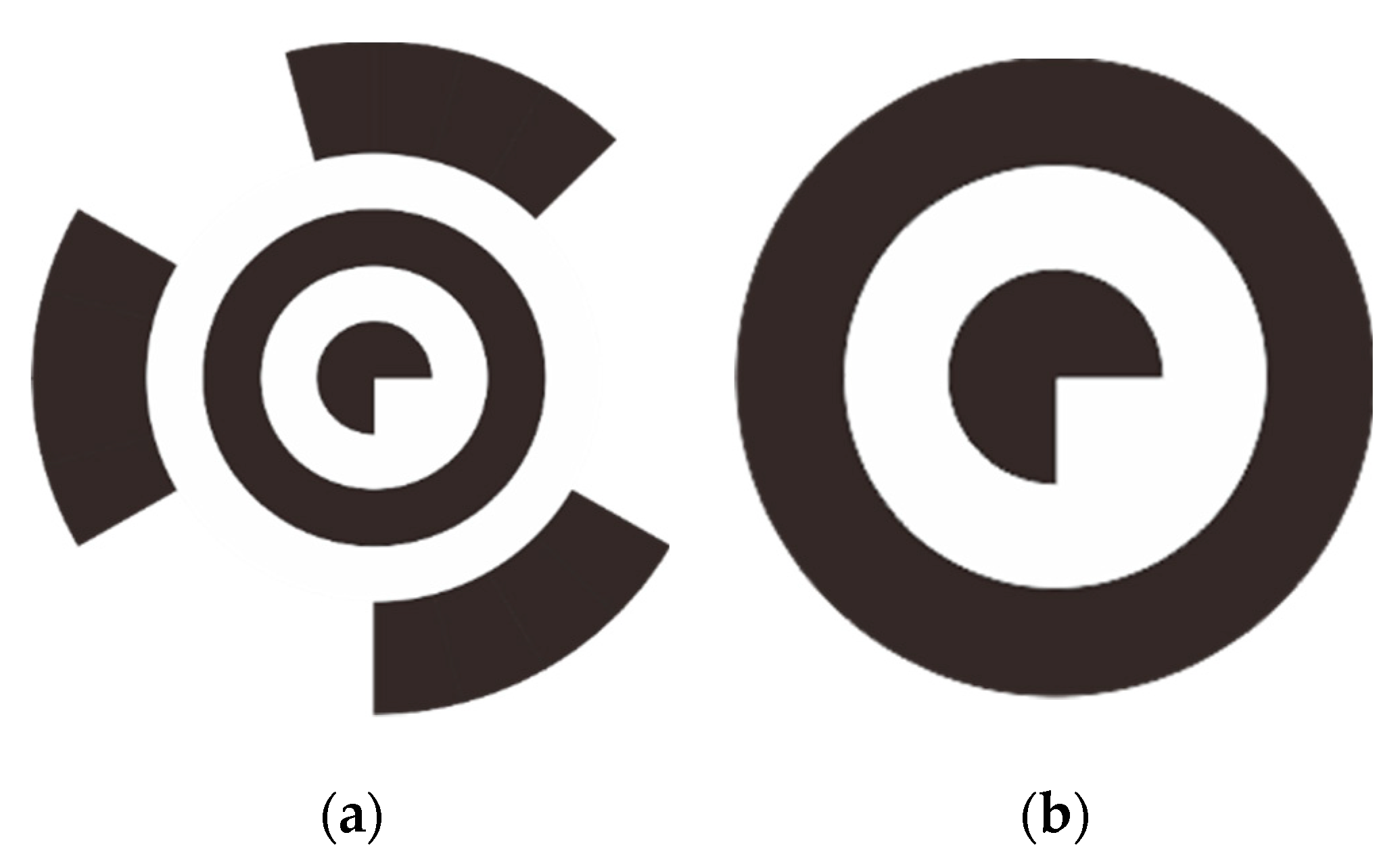
In order to provide indoor positioning information for indoor mobile platforms, this paper designs a series of coding graphics with black and white colors, shown in Figure 2a. The coding graphics include five layers. From the inside to the outside, the first layer is a black 3/4 circle, the second and fourth layers are white circular rings, the third layer is a black circular ring, and the fifth layer is a coding layer that is divided into 24 black and white equal parts. When the coding layer is used to represent a coding number, black means a binary 0 and white means a binary 1. The five layers have the same circular center. Every layer’s radius is R, except for the fifth layer, whose radius is 2R. According to the counterclockwise order, the coding number is made up of 24 ‘0’, and ‘1’. The coding quantities can be 2²⁴. The three inner layers comprise a template graphic, as shown in Figure 2b [41], which can be used to determine whether there is a coding graphic in the image.

Coding graphics can play the role of the controlling image, which is required to be able to automatically detect and identify the coding image, determine the coding numbers, and calculate the image and world coordinates for the central position of the graphics. Based on the method of space resection, three or more controlling images are needed to calculate the position of the camera. In addition, the even distribution of the control points on the image would be more helpful to improve the accuracy of the positioning results. The world coordinates of each graphic are measured by an electronic total station, which is a surveying and mapping instrument system.

2.1.2. Coding Graphic Identification and Localization

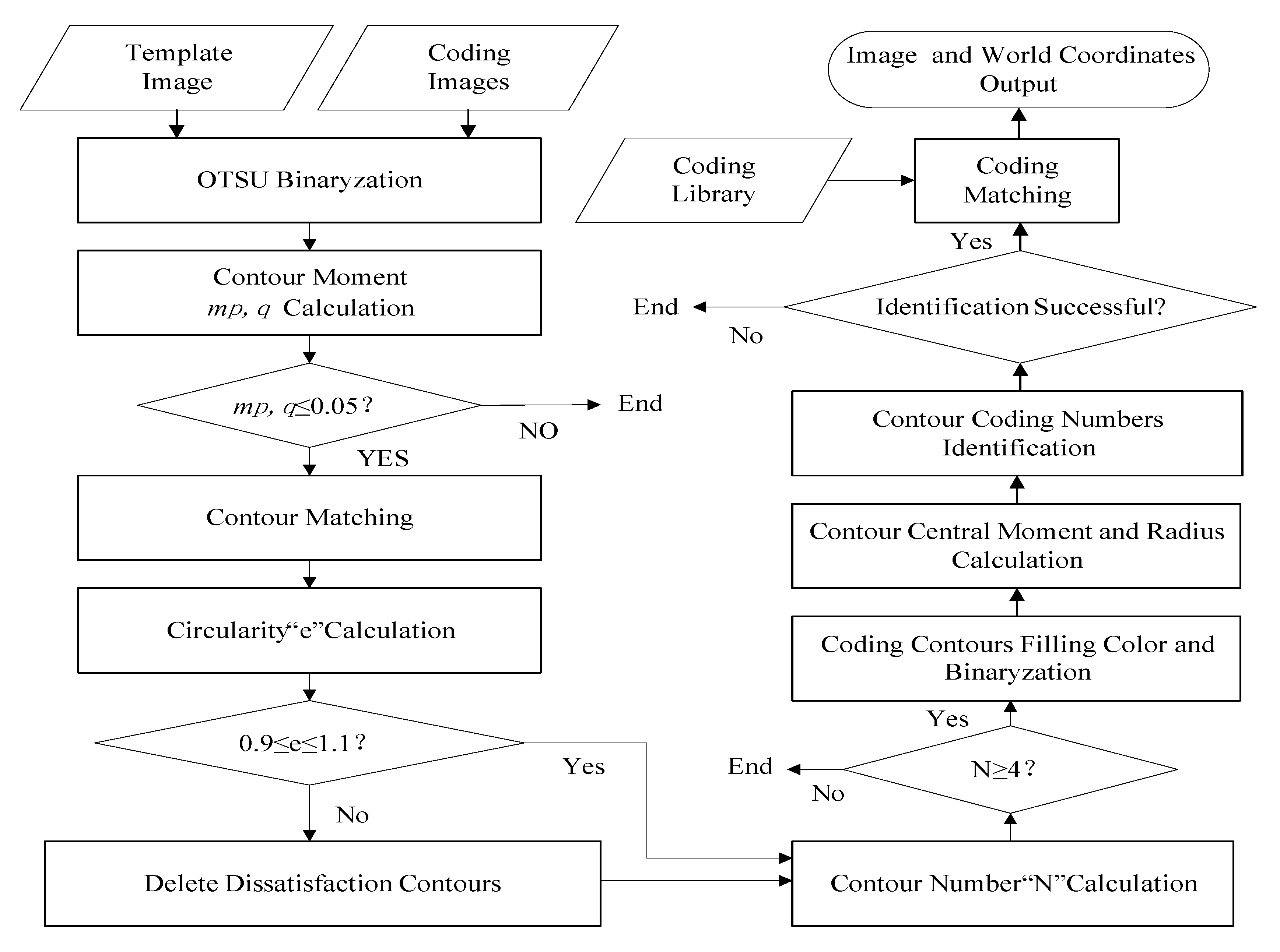
This paper proposes an automatic identification and extraction method for coding graphics and their spatial coordinates, including coding graphic recognition based on contour matching [42], the moment value [43], and the roundness threshold judgment [43], as well as an automatic extraction of the image coordinates of the coding graphics based on the contour centre moment, and a method to map the world coordinates of the coding graphics to the coding graphics database. The flowchart is shown in Figure 3.

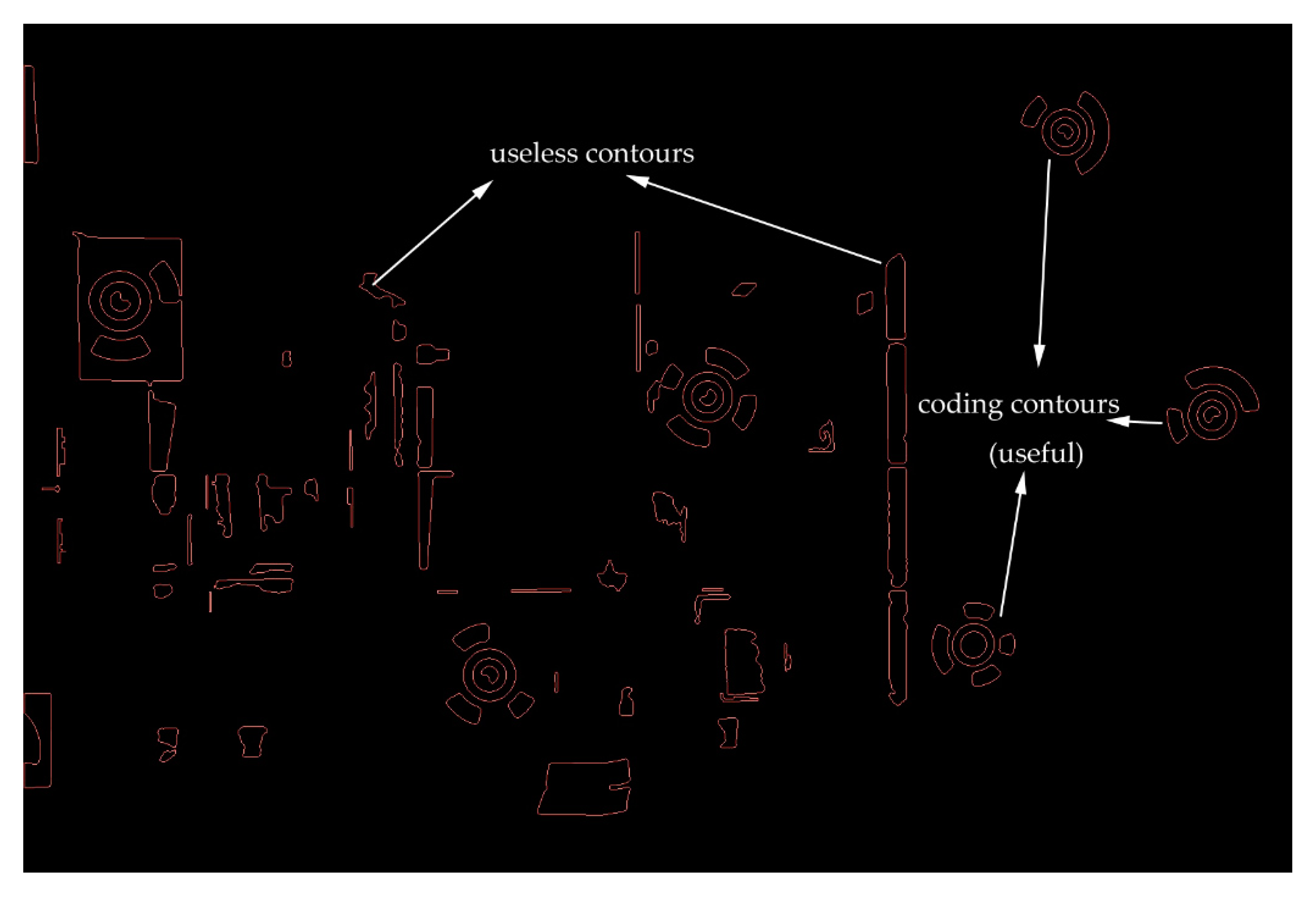
In this paper, the contour-matching method is used to traverse the coding graphics from the coding image shown in Figure 4, and the similarity between the template graphic and the coding graphics on the coding image is judged according to the calculated moment. If the calculated moment satisfies the threshold setting, then the contour matching is performed; otherwise, the calculation is terminated. In the process of contour matching, whether the contour is available or not is judged according to its roundness. If its roundness does not meet the threshold setting, the contour is defined as a useless profile and deleted. If the threshold setting is met, the number of contours that meet the requirements is calculated, requiring the number of contours to be no less than four; if not, the calculation is terminated. The contour radius is calculated according to the relationship between the contour perimeter and the area, and the coordinate observation value of the centre point of the coded graph is calculated according to the contour centre moment. According to the method in this paper, the contour coding sequence can be identified and determined. By using the method to map the world coordinates of the coding graphics to the coding graphics database, the world coordinates of the centre points of the encoded graphics are obtained.

The main processes of contour matching, contour filtering, and spatial coordinate acquisition are as follows.

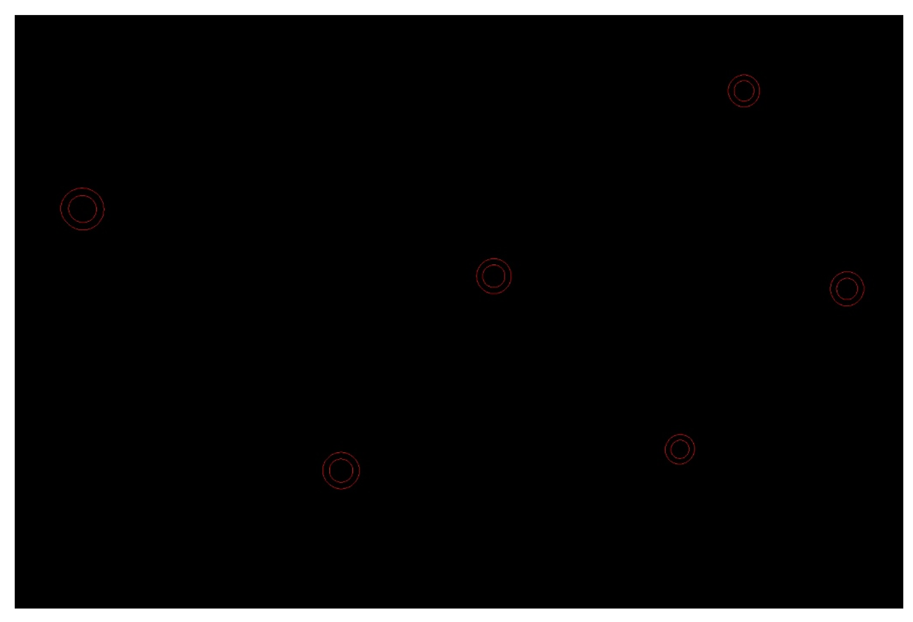
Contour matching [42]: The coding graphics can be searched and located using contour matching. In the matching process, if the contour moment [43] represented by ${\mathrm{m}}_{p,q}$ is inversely proportional to the similarity, then the smaller the value, the higher the similarity: the experiment shows that 0.05 has a better effect and satisfies the requirements of the threshold value. In this case, the matching process will continue; otherwise, it will be stopped [44]. Figure 5 shows the results of the matching.

$${\mathrm{m}}_{p,q}={\displaystyle \sum }_{i=1}^{n}I\left(x,y\right)x^p{y}^q$$

(1)

where moment $p$ corresponds to the $x$ dimension, and moment $q$ corresponds to the $y$ dimension. The orders represent the indices of the corresponding parts.

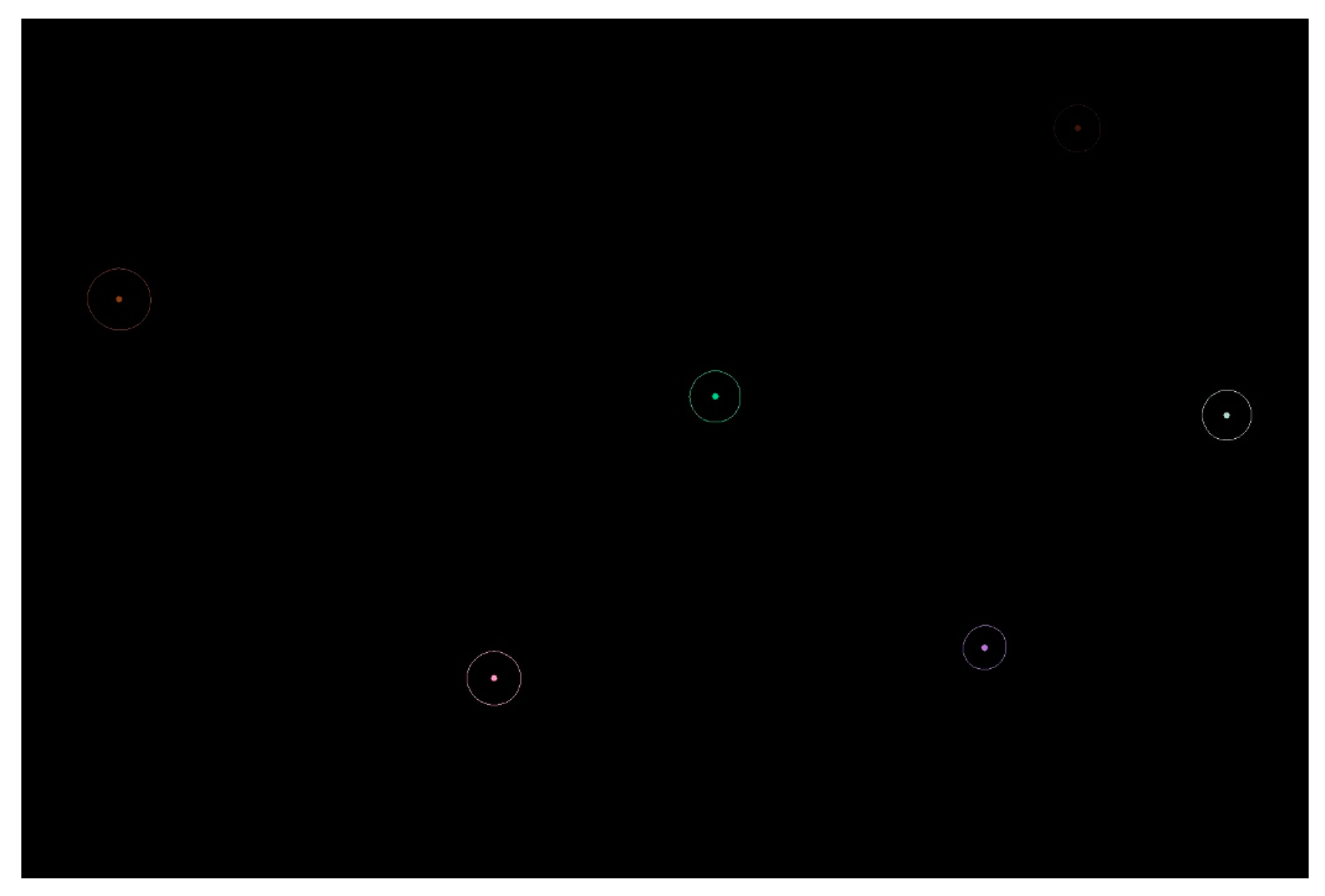
Contour filtering: If circularity ‘e’ [43] does not meet the threshold value, the contour will be defined as a useless profile that is not a circle or an ellipse, as shown in Figure 5, and will be deleted. If the quantities of the contours are less than 4, the calculation will be terminated.

$$e=\frac{4\pi S}{C^2}$$

(2)

where S is the area of a contour, and C is the length of the contour. Thus, the circularity of a circle is 1. When 0.9 ≤ e ≤ 1.1, the filtering has a better result, as seen in Figure 6.

Calculation of the image coordinates: The radius of the contour can be computed with Formula (3). The image coordinates $\left(x_0,y_0\right)$ of the coding graphics can be calculated by using a calculation Formula (4) of the contour centre moment [43]

$$R=\frac{2S}{C}$$

(3)

$$\{\begin{array}{c}{M}_{00}={\displaystyle {\displaystyle \sum }_I}{\displaystyle {\displaystyle \sum }_J}V\left(i,j\right)\\ M_{10}={\displaystyle {\displaystyle \sum }_I}{\displaystyle {\displaystyle \sum }_J}i·V\left(i,j\right)\\ \begin{array}{c}{M}_{01}={\displaystyle {\displaystyle \sum }_I}{\displaystyle {\displaystyle \sum }_J}j·V\left(i,j\right)\\ \begin{array}{c}{x}_0=\frac{M_{10}}{M_{00}}\\ y_0=\frac{M_{01}}{M_{00}}\end{array}\end{array}\end{array}$$

(4)

where $V\left(i,j\right)$ represents the grayscale value of the image at the $\left(i,j\right)$ point after automatic binary segmentation. When the image is a binary image, $M_{00}$ is the sum of the white areas on the image. $M_{10}$ is the accumulation of the x coordinate values of the white areas on the image, and $M_{01}$ is the accumulation of the y coordinate values of the white areas on the image, which can be used to calculate the centre of gravity of the binary image, as shown in Figure 7.

Calculation of the world coordinates: The coordinates are obtained through the coding mapping between the contour coding and its database. In this database, every code has a group of world coordinates for a coding graphic, as measured by the electronic total station [41].

The world coordinates of a coding graphic are determined by following the following steps: baseline searching, recognition of coded sequences, and matching of the coded database. First, to search the baseline, the centroid of a graphic is defined as the origin at a one degree interval with a $\raisebox{1ex}{$1$}\!\left/ \!\raisebox{-1ex}{$2$}\right.R$ searching radius. Then, the binarization of the 3/4 circle graphic is retrieved, and the ‘0’or ‘1’ of each point is determined. The line when the binarization changes from ‘1’ to ‘0’ is defined as the baseline. According to Wang et al. [41], the world coordinates can be obtained by performing the second and third steps.

Table 1. Coding Sequences and Spatial Coordinates of the center.

Coding Sequence	Image Coordinates		World Coordinates
	x (mm)	y (mm)	X (mm)	Y (mm)	Z (mm)
001111111111111111110000	−7.63765	4.82016	6354	9630	8447
110000000111000111000001	9.37556	2.77728	9383	9407	7701
…	…	…	…	…	…
000011111111100000000000	−0.66985	−5.67835	7344	7807	7947

shows part of the coding sequences and spatial coordinates of the center.

Due to the influence of the camera angle, the coded graphic is deformed on the image. When the circular plane is tilted to the projection plane, its projection is an ellipse. When the circular plane is parallel to the projection plane, it reflects the true shape of the circle on the projection plane. When the round cheek is perpendicular to the projection plane, its projection on the projection plane accumulates into a straight line [45]. As a result, the centre point of the coded graphic is inconsistent with the actual position of the measurement, and an irregular error is caused, which needs to be analysed. Through an analysis of the literature [46], it is determined that the maximum deviation will occur when the angle between the main optical axis and the subject plane is 40°~60 °. However, this angle depends on the size of the image and the distance from the centre of the projection to the target plane, as well as the principal distance.

In order to show that there is a residual error in the observed values, 192 image plane coordinate observations are calculated from 96 coded graphics taken at different positions and angles in experiment 1 and experiment 2. The error of the observation value is the difference between the observation value and its estimation calculated by using the equivalent unit weight and the least square principle, based on the collinear equation. The results show that there is a difference between the observed values and the real estimated values; 77.60% of the difference was less than the RMSE (root mean square error) of the error, 15.62% was around 1–2 times the RMSE, 4.17% was around more than two times the RMSE, and 2.61% was around more than three times the RMSE. Therefore, it is necessary to take measures to reduce or even restrain the harmful effects of observed values that are larger than the RMSE.

According to the error distribution, different weights are assigned to weaken or restrain the influence of the observed values with large errors in the measurement results, in order to ensure the measurement accuracy.

The automatic calculation method for the image and world coordinates of the control points is described above. The following is a positioning method based on the collinearity equation and the space resection principle; the details are as follows.

2.2. Position Calculation Methods

2.2.1. A Method Based on Unit Weight

The coding graphics and the space resection method based on the collinearity equation are adopted to calculate the coordinates of the platform. According to the space resection method, with four or more coding graphics distributed on the object being photographed, the platform position can be computed with the collinearity equation [47]

$$\{\begin{array}{c}x=-f\frac{a_1\left(X - X_S\right) + b_1\left(Y - Y_S\right) + c_1\left(Z - Z_S\right)}{a_3\left(X - X_S\right) + b_3\left(Y - Y_S\right) + c_3\left(Z - Z_S\right)}\\ y=-f\frac{a_2\left(X - X_S\right) + b_2\left(Y - Y_S\right) + c_2\left(Z - Z_S\right)}{a_3\left(X - X_S\right) + b_3\left(Y - Y_S\right) + c_3\left(Z - Z_S\right)}\end{array}$$

(5)

where $\left(x,y\right)$ represents the image coordinates, which are observations. $\left(x_0,y_0\right)$ represents the principal point coordinates of the given values. f is the focal length of the given value. $\left(X,Y,Z\right)$ are the world coordinates of the centre of the coding graphic from the given values. $\left(X_S,Y_S,Z_S\right)$ are the world coordinates of the projection centre (that is, the position of the camera at the moment of shooting the image). $\left[a_1,b_1,c_1;a_2,b_2,c_2;a_3,b_3,c_3\right]$ is a coefficient matrix related to the angular elements of the exterior orientation elements $\phi , \omega , \kappa$, which can be obtained in Formula (6)

$$\{\begin{array}{c}{a}_1=\cos \left(\phi \right)\cos \left(\kappa \right)-\sin \left(\phi \right)\sin \left(\omega \right)\sin \left(\kappa \right) \\ a_2=-\cos \left(\phi \right)\sin \left(\kappa \right)-\sin \left(\phi \right)\sin \left(\omega \right)\cos \left(\kappa \right)\\ a_3=-\sin \left(\phi \right)\cos \left(\omega \right)\\ b_1=\cos \left(w\right)\sin \left(k\right)\\ b_2=\cos \left(w\right)\cos \left(k\right)\\ b_3=-\sin \left(w\right)\\ c_1=-\sin \left(\phi \right)\sin \left(\kappa \right)+\cos \left(\phi \right)\sin \left(\omega \right)\sin \left(\kappa \right)\\ c_2=-\sin \left(\phi \right)\sin \left(\kappa \right)+\cos \left(\phi \right)\sin \left(\omega \right)\cos \left(\kappa \right)\\ c_3=\cos \left(\phi \right)\cos \left(\omega \right)\end{array}$$

(6)

Then set

$$\{\begin{array}{c}\overline{X}=a_1\left(X-X_S\right)+b_1\left(Y-Y_S\right)+c_1\left(Z-Z_S\right)\\ \overline{Y}=a_2\left(X-X_S\right)+b_2\left(Y-Y_S\right)+c_2\left(Z-Z_S\right)\\ \overline{Z}=a_3\left(X-X_S\right)+b_3\left(Y-Y_S\right)+c_3\left(Z-Z_S\right)\end{array}.$$

(7)

Then there are

$$\{\begin{array}{c}x=-f\frac{\overline{X}}{\overline{Z}}\\ y=-f\frac{\overline{Y}}{\overline{Z}}\end{array}.$$

(8)

Assuming that the approximate values of the exterior orientation elements $\left(X_S, Y_S, Z_S, \phi , \omega , \kappa \right)$ are $(X_S^0, Y_S^0, Z_S^0, {\phi }^0, {\omega }^0, {\kappa }^0),$ they can be calculated by Formula (9)

$$\{\begin{array}{c}\begin{array}{c}{X}_S^0=\frac{1}{n}{\displaystyle {\displaystyle \sum }_{i=1}^n}{X}_i\\ Y_S^0=\frac{1}{n}{\displaystyle {\displaystyle \sum }_{i=1}^n}{Y}_i\end{array}\\ \begin{array}{c}{Z}_S^0=H\\ {\phi }^0={\omega }^0={\kappa }^0=0\end{array}\end{array}$$

(9)

where $(X_i,Y_i,Z_i)$ are the world coordinates of the coding graphics. $H$ is the rough range between the camera to the photographed object. By using $(X_S^0,Y_S^0,Z_S^0,{\phi }^0,{\omega }^0,{\kappa }^0)$ and $(X_i,Y_i,Z_i)$, the calculated values $\left({\overline{X}}_c,{\overline{Y}}_c,{\overline{Z}}_c\right)$ of $\left(\overline{X},\overline{Y},\overline{Z}\right)$ can be obtained.

Therefore, the calculated values of the image coordinates for the coding graphic are $\left(x_c,y_c\right)$

$$\{\begin{array}{c}{x}_c=-f\frac{{\overline{X}}_c}{{\overline{Z}}_c}\\ y_c=-f\frac{{\overline{Y}}_c}{{\overline{Z}}_c}\end{array}$$

(10)

because $\left(x_c,y_c\right)$ is calculated by $(X_S^0,Y_S^0,Z_S^0,{\phi }^0,{\omega }^0,{\kappa }^0)$. Thus, the size of $\left(x-x_c,y-y_c\right)$ is related to the accuracy of $(X_S^0,Y_S^0,Z_S^0,{\phi }^0,{\omega }^0,{\kappa }^0)$. Suppose that the correction numbers of $(X_S^0,Y_S^0,Z_S^0,{\phi }^0,{\omega }^0,{\kappa }^0)$ are $\left(d{X}_s,d{Y}_{s}d{Z}_s,d_{\phi },d_{\omega },d_k\right)$; then, by using the Taylor formula, the following results can be obtained:

$$\{\begin{array}{c}x-x_c=a_{11}d{X}_s+a_{12}d{Y}_s+a_{13}d{Z}_s+a_{14}{d}_{\phi }+a_{15}{d}_{\omega }+a_{16}{d}_k\\ y-y_c=a_{21}d{X}_s+a_{22}d{Y}_s+a_{23}d{Z}_s+a_{24}{d}_{\phi }+a_{25}{d}_{\omega }+a_{26}{d}_k\end{array}$$

(11)

where

$$\{\begin{array}{c}{a}_{11}=\frac{\partial x}{\partial X_S}=\frac{1}{Z}\left(a_{1}f+a_{3}x\right)\\ a_{12}=\frac{\partial x}{\partial Y_S}=\frac{1}{Z}\left(b_{1}f+b_{3}x\right)\\ a_{13}=\frac{\partial x}{\partial Z_S}=\frac{1}{Z}\left(c_{1}f+c_{3}x\right)\\ a_{14}=ysin\left(\omega \right)-(\frac{x}{f}\left(xcos\left(k\right)-ysin\left(k\right)+fcos\left(k\right)\right)\cos \left(w\right)\\ a_{15}=-fsin\left(k\right)-\frac{x}{f}\left(xsin\left(k\right)+ycos\left(k\right)\right)\\ a_{16}=y\\ a_{21}=\frac{\partial y}{\partial X_S}=\frac{1}{Z}\left(a_{2}f+a_{3}y\right)\\ a_{22}=\frac{\partial y}{\partial Y_S}=\frac{1}{Z}\left(b_{2}f+b_{3}y\right)\\ a_{23}=\frac{\partial y}{\partial Z_S}=\frac{1}{Z}\left(c_{2}f+c_{3}x\right)\\ a_{24}=-xsin\left(\omega \right)-(\frac{x}{f}\left(xcos\left(k\right)-ysin\left(k\right)-fsin\left(k\right)\right)cos\left(w\right)\\ a_{25}=-fcos\left(k\right)-\frac{y}{f}\left(xsin\left(k\right)+ycos\left(k\right)\right)\\ a_{26}=-x\end{array}$$

(12)

Formula (11) is transformed into the error equation as follows

$$\{\begin{array}{c}{v}_x=x_c-x+a_{11}d{X}_S+a_{12}d{Y}_S+a_{13}d{Z}_S+a_{14}d\phi +a_{15}d\omega +a_{16}d\kappa \\ v_y=y_c-y+a_{21}d{X}_S+a_{22}d{Y}_S+a_{23}d{Z}_S+a_{24}d\phi +a_{25}d\omega +a_{26}d\kappa \end{array}.$$

(13)

Equation (13) can be written in the form of a matrix

$$V=AX-L$$

(14)

where

$$V={\left[\begin{array}{cc}{v}_x& v_y\end{array}\right]}^T$$

(15)

$$A=\left[\begin{array}{ccc}{a}_{11}& a_{12}& a_{13}\\ a_{21}& a_{22}& a_{23}\end{array} \begin{array}{ccc}{a}_{14}& a_{15}& a_{16}\\ a_{24}& a_{25}& a_{26}\end{array}\right]$$

(16)

$$X={\left[d{X}_S d{Y}_S d{Z}_S d\phi d\omega d\kappa \right]}^T$$

(17)

$$L={\left[l_x, l_y\right]}^T={\left[x-x_c, y-y_c\right]}^T.$$

(18)

According to the principle of least square adjustment, the normal equation can be listed as follows, where $P$ represents the weight matrix of observations:

$$A^{T}PAX=A^{T}PL.$$

(19)

The normal equation is equation (14).

$$X={\left(A^{T}PA\right)}^{-1}{A}^{T}PL.$$

(20)

In this method, we have unit weight, so the expression of the normal equation is Equation (16).

$$X={\left(A^{T}A\right)}^{-1}{A}^{T}L.$$

(21)

The calculation expression of the projection centre position (that is, the position of a vehicle) is as follows

$$\{\begin{array}{c}{X}_S=X_S^0+d{X}_S^1+d{X}_S^2+\cdots \\ Y_S=Y_S^0+d{Y}_S^1+d{Y}_S^2+\cdots \\ Z_S=Z_S^0+d{Z}_S^1+d{Z}_S^2+\cdots \\ \phi ={\phi }^0+d{\phi }^1+d{\phi }^2+\cdots \\ \omega ={\omega }^0+d{\omega }^1+d{\omega }^2+\cdots \\ \kappa ={\kappa }^0+d{\kappa }^1+d{\kappa }^2+\cdots \end{array}$$

(22)

2.2.2. A Method Based on Tukey Weight

In close-range photogrammetry, the images that are observed in different positions and angles have great distortions [46]. These distortions can cause deviations in the central coordinates of the coding images. When we compute the coordinates with equation (16) using the same unit weight for every observation value, the deviations reduce the accuracy of the position calculation. Thus, this paper proposes a robust position measurement model based on the Tukey [38,39,40] weight factor, which is determined by the observation errors. Through the weight function, the observed values are divided into effective, available, and gross error observed values. According to classification, the weight is divided into a guaranteed area that keeps the original observation unchanged, a reduced weight area that is limited to the weight of the observation, and a rejection area where the weight is zero.

The estimation method based on the Tukey weight factor provides the maximum likelihood estimation within an obsolete area whose influence function is bounded. This method is not sensitive to small changes in the middle part of the observation values, but it is sensitive to large changes. According to the changes in the observations, this method can assign different weights and produce a better valuation. The Tukey weight factor function is equation (20). The biweight can be computed as an iteratively reweighted sample mean, where the weights are defined in terms of the estimate obtained in the previous iteration [37,39]

$$\rho \left(u\right)=\{\begin{array}{c}\frac{1}{6}[1-{\left(1-u^2\right)}^3], \left|u\right|\le 1\\ \frac{1}{6}, \left|u\right|>1\end{array}$$

(23)

$$\phi \left(u\right)=\{\begin{array}{c}u{\left(1-u^2\right)}^2,\left|u\right|\le 1\\ 0, \left|u\right|>1\end{array}$$

(24)

$$P=\omega \left(u\right)=\{\begin{array}{c}{\left(1-u^2\right)}^2, \left|u\right|\le 1\\ 0, \left|u\right|>1\end{array}.$$

(25)

As shown in Figure 8, $\rho \left(u\right)$ is a loss function, $\phi \left(u\right)$ is an influence function, and $\omega \left(u\right)$ is the error weight factor function used in the research process. Among these functions,

$$u=\left(v-A^T\widehat{X}\right)/\left(c·MAD\right)$$

(26)

$$MAD={}_{i }{}^{med}\left|v_i-A_i^T{\widehat{X}}_{Tukey}\right|$$

(27)

where $v$ is the residual of the observation. $\widehat{X}$ represents the valuation of $X$ calculated during the iteration based on the equivalence method, and ${\widehat{X}}_{Tukey}$ represents the valuation of $X$ calculated during the iteration based on the Tukey weight factor; c is the regression factor, and the general value is 6~12 (here the value is 8).

3. Experiments and Discussion

Three group experiments were carried out. Experiment 1 was carried out at the Chinese laboratory of Toprs Co., Ltd., which was used to verify the feasibility and accuracy of the method when shooting the same area at different positions and angles. The second experiment was carried out in the company’s conference room, which was used to verify the feasibility and accuracy of the method when shooting different areas at different positions and angles. The third experiment was carried out at the laboratory of the Beijing University of Civil Engineering and Architecture, which was used to verify the feasibility and accuracy of the method under dynamic conditions. When using this method, it is necessary to have four or more coding graphics in one coding image and to keep the angle between the main optical axis and the normal of the photographed object within ± 60° as much as possible; the subject should also be kept at a fine depth range.

3.1. Experiment 1

During the experiment, 22 coding images were placed on the indoor wall. The coding images were acquired from different positions and angles by a Sony ILCE-QX1 camera with a 24 mm focal length lens, calibrated using Zhang’s method [48]. As shown in Figure 9, four groups of coding images photographed in four positions were used as experimental data.

First, the observation values of the image coordinates for every coding graphic were acquired using this paper’s method. Second, the observation’s residual errors, weights, RMSE (listed as m0), as well as the spatial positions of the platform, were calculated using the two methods (one is based on unit weight; the other is based on Tukey weight) developed in this paper. Lastly, the calculation results of the platform were compared to the actual positions.

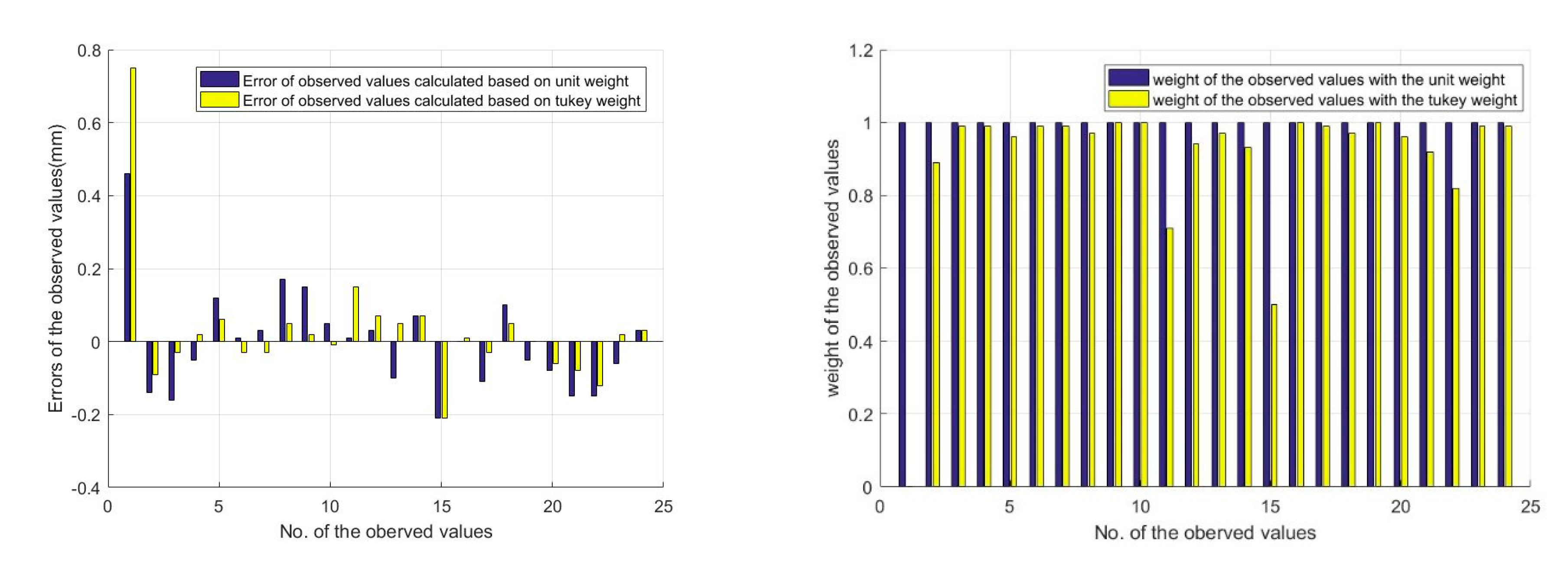
Figure 10 show the residual errors and the weights of group 1 calculated by this paper’s two methods. The residual errors vary in size and distribution. Some are less than the m0, some are in the range of 1–2 times, and some are more than two times. When using the unit weight method for calculations, the weight of each observation value is one. In this case, the observations cannot be treated differently. When the Tukey weight method is used for calculations, however, the weights of the observed values are different depending on the residual value. In this case, the contribution of the observation values to the results can be changed, and the contribution of harmful observation values can be reduced or even suppressed. For example, the error of observation is 0.75 mm—more than three times m0—and its weight is zero.

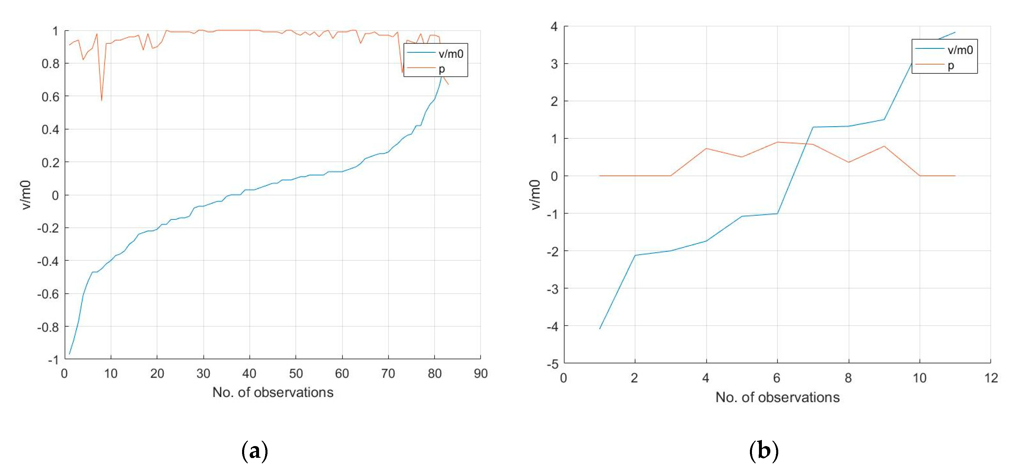
In order to illustrate the weights of the observed values, Figure 11 shows the corresponding relationship between the residual error and the weight. The blue line represents the ratio between the residual error (listed as v) and the m0, and the red line represents the weight value. Figure 11a shows the weight of the observation value when v is less than m0, and the weight decreases with an increase in the gross error; the maximum weight is 1.00, and the minimum weight is 0.57. Figure 11b shows the weight of the observation value when the error is greater than m0. The results show that the greater the gross errors, the smaller the weights. For instance, the weights of the observations with errors in the range of 1–2 times the m0 have a minimum of 0.36 and a maximum of 0.90, while observations with errors more than twice the m0 are harmful, and their weights are zero.

In this paper, the positions of the platform calculated by the two methods are compared with the actual positions collected by the electronic total station, and the accuracy is able to reach the millimetre level. The results are shown in

Table 2. The results and errors of the spatial positions.

Group	Results	X [mm]	Y [mm]	Z [mm]	ex [mm]	ey [mm]	ez [mm]
1	Method1	6932.40	9410.20	12062.00	−78.60	−23.80	48.00
	Method2	6957.00	9416.00	12048.00	−54.00	−18.00	34.00
	True value	7011.00	9434.00	12014.00	exy increase 30.69%		ez increase 29.17%
2	Method1	6991.10	9246.10	12189.00	79.10	−28.90	−12.00
	Method2	6876.00	9235.90	12206.00	−36.00	−39.10	5.00
	True value	6912.00	9275.00	12201.00	exy increase 36.89%		ez increase 58.33%
3	Method1	7436.20	9432.00	12041.00	−9.80	−37.00	−27.00
	Method2	7435.10	9485.00	12075.00	−10.90	16.00	7.00
	True value	7446.00	9469.00	12068.00	exy increase 49.42%		ez increase 74.07%
4	Method1	8506.30	9533.40	15264.00	90.30	−52.60	16.00
	Method2	8342.60	9612.50	15242.00	−73.40	26.50	−6.00
	True value	8416.00	9586.00	15248.00	exy increase 29.76%		ez increase 62.50%

.

Using the experimental conditions of monocular vision, the position precision calculated by the Tukey weight method was improved compared to the unit weight method. The precision of the plane minimum increased by 29.76%, and the maximum increased by 49.42%, while the precision of the elevation minimum increased by 29.17%, and the maximum increased by 74.07%.

According to the experiments, the results show that the gross errors of the observations can be detected effectively with the Tukey weight method. Additionally, the observations with different sizes of gross errors will have an optimal value, and the accuracy of the measurement results will be improved.

3.2. Experiment 2

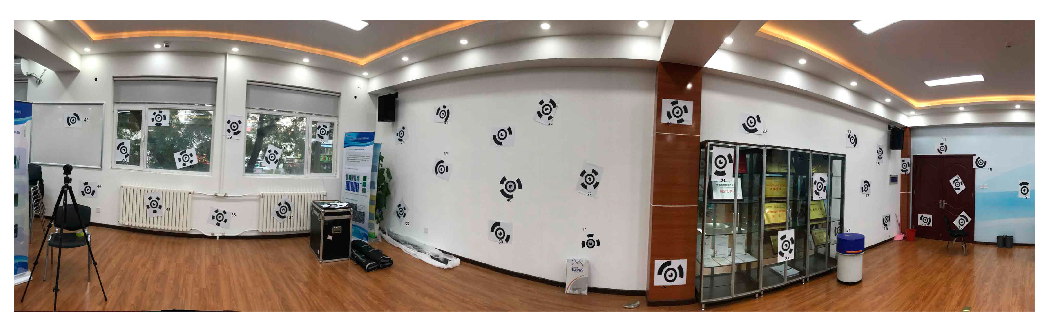
In this experiment, a ‘u’ type indoor wall with 39 coding graphics was chosen as the experimental environment, as shown in Figure 12. The coding images were automatically acquired from 12 different stations when the platform was moving. Each coding image included five to eight coding graphics. The calculation results for the positions of the platform were then compared.

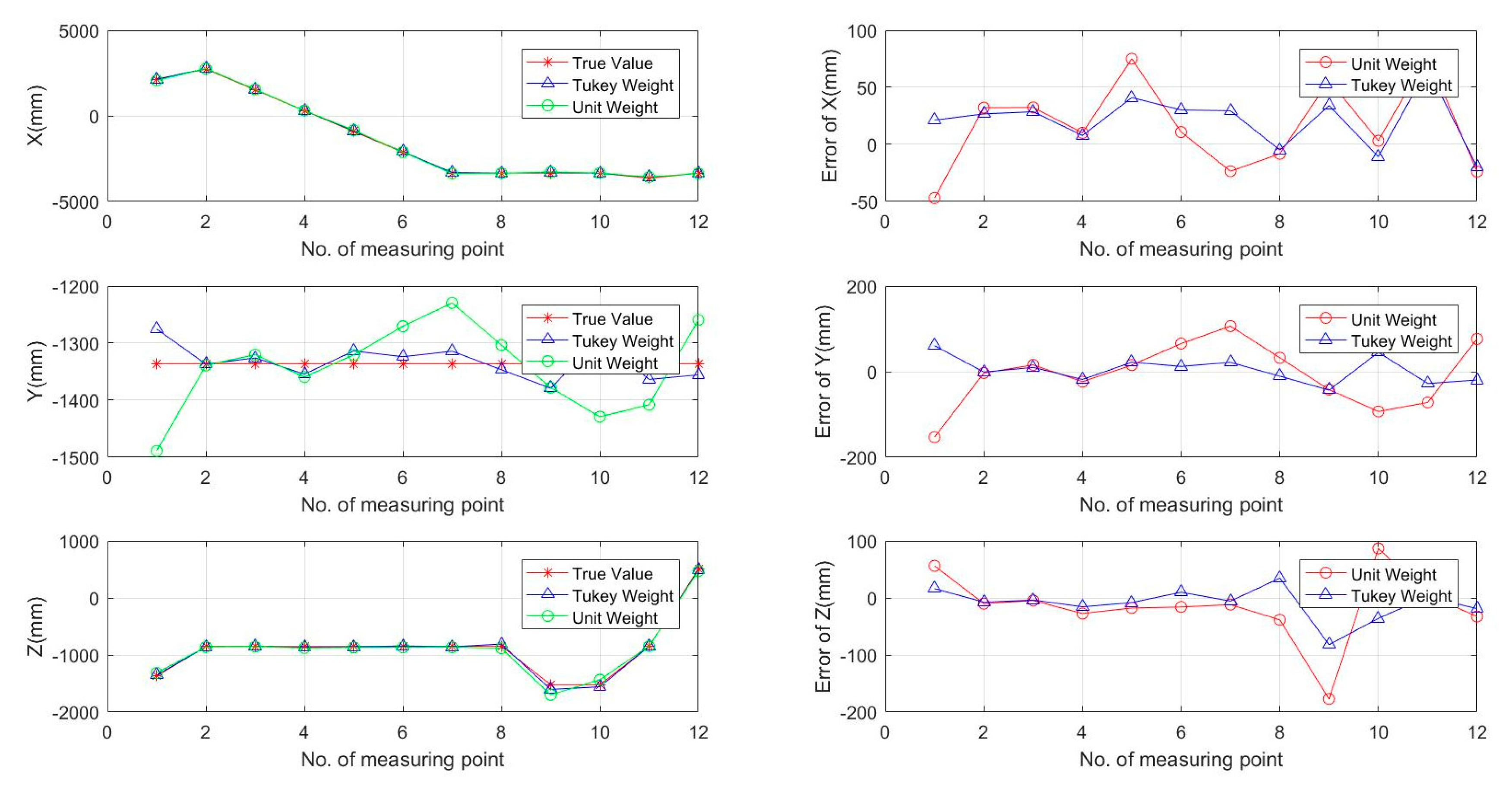
In the experiments, the positions of the platform obtained by the electronic total station were regarded as the true values, and the accuracy was able to reach the millimetre level. The results that were calculated by the two methods of this paper were compared. Figure 13 shows the three axial variations in X, Y, and Z in the O–XYZ stereo space, as well as a trajectory accuracy comparison between the two methods.

It can be seen from the diagram that, compared to the unit weight method, the results calculated by the Tukey weight method are closer to the true value, and the error value is smaller; thus, the accuracy is improved. The results of the calculations of the two methods are shown in

Table 3. Results of experiment 2.

Station	Results	X [mm]	Y [mm]	Z [mm]	Accuracy Improvement in Plane	Accuracy Improvement in Elevation
1	Method1	2073.00	−1489.00	−1313.70	Increase 59.81%	Increase 71.05%
	Method2	2141.30	−1275.30	−1353.70
	True value	2120.00	−1336.00	−1370.00
2	Method1	2767.20	−1339.00	−860.03	Increase 17.40%	Increase 25.98%
	Method2	2761.70	−1336.80	−857.42
	True value	2735.00	−1336.00	−850.00
3	Method1	1550.40	−1320.10	−854.52	Increase 15.96%	Increase 18.446%
	Method2	1546.60	−1325.90	−853.69
	True value	1518.00	−1336.00	−850.00
4	Method1	310.14	−1359.40	−877.33	Increase 21.97%	Increase 43.55%
	Method2	307.82	−1354.30	−865.42
	True value	300.00	−1336.00	−850.00
5	Method1	−835.93	−1320.50	−867.53	Increase 39.08%	Increase 53.26%
	Method2	−869.97	−1313.70	−858.19
	True value	−911.00	−1336.00	−850.00
6	Method1	−2115.20	−1270.30	−865.79	Increase 51.02%	Increase 36.424%
	Method2	−2095.80	−1323.70	−839.96
	True value	−2126.00	−1336.00	−850.00
7	Method1	−3364.50	−1229.40	−861.68	Increase 66.34%	Increase 52.13%
	Method2	−3311.50	−1314.10	−855.59
	True value	−3341.00	−1336.00	−850.00
8	Method1	−3348.20	−1303.40	−881.37	Increase 65.53%	Increase 9.40%
	Method2	−3344.90	−1346.50	−808.24
	True value	−3340.00	−1336.00	−843.00
9	Method1	−3283.90	−1378.00	−1699.10	Increase 21.78%	Increase 53.75%
	Method2	−3306.00	−1379.00	−1603.90
	True value	−3340.00	−1336.00	−1522.00
10	Method1	−3336.80	−1429.00	−1435.10	Increase 50.03%	Increase 58.80%
	Method2	−3350.90	−1290.80	−1557.80
	True value	−3340.00	−1336.00	−1522.00
11	Method1	−3567.90	−1407.90	−844.55	Increase 31.74%	Increase 58.88%
	Method2	−3579.00	−1363.60	−847.76
	True value	−3646.00	−1336.00	−850.00
12	Method1	−3363.80	−1259.40	471.51	Increase 65.35%	Increase 42.39%
	Method2	−3359.80	−1355.50	485.28
	True value	−3340.00	−1336.00	504.00

.

Using the experimental conditions of monocular vision, the position precision calculated by the Tukey weight method was improved more significantly than the unit weight method. The precision of the plane minimum was increased by 16.96%, and the maximum increased by 66.34%, while the precision of the elevation minimum increased by 9.40%, and the maximum increased by 71.05%.

3.3. Experiment 3

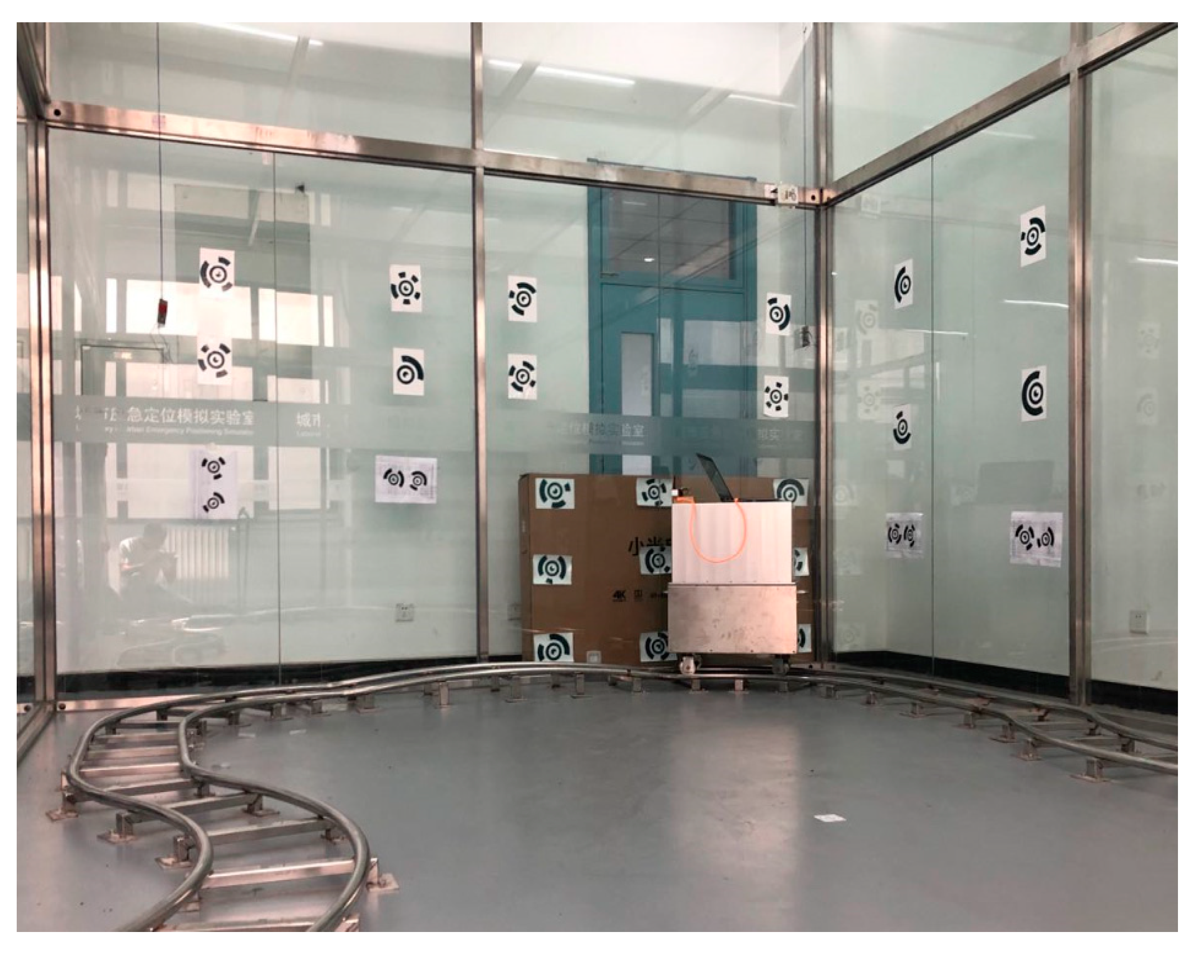
In order to verify the accuracy of the proposed method, an experiment was carried out in the indoor navigation and positioning laboratory of a university, as shown in Figure 14. The laboratory has a fixed orbit with known spatial information, and the accuracy was able to reach the millimetre level. This laboratory also features an electrically driven autonomous rail vehicle. During the experiment, the camera was installed in a rail car that moved along a fixed route, and the images were collected.

During the course of the experiment, a total of 51 images were obtained. Using this paper’s method, the position of the vehicle when taking pictures was calculated, and the running track of the vehicle was drawn, as shown in Figure 15.

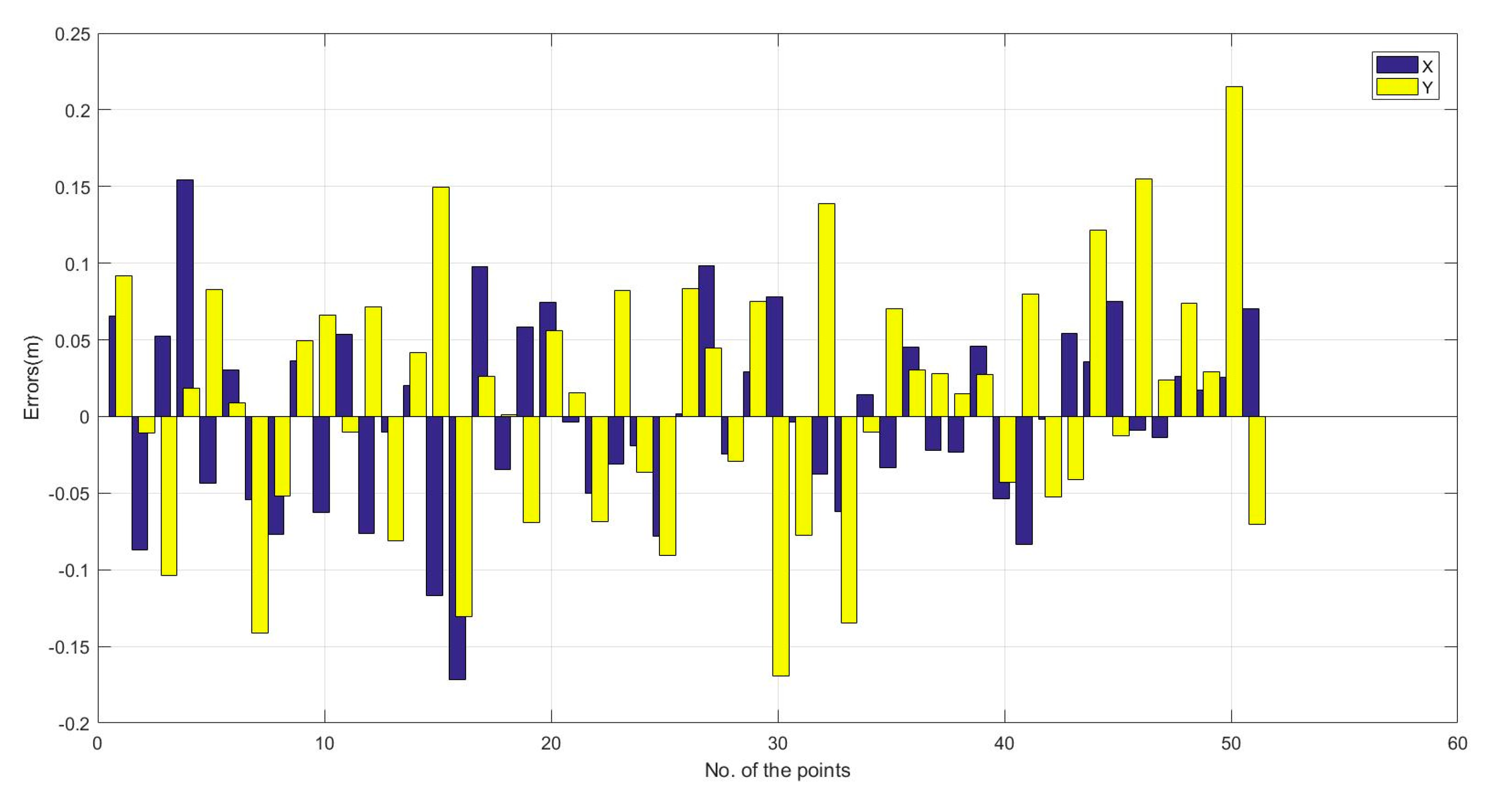
By comparing the vehicle position calculated by this method with the nearest point on the track, the plane position measurement deviation of this method was obtained, as shown in Figure 16. The maximum measurement deviation was 0.17 m in the X direction and 0.22 m in the Y direction. The plane RMSE was 0.14 m.

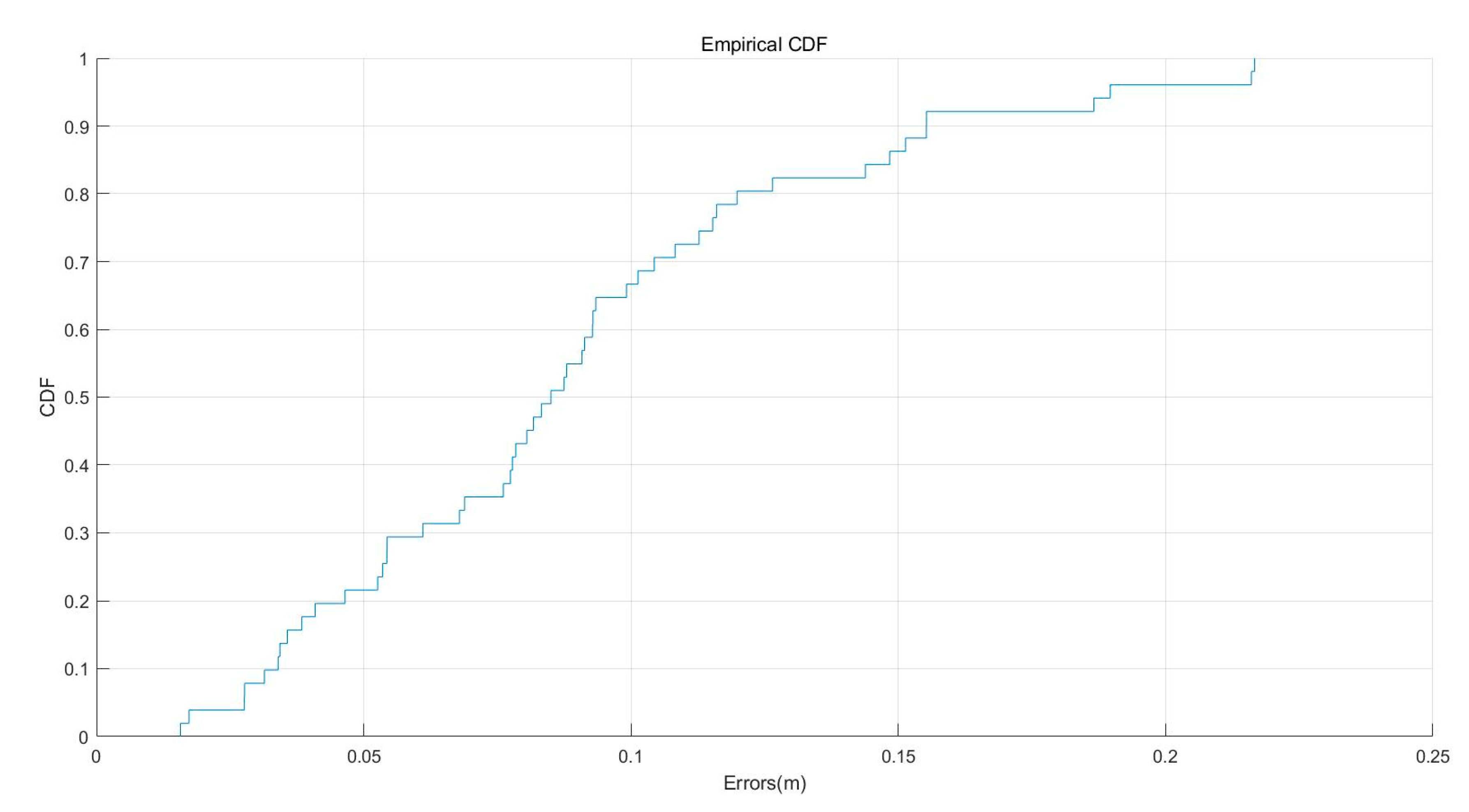
Figure 17 shows the cumulative distribution function (CDF) curve of the error, showing the distribution range of the error. It can be seen that about 22% of the points has a positioning accuracy better than 0.05 m, about 67% of the points had a positioning accuracy better than 0.1 m, about 96% of the points had a positioning accuracy better than 0.15 m, and only about 4% of the points had an error between 0.2 and 0.25 m.

Based on a study of the full text, we can see that using vision sensors as a streaming media technology can not only achieve rich environmental information but can also be transmitted in real time. In terms of visual positioning, the mainstream technical methods include SLAM, VO, image fingerprinting-based methods, and integrated external sensor methods. SLAM and VO achieve relative positioning without the assistance of external information. The proposed method in this paper achieved absolute positioning and can be used as an auxiliary measure of the former methods to achieve the absolute positioning of large scenes. Compared with image fingerprinting-based methods, our method is a special case, as it does not need to build an image database of all indoor environments and can also be used as a control measurement method. Compared with sensor-assisted positioning methods such as UWB, this paper’s method relies solely on visual positioning to achieve equivalent or higher precision positioning results, which gives it an advantage. However, this method also has some shortcomings, such as the need to deploy coding graphics and measure the coordinates in advance, which requires some preparatory work, especially when applied to a large-scale environment. At the same time, due to the limitations of feature extraction and other technologies, location failures can easily occur in areas where texture is sparse or the light intensity changes rapidly. For this reason, the fusion of this method with SLAM, VO, and/or multi-sensor methods may give it better application potential.

4. Conclusions and Outlook

This paper adopted the combined methods of coding graphics and monocular vision, which can automatically obtain an observed image’s coordinates and the world coordinates of the center of the coding graphics. The two methods (based on unit weight and Tukey weight, respectively) developed in this paper can be used to calculate the position of mobile platforms in a room with good accuracy. The Tukey weight method can identify the gross errors in observations effectively and calculate the weight of the observations according to their gross errors. Additionally, this method can optimize the participation of observation values through the weight size and enhance the accuracy of the results. Based on the results of these experiments, the plane precision increased by an average of 39.43%, and the elevation accuracy increased by an average of 49.85%. These results show that this method is feasible and can thus improve the accuracy of the indoor positioning measurements of a mobile platform. In addition, the research results of this paper can be used as the absolute positioning benchmark for SLAM and VO technology, which can achieve absolute positioning and, with the help of natural features, will greatly reduce the preparation of coded graphics. Moreover, by solving the positioning problem, we can obtain environmental information in real time, which can facilitate the emergency rescue of indoor and underground spaces and three-dimensional real-scene data collection.

However, in order to solve the visual positioning failures caused by sparse texture, light changes, and other factors, the indoor positioning method proposed in this paper can be integrated into the Inertial Navigation System (INS) and wireless signal-based solutions in the future. In doing so, this method can provide continuous indoor and outdoor unified localization and navigation.

References

- Ruizhi, C. Mobile phone thinking engine leads intelligent location service. J. Navig. Position. 2017, 5, 1–3. [Google Scholar]
- China Earth Observation and Navigation Technology Field Navigation Expert Group. Indoor and Outdoor High Accuracy Positioning and Navigation White Paper; Ministry of Science and Technology of the People’s Republic of China: Beijing, China, 2013; pp. 6–10.
- Abdulrahman, A.; AbdulMalik, A.-S.; Mansour, A.; Ahmad, A.; Suheer, A.-H.; Mai, A.-A.; Hend, A.-K. Ultra Wideband Indoor Positioning Technologies: Analysis and Recent Advances. Sensors 2016, 16, 707. [Google Scholar]
- Liu, F.; Wang, J.; Zhang, J.X.; Han, H. An Indoor Localization Method for Pedestrians Base on Combined UWB/PDR/Floor Map. Sensors 2019, 19, 2578. [Google Scholar] [CrossRef] [PubMed] [Green Version]
- Stella, M.; Russo, M.; Begušić, D. RF Localization in Indoor Environment. Radioengineering 2012, 21, 557–567. [Google Scholar]
- Kim, Y.-G.; An, J.; Lee, K.-D. Localization of Mobile Robot Based on Fusion of Artificial Landmark and RF TDOA Distance under Indoor Sensor Network. Int. J. Adv. Robot. Syst. 2011, 8, 52. [Google Scholar] [CrossRef] [Green Version]
- Chen, Z.; Zou, H.; Jiang, H.; Zhu, Q.; Soh, Y.C.; Xie, L. Fusion of WiFi, Smartphone Sensors and Landmarks Using the Kalman Filter for Indoor Localization. Sensors 2015, 15, 715–732. [Google Scholar] [CrossRef]
- Trawinski, K.; Alonso, J.M.; Hernández, N. A multiclassifier approach for topology-based WiFi indoor localization. Soft Comput. 2013, 17, 1817–1831. [Google Scholar] [CrossRef]
- Kriz, P.; Maly, F.; Kozel, T. Improving Indoor Localization Using Bluetooth Low Energy Beacons. Mob. Inf. Syst. 2016, 2016, 1–11. [Google Scholar] [CrossRef] [Green Version]
- Patil, A.; Kim, D.J.; Ni, L.M. A study of frequency interference and indoor location sensing with 802.11b and Bluetooth technologies. Int. J. Mob. Commun. 2006, 4, 621. [Google Scholar] [CrossRef]
- Piciarelli, C. Visual Indoor Localization in Known Environments. IEEE Signal Process. Lett. 2016, 23, 1330–1334. [Google Scholar] [CrossRef]
- Feng, G.; Ma, L.; Tan, X. Visual Map Construction Using RGB-D Sensors for Image-Based Localization in Indoor Environments. J. Sens. 2017, 2017, 1–18. [Google Scholar] [CrossRef] [Green Version]
- Luoh, L. ZigBee-based intelligent indoor positioning system soft computing. Soft Comput. 2013, 18, 443–456. [Google Scholar] [CrossRef]
- Niu, J.; Wang, B.; Shu, L.; Duong, T.Q.; Chen, Y. ZIL: An Energy-Efficient Indoor Localization System Using ZigBee radio to Detect WiFi Fingerprints. IEEE J. Sel. Areas Commun. 2015, 33, 1. [Google Scholar] [CrossRef] [Green Version]
- Marín, L.; Vallés, M.; Soriano, Á.; Valera, A.; Albertos, P. Multi Sensor Fusion Framework for Indoor-Outdoor Localization of Limited Resource Mobile Robots. Sensors 2013, 13, 14133–14160. [Google Scholar] [CrossRef] [PubMed]
- Xiao, J.; Zhou, Z.; Yi, Y.; Ni, L.M. A Survey on Wireless Indoor Localization from the Device Perspective. ACM Comput. Surv. 2016, 49, 1–31. [Google Scholar] [CrossRef]
- Wang, B.; Zhou, J.; Tang, G.; Di, K.; Wan, W.; Liu, C.; Wang, J. Research on visual localization method of lunar rover. Sci. Sin. Inf. 2014, 44, 452–460. [Google Scholar]
- Di, K. A Review of Spirit and Opportunity Rover Localization Methods. Spacecr. Eng. 2009, 5, 1–5. [Google Scholar]
- Scaramuzza, D.; Fraundorfer, F. Visual odometry Part I: The First 30 Years and Fundamentals. IEEE Robot. Autom. Mag. 2011, 18, 80–92. [Google Scholar] [CrossRef]
- Sadeghi, H.; Valaee, S.; Shirani, S.; Sadeghi, H. A weighted KNN epipolar geometry-based approach for vision-based indoor localization using smartphone cameras. In Proceedings of the 2014 IEEE 8th Sensor Array and Multichannel Signal Processing Workshop (SAM), A Coruna, Spain, 22–25 June 2014; pp. 37–40. [Google Scholar]
- Treuillet, S.; Royer, E. Outdoor/indoor vision-based localization for blind pedestrian navigation assistance. Int. J. Image Graph. 2010, 10, 481–496. [Google Scholar] [CrossRef] [Green Version]
- Elloumi, W.; Latoui, A.; Canals, R.; Chetouani, A.; Treuillet, S. Indoor Pedestrian Localization with a Smartphone: A Comparison of Inertial and Vision-based Methods. IEEE Sens. J. 2016, 16, 1. [Google Scholar] [CrossRef]
- Vedadi, F.; Valaee, S. Automatic Visual Fingerprinting for Indoor Image-Based Localization Applications. IEEE Trans. Syst. Man Cybern. Syst. 2020, 50, 305–317. [Google Scholar] [CrossRef]
- Liang, J.Z.; Corso, N.; Turner, E.; Zakhor, A. Image Based Localization in Indoor Environments. In Proceedings of the 2013 Fourth International Conference on Computing for Geospatial Research and Application, San Jose, CA, USA, 22–24 July 2013; Institute of Electrical and Electronics Engineers (IEEE): San Jose, CA, USA, 2013; pp. 70–75. [Google Scholar]
- Royer, E.; Lhuillier, M.; Dhome, M.; Lavest, J.-M. Monocular Vision for Mobile Robot Localization and Autonomous Navigation. Int. J. Comput. Vis. 2007, 74, 237–260. [Google Scholar] [CrossRef] [Green Version]
- Mur-Artal, R.; Montiel, J.M.M.; Tardos, J. ORB-SLAM: A Versatile and Accurate Monocular SLAM System. IEEE Trans. Robot. 2015, 31, 1147–1163. [Google Scholar] [CrossRef] [Green Version]
- Zou, X.; Zou, H.; Lu, J. Virtual manipulator-based binocular stereo vision positioning system and errors modelling. Mach. Vis. Appl. 2010, 23, 43–63. [Google Scholar] [CrossRef]
- Domingo, J.D.; Cerrada, C.; Valero, E.; Cerrada, J. An Improved Indoor Positioning System Using RGB-D Cameras and Wireless Networks for Use in Complex Environments. Sensors 2017, 17, 2391. [Google Scholar] [CrossRef] [Green Version]
- Liu, Z.; Jiang, N.; Zhang, L. Self-localization of indoor mobile robots based on artificial landmarks and binocular stereo vision. In Proceedings of the 2009 International Workshop on Information Security and Application (IWISA 2009), Qingdao, China, 21–22 November 2009; p. 338. [Google Scholar]
- Zhong, X.; Zhou, Y.; Liu, H. Design and recognition of artificial landmarks for reliable indoor self-localization of mobile robots. Int. J. Adv. Robot. Syst. 2017, 14, 1729881417693489. [Google Scholar] [CrossRef] [Green Version]
- Xiao, A.; Chen, R.; Li, D.R.; Chen, Y.; Wu, D. An Indoor Positioning System Based on Static Objects in Large Indoor Scenes by Using Smartphone Cameras. Sensors 2018, 18, 2229. [Google Scholar] [CrossRef] [Green Version]
- Ramirez, B.; Chung, H.; Derhamy, H.; Eliasson, J.; Barca, J.C. Relative localization with computer vision and UWB range for flying robot formation control. In Proceedings of the 2016 14th International Conference on Control, Automation, Robotics and Vision (ICARCV), Phuket, Thailand, 13–15 November 2016; Institute of Electrical and Electronics Engineers (IEEE): Phuket, Thailand, 2016; pp. 1–6. [Google Scholar]
- Tiemann, J.; Ramsey, A.; Wietfeld, C. Enhanced UAV Indoor Navigation through SLAM-Augmented UWB Localization. In Proceedings of the 2018 IEEE International Conference on Communications Workshops (ICC Workshops), Kansas City, MO, USA, 20–24 May 2018; pp. 1–6. [Google Scholar]
- Muñoz-Salinas, R.; Marin-Jimenez, M.J.; Yeguas, E.; Medina-Carnicer, R. Mapping and localization from planar markers. Pattern Recognit. 2018, 73, 158–171. [Google Scholar] [CrossRef] [Green Version]
- Lim, H.; Lee, Y.S. Real-Time Single Camera SLAM Using Fiducial Markers. In Proceedings of the ICCAS-SICE, Fukuoka City, Japan, 18–21 August 2009. [Google Scholar]
- Fraundorfer, F.; Scaramuzza, D. Visual Odometry: Part II: Matching, Robustness, Optimization, and Applications. IEEE Robot. Autom. Mag. 2012, 19, 78–90. [Google Scholar] [CrossRef] [Green Version]
- Zhou, J.; Huang, Y.; Yang, Y.; Ou, J. Robust Least Square Method; Huazhong University of Science and Technology Press: Wuhan, China, 1991. [Google Scholar]
- Tukey, J.W. Study of Robustness by Simulation: Particularly Improvement by Adjustment and Combination. In Robustness in Statistics; Academic Press: New York, NY, USA, 1979; pp. 75–102. [Google Scholar]
- Kafadar, K. John Tukey and Robustness. Stat. Sci. 2003, 18, 319–331. [Google Scholar] [CrossRef]
- Huber, P.J.; John, W. Tukey’s Contributions to Robust Statistics. Ann. Stat. 2002, 30, 1640–1648. [Google Scholar]
- Wang, Z.; Wu, L.-X.; Li, H.-Y. Key technology of mine underground mobile positioning based on LiDAR and coded sequence pattern. Trans. Nonferrous Met. Soc. China 2011, 21, s570–s576. [Google Scholar] [CrossRef]
- Gary, B.; Adrian, K. Learning OpenCV3, 3rd ed.; O’Reilly Media, Inc.: Sebastopol, CA, USA, 2016. [Google Scholar]
- Willian, K.P. Digital Image Processing, 3rd ed.; John Wiley & Sons, Inc.: Hoboken, NJ, USA, 2001. [Google Scholar]
- Otsu, N. A Threshold Selection Method from Gray-Level Histograms. IEEE Trans. Syst. Man, Cybern. 1979, 9, 62–66. [Google Scholar] [CrossRef] [Green Version]
- Hu, W.; Li, C.C.; Dai, G.H. Reform Based on “No Paper-Drawing” Mechanical Drawing Course System. Adv. Mater. Res. 2011, 271, 1519–1523. [Google Scholar] [CrossRef]
- Liao, X.; Feng, W. Determination of the Deviation between the Image of a Circular Target Center and the Center of the Ellipse in the Image. J. Wuhan Tech. Univ. Surv. 1999, 24, 235–239. [Google Scholar]
- Zhang, J.Q.; Pan, L.; Wang, S.G. Photogrammetry; Wuhan University Press: Wuhan, China, 2008. [Google Scholar]
- Zhang, Z. A flexible new technique for camera calibration. IEEE Trans. Pattern Anal. Mach. Intell. 2000, 22, 1330–1334. [Google Scholar] [CrossRef] [Green Version]
Figure 1.
Technical flowchart.
Figure 2.
(a) The coding graphic example. (b) The template graphic.
Figure 3.
Flowchart of coding graphics identification and localization.
Figure 4.
Coding Image.
Figure 5.
Contour Matching Results.
Figure 6.
Interference Contour Culling Results.
Figure 7.
Coding graphic centroid.
Figure 8.
The functions of Tukey.
Figure 9.
Experiment images. (a–d) show the images from group 1 to group 4.
Figure 10.
Error and weight of the observation values.
Figure 11.
(a) Relationships between v/m0 and weight P, with v less than m0. (b) Relationships between v/m0 and weight P, with v greater than m0.
Figure 12.
A panoramic photo of the environment of experiment 3.
Figure 13.
The moving trajectory of the platform and the accuracy comparison between the two methods.
Figure 14.
Experimental environment.
Figure 15.
The vehicle trajectory calculated by the Tukey weight method.
Figure 16.
Difference between the coordinates of the orbit and the calculation results.
Figure 17.
The cumulative distribution function (CDF) curve of the residual errors.