Land Use and Land Cover Change Modeling and Future Potential Landscape Risk Assessment Using Markov-CA Model and Analytical Hierarchy Process

 , , ,
, , ,  and
and
Abstract
:1. Introduction
2. Materials and Methods
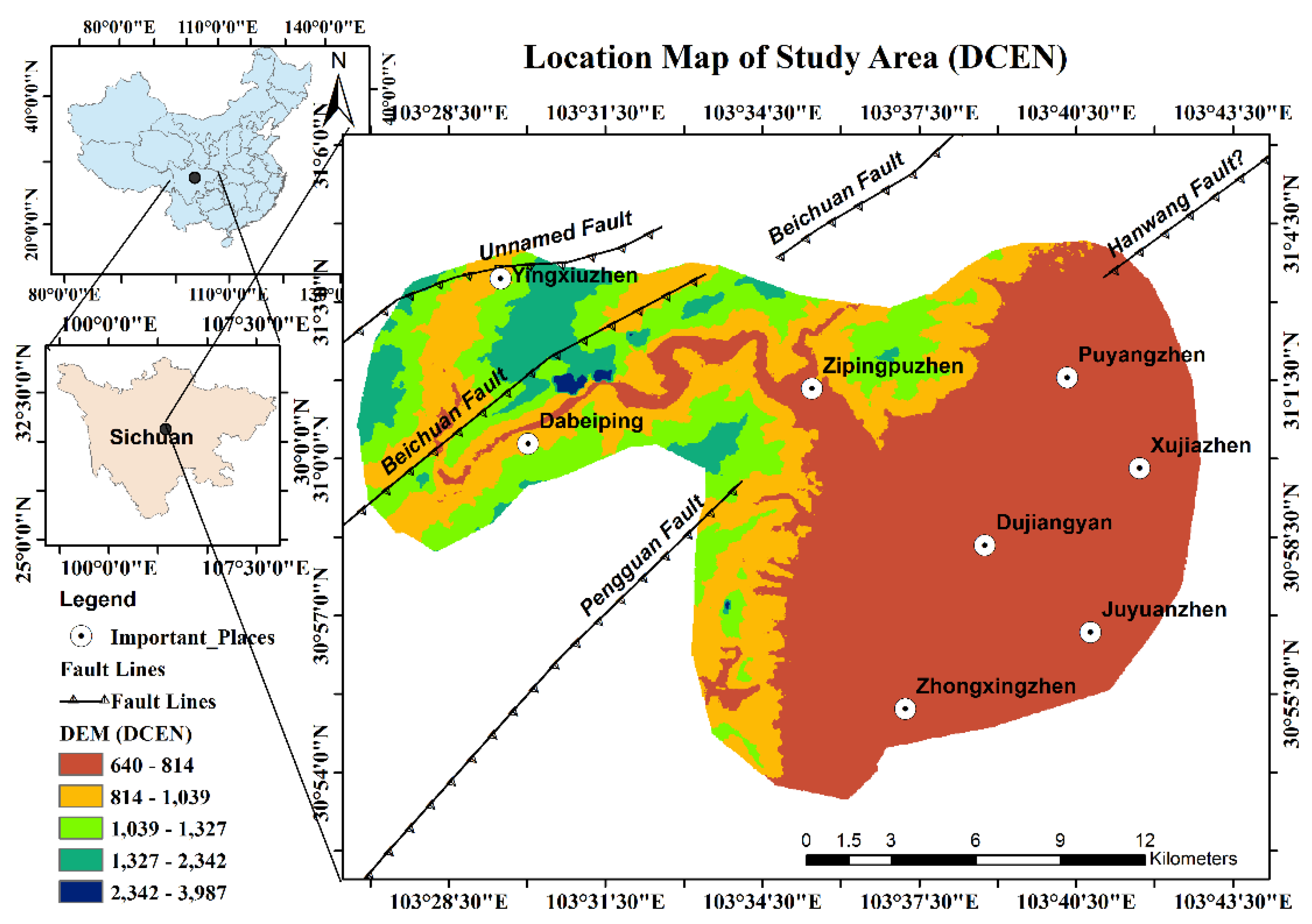
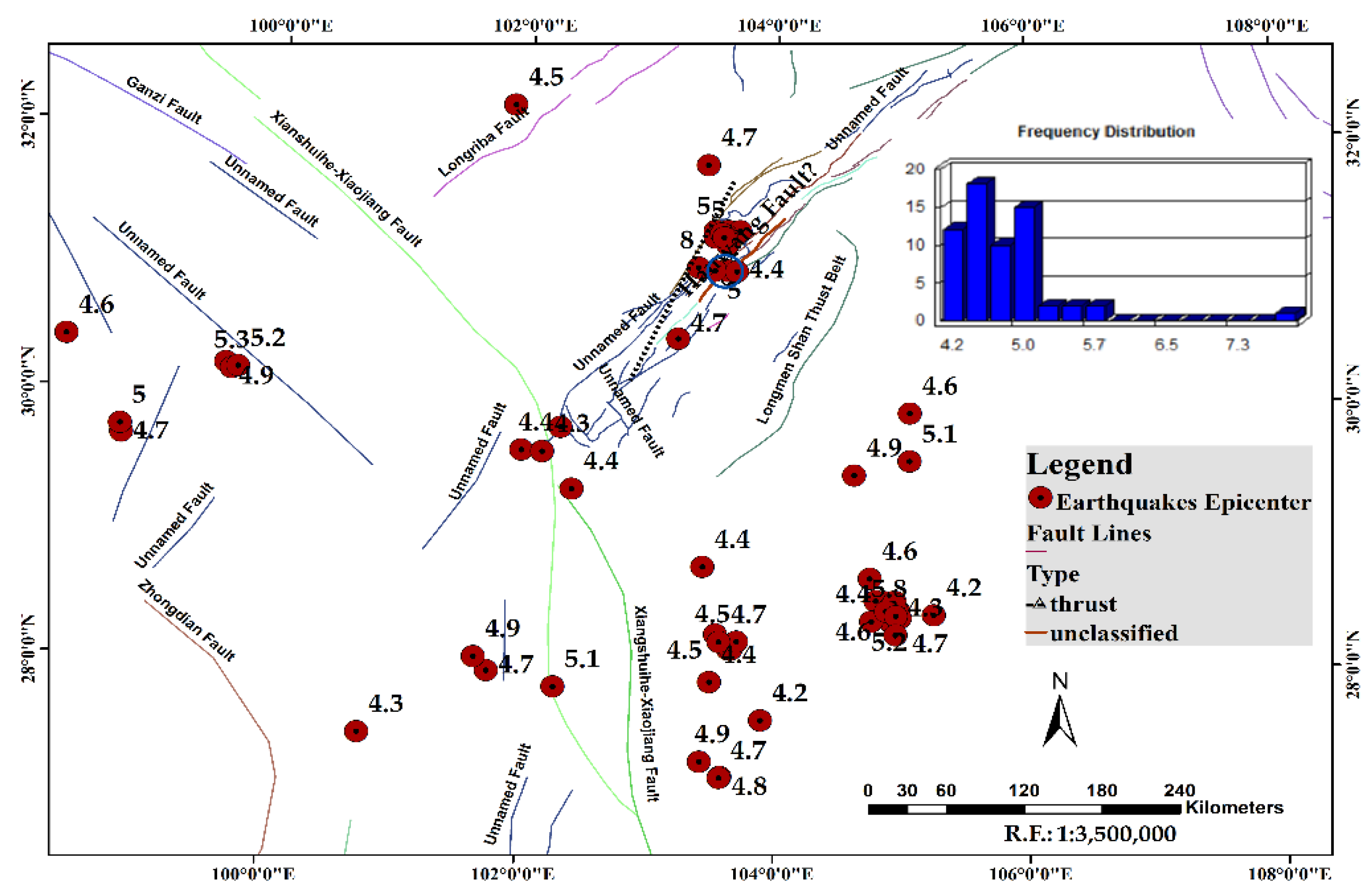
2.1. Study Area
2.2. Data
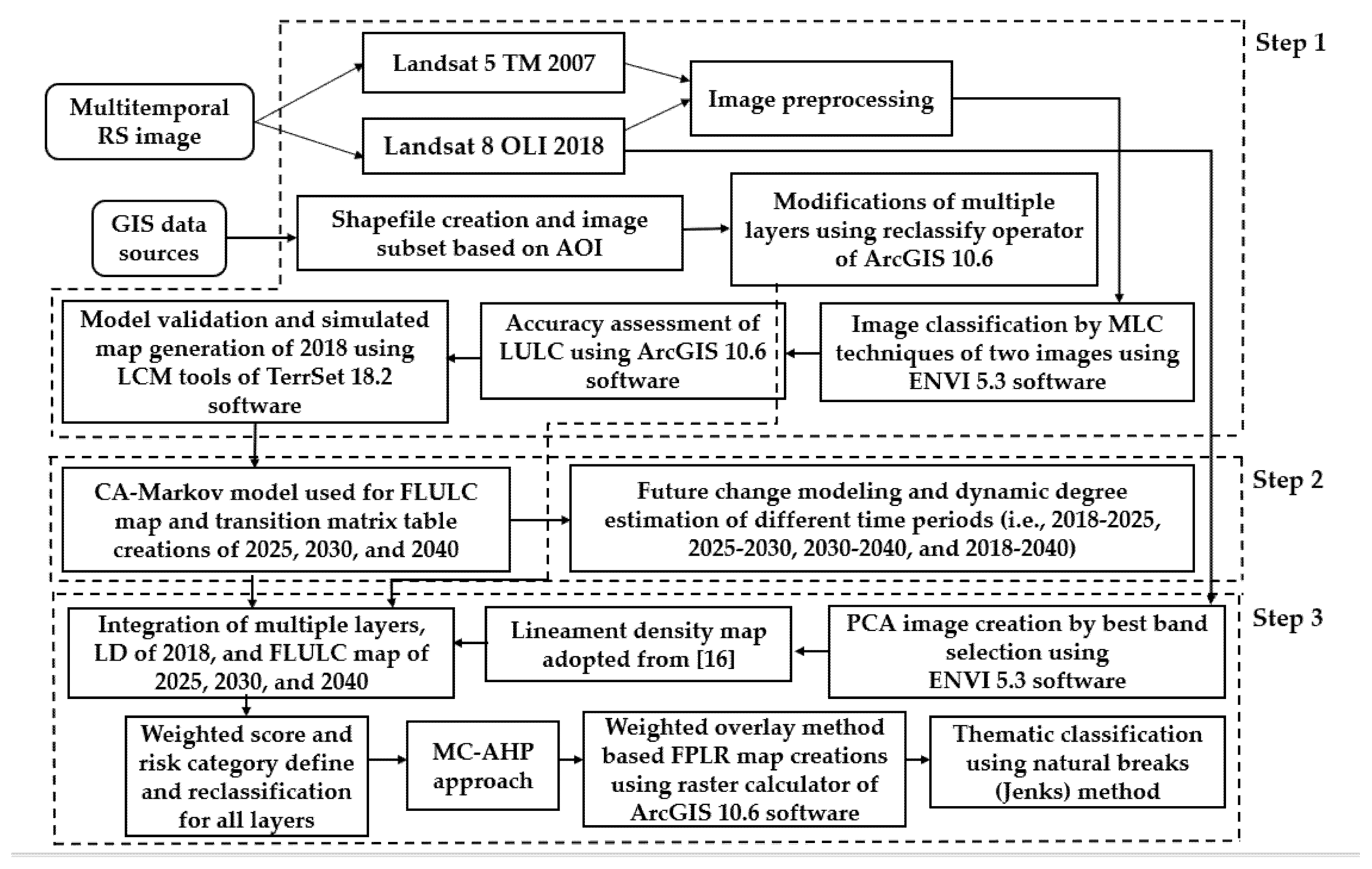
2.3. Methodology
2.3.1. LULCC Modeling Using Land Change Modeler
2.3.2. FLULC Dynamic Degree Estimation and Transition Matrices Computation Method
2.3.3. FPLR Evaluation Method
3. Results
3.1. Validation of Future LULCC Prediction
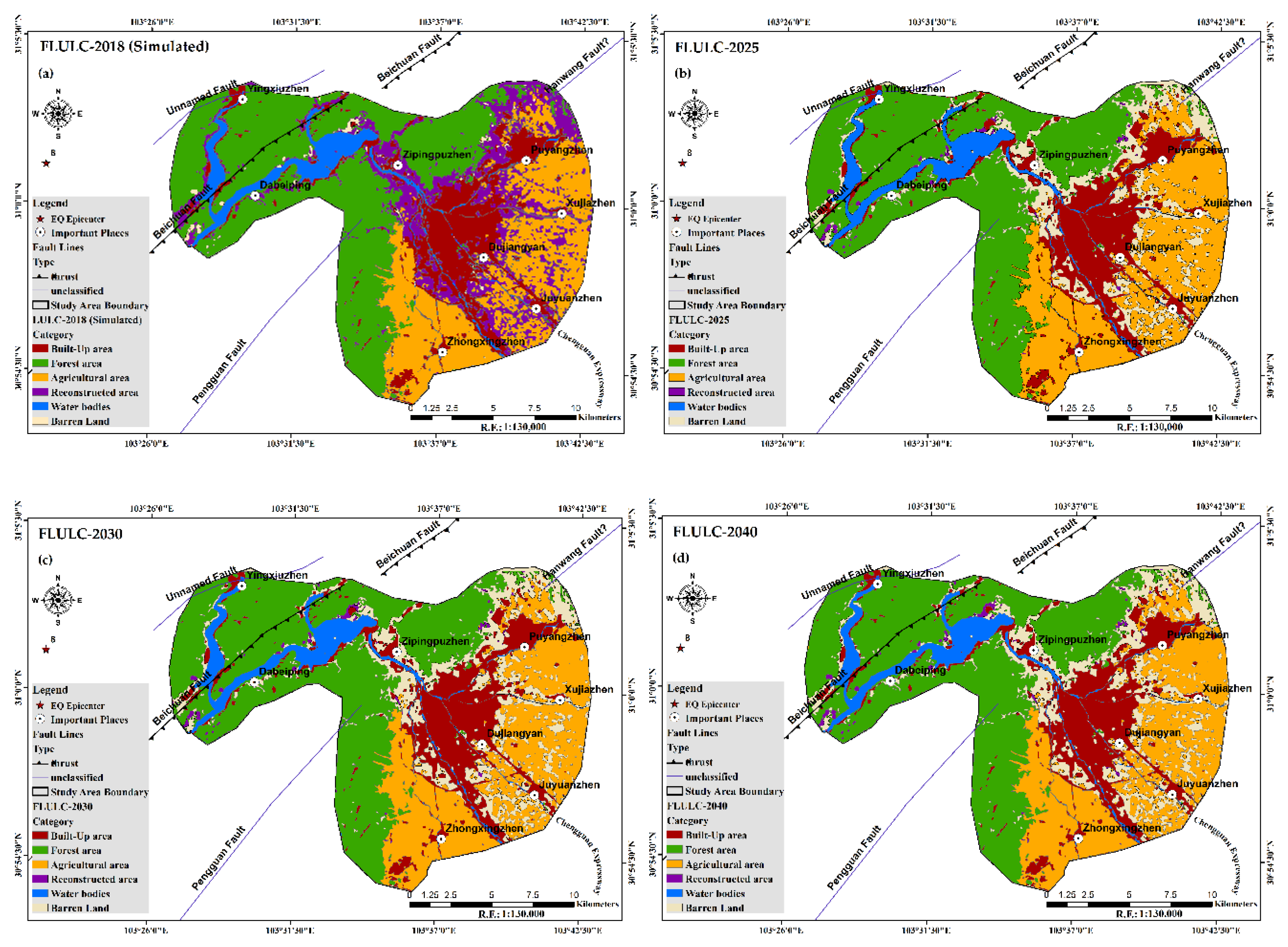
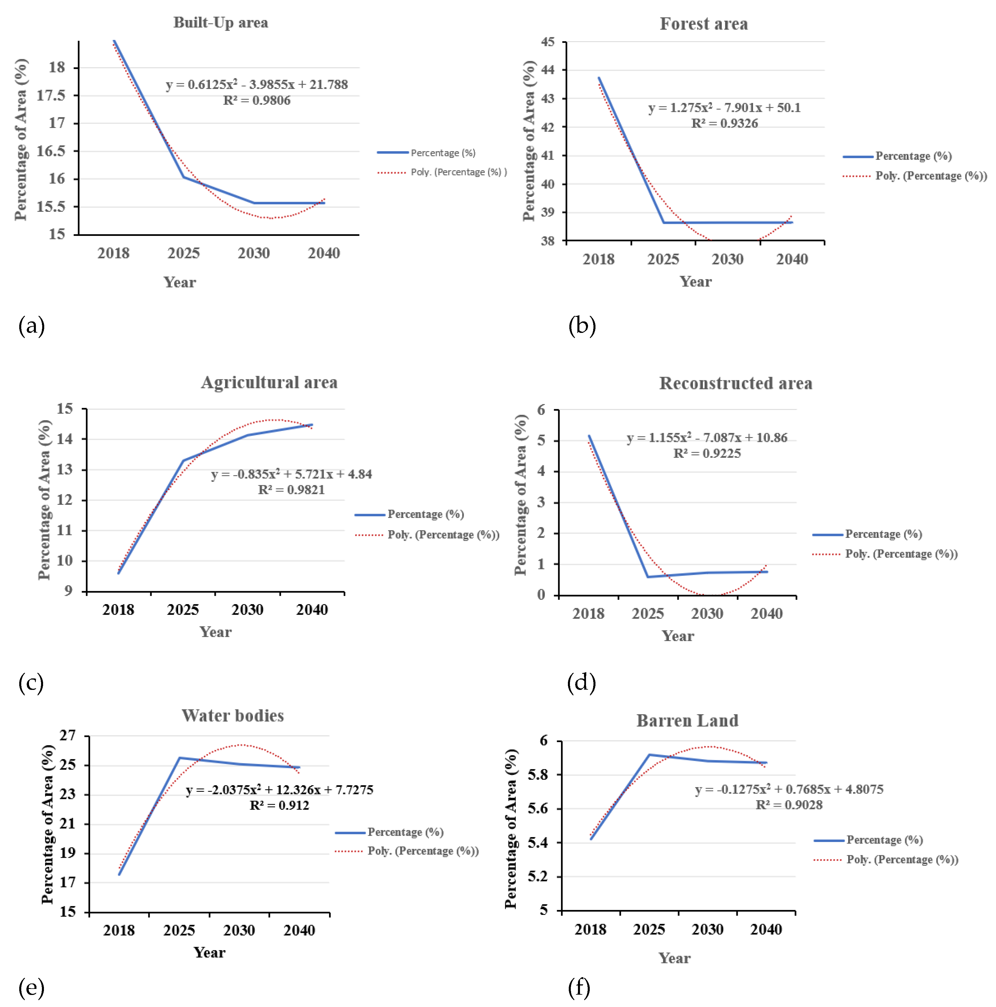
3.2. FLULC Change, Dynamic Degree and Gain and Loss Estimation based on 2018–2040 data
3.3. Analysis of FLULC Transition Probability Matrix (TPM) by Percentage
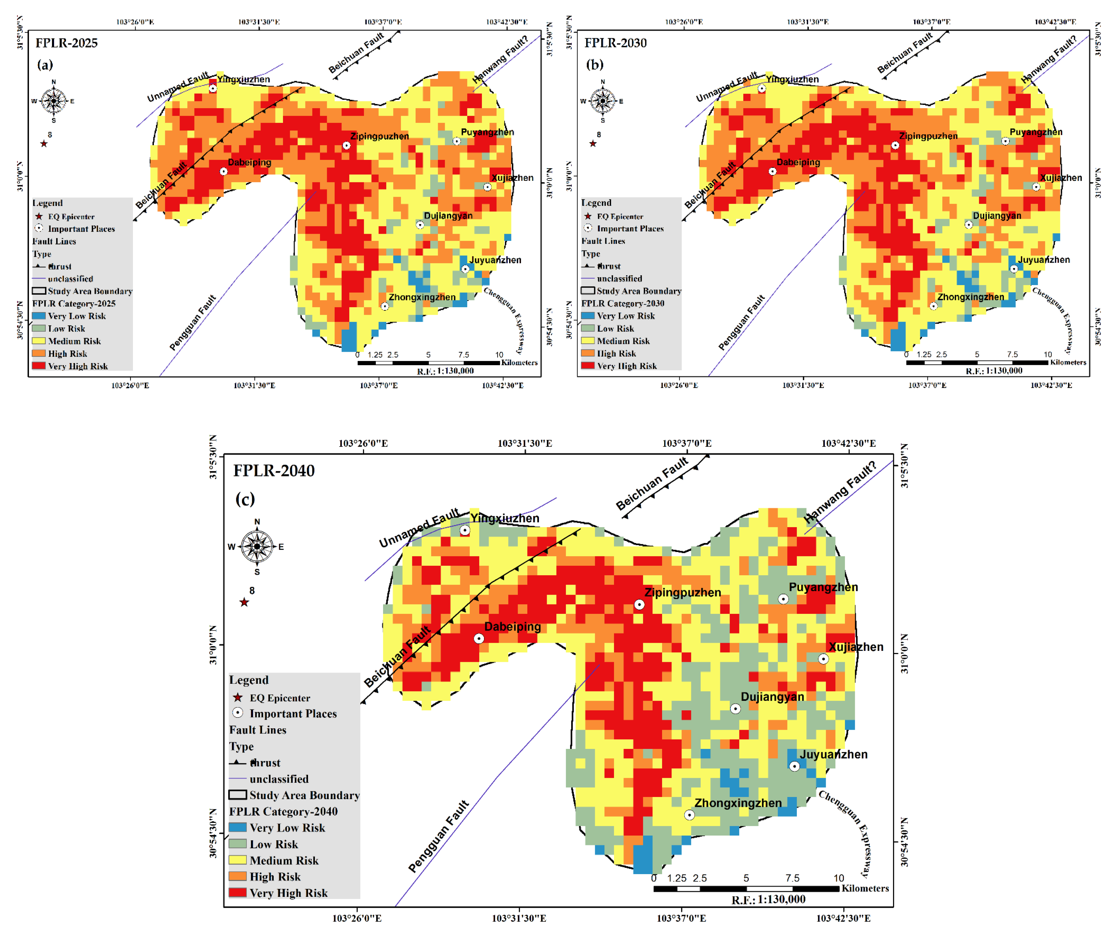
3.4. FPLR Area Identification, Mapping and Pattern of Change Analysis
4. Discussion
5. Conclusions
Supplementary Materials
Author Contributions
Funding
Acknowledgments
Conflicts of Interest
References
- Ellis, E. Land-Use and Land-Cover Change. In Encyclopedia of Earth; Cutler, J., Ed.; Environmental Information Coalition, National Council for Science and the Environment: Washington, DC, USA, 2010. [Google Scholar]
- Collins English Dictionary. Definition of Transition. Available online: https://www.collinsdictionary.com/dictionary/english/transition (accessed on 18 November 2018).
- Tendaupenyu, P.; Magadza, C.H.D.; Murwira, A. Changes in landuse/landcover patterns and humanpopulation growth in the Lake Chivero catchment, Zimbabwe. Geocarto Int. 2017, 32, 1–34. [Google Scholar] [CrossRef]
- Li, H.; Xiao, P.; Feng, X.; Yang, Y.; Wang, L.; Zhang, W.; Wang, X.; Feng, W.; Chang, X. Using Land Long-term Data Records to Map Land Cover Changes in China Over 1981–2010. IEEE J. Select. Topics Appl. Earth Observ. Remote Sens. 2017, 10, 1372–1389. [Google Scholar] [CrossRef]
- Martínez, S.; Mollicone, D. From Land Cover to Land Use: A Methodology to Assess Land Use from Remote Sensing Data. Remote Sens. 2012, 4, 1024. [Google Scholar] [CrossRef] [Green Version]
- Tiwari, M.K.; Saxena, A. Change detection of land use/landcover pattern in an around Mandideep and Obedullaganj area, using remote sensing and GIS. Int. J. Technol. Eng. Syst. 2011, 2, 398–402. [Google Scholar]
- Liu, J.Y.; Kuang, W.H.; Zhang, Z.X.; Xu, X.L.; Qin, Y.W.; Ning, J.; Zhou, W.C.; Zhang, S.W.; Li, R.D.; Yan, C.Z.; et al. Spatiotemporal characteristics, patterns and causes of land use changes in China since the late 1980s. J. Geogr. Sci. 2014, 69, 3–14. [Google Scholar] [CrossRef]
- Liu, J.; Zhang, Z.; Xu, X.; Kuang, W.; Zhou, W.; Zhang, S.; Li, R.; Yan, C.; Yu, D.; Wu, S.; et al. Spatial patterns and driving forces of land use change in China during the early 21st century. J. Geogr. Sci. 2010, 20, 483–494. [Google Scholar] [CrossRef]
- Liu, J.Y.; Liu, M.L.; Zhuang, D.F.; Zhang, Z.X.; Deng, X.Z. Study on spatial pattern of land-use change in China during 1995–2000. Sci. China Earth Sci. 2003, 46, 373–384. [Google Scholar]
- Lambin, E. The causes of land-use and land-cover change moving beyond the myths. Glob. Env. Chang. 2001, 11, 261–269. [Google Scholar] [CrossRef]
- Lambin, E.F.; Geist, H.J.; Lepers, E. Dynamics of land-use and land-cover change in tropical regions. Ann. Rev. Env. Resour. 2003, 28, 205–241. [Google Scholar] [CrossRef] [Green Version]
- Lambin, E.F.; Geist, H.J. Land-Use and Land-Cover Change: Local Processes and Global Impacts; Springer: Berlin/Heidelberg, Germany, 2006. [Google Scholar]
- Zhang, M. Progress of land science centered on land use / land cover change. Adv. Geogr. 2001, 20, 297–304. [Google Scholar]
- Zhang, Y.L.; Li, X.B.; Fu, X.F.; Xie, G.D.; Zheng, D. Urban land use change in Lhasa. Acta Geogr. Sin. 2000, 55, 395–406. [Google Scholar]
- Tahir, M.; Imam, E.; Tahir, H. Evaluation of land use/land cover changes in Mekelle City, Ethiopia using Remote Sensing and GIS. Comput. Ecol. Softw. 2013, 3, 9–16. [Google Scholar]
- Nath, B.; Niu, Z.; Singh, R.P. Land Use and Land Cover Changes, and Environment and Risk Evaluation of Dujiangyan City (SW China) Using Remote Sensing and GIS Techniques. Sustainability 2018, 10, 4631. [Google Scholar] [CrossRef] [Green Version]
- Li, F.; Liu, G. Characterizing Spatiotemporal Pattern of Land Use Change and Its Driving Force Based on GIS and Landscape Analysis Techniques in Tianjin during 2000–2015. Sustainability 2017, 9, 894. [Google Scholar] [CrossRef] [Green Version]
- Ying, C.; Ling, H.; Kai, H. Change and Optimization of Landscape patterns in a Basin Based on Remote Sensing Images: A Case Study in China. Pol. J. Env. Stud. 2017, 26, 2343–2353. [Google Scholar] [CrossRef]
- Jaafari, S.; Sakieh, Y.; Shabani, A.A.; Danehkar, A.; Nazarisamani, A. Landscape change assessment of reservation areas using remote sensing and landscape metrics (case study: Jajroud reservation, Iran). Environ. Dev. Sustain. 2015, 17, 1–17. [Google Scholar] [CrossRef]
- Seto, K.C.; Fragkias, M. Quantifying spatiotemporal patterns of urban land-use change in four cities of China with time series landscape metrics. Landsc. Ecol. 2005, 20, 871–888. [Google Scholar] [CrossRef]
- Fichera, C.R.; Modica, G.; Pollino, M. Land Cover classification and change-detection analysis using multi-temporal remote sensed imagery and landscape metrics. Eur. J. Remote Sen. 2012, 45, 1–18. [Google Scholar]
- Herold, M.; Scepan, J.; Clarke, K.C. The Use of Remote Sensing and Landscape Metrics to Describe Structures and Changes in Urban Land Uses. Environ. Plan. 2002, 34, 1443–1458. [Google Scholar] [CrossRef] [Green Version]
- Nurwanda, A.; Zain, A.F.M.; Rustiadi, E. Analysis of land cover changes and landscape fragmentation in Batanghari Regency, Jambi Province. In Proceedings of the Social and Behavioral Sciences, CITIES 2015 International Conference, Intelligent Planning Towards Smart Cities, CITIES 2015, Surabaya, Indonesia, 3–4 November 2015. [Google Scholar]
- Nagendra, H.; Munroe, D.K.; Southworth, J. From pattern to process: Landscape fragmentation and the analysis of land use/land cover change. Agric. Ecosyst. Environ. 2004, 101, 111–115. [Google Scholar] [CrossRef]
- Li, R.; Dong, M.; Cui, J.; Zhang, L.; Cui, Q.; He, W. Quantification of the impact of land-use changes on ecosystem services: A case study in Pingbian County. China. Environ. Monit. Assess. 2007, 128, 503–510. [Google Scholar] [CrossRef] [PubMed]
- Schirpke, U.; Kohler, M.; Leitinger, G.; Fontana, V.; Tasser, E.; Tappeiner, U. Future impacts of changing land-use and climate on ecosystem services of mountain grassland and their resilience. Ecosyst. Serv. 2017, 26, 79–94. [Google Scholar] [CrossRef] [PubMed]
- Tasser, E.; Leitinger, G.; Tappeiner, U. Climate change versus land-use change—What affects the mountain landscapes more? Land Use Policy 2017, 60, 60–72. [Google Scholar] [CrossRef]
- Nath, B.; Acharjee, S. Urban Municipal Growth and Landuse Change Monitoring Using High Resolution Satellite Imageries and Secondary Data: A Geospatial Study on Kolkata Municipal Corporation, Kolkata, India. Stud. Surv. Mapp. Sci. 2013, 3, 43–54. [Google Scholar]
- Bhagawat, R. Urban Growth and Land Use/Land Cover Change of Pokhara Sub-metropolitan city, Nepal. J. Theor. Appl. Inform. Technol. 2011, 26, 118–129. [Google Scholar]
- Dewan, A.M.; Yamaguchi, Y. Land use and land cover change in Greater Dhaka, Bangladesh: Using remote sensing to promote sustainable urbanization. Appl. Geogr. 2009, 29, 390–401. [Google Scholar] [CrossRef]
- Sui, L.Y.; Ming, C.B. The study framework of land use/cover change based on sustainable development in China. Geogr. Res. 2002, 21, 324–330. [Google Scholar]
- Tali, J.A.; Divya, S.; Murthy, K. Influence of urbanization on the land use change: A case study of Srinagar City. Am. J. Res. Comm. 2013, 1, 271–283. [Google Scholar]
- Rawat, J.S.; Kumar, M. Monitoring Land Use/Cover Change Using Remote Sensing and GIS Techniques: A Case Study of Hawalbagh Block, District Almora, Uttarakhand, India. Egypt. J. Remote Sens. Space Sci. 2015, 18, 77–84. [Google Scholar] [CrossRef] [Green Version]
- Appiah, D.O.; Schroeder, D.; Forkuo, E.K.; Bugri, J.T. Application of Geo-Information Techniques in Land Use and Land Cover Change Analysis in a Peri-Urban District of Ghana. Inter. J. Geo Inform. 2015, 4, 1265–1289. [Google Scholar] [CrossRef] [Green Version]
- Yu, D.; Srinivasan, S. Urban land use change and regional access: A case study in Beijing, China. Habitat Int. 2016, 51, 103–113. [Google Scholar]
- Mundia, C.N.; Aniya, M. Dynamics of land use/cover changes and degradation of Nairobi City, Kenya. Land Degrad. Dev. 2010, 17, 97–108. [Google Scholar] [CrossRef]
- Li, Y.; Zhang, Q. Human-environment interactions in China: Evidence of land-use change in Beijing-Tianjin-Hebei Metropolitan Region. Hum. Ecol. Rev. 2013, 20, 26–35. [Google Scholar]
- Dewan, A.M.; Yamaguchi, Y. Using remote sensing and GIS to detect and monitor land use and land cover change in Dhaka Metropolitan of Bangladesh during 1960–2005. Environ. Monit. Assess. 2009, 150, 237–249. [Google Scholar] [CrossRef] [PubMed]
- Lo, C.P.; Yang, X. Drivers of Land-Use/Land-Cover Changes and Dynamic Modeling for the Atlanta, Georgia Metropolitan Area. Photogramm. Eng. Remote Sens. 2002, 68, 1073–1082. [Google Scholar]
- Butt, A.; Shabbir, R.; Ahmad, S.S.; Aziz, N. Land use change mapping and analysis using Remote Sensing and GIS: A case study of Simly watershed, Islamabad, Pakistan. Egypt. J. Remote Sens. Space Sci. 2015, 18, 251–259. [Google Scholar] [CrossRef] [Green Version]
- Malik, M.I.; Bhat, M.S. Integrated Approach for Prioritizing Watersheds for Management: A Study of Lidder Catchment of Kashmir Himalayas. Environ. Manag. 2015, 54, 1267–1287. [Google Scholar] [CrossRef]
- Kaliraj, S.; Chandrasekar, N.; Ramachandran, K.K.; Srinivas, Y.; Saravanan, S. Coastal land use and land cover change and transformations of Kanyakumari coast, India using remote and GIS. Egypt. J. Remote Sens. Space Sci. 2017, 20, 169–185. [Google Scholar]
- Islam, K.; Jashimuddin, M.; Nath, B.; Nath, T.K. Land use classification and change detection by using multi-temporal remotely sensed imagery: The case of Chunati wildlife sanctuary, Bangladesh. Egypt. J. Remote Sens. Space Sci. 2018, 21, 37–47. [Google Scholar] [CrossRef]
- Islam, K.; Rahman, M.F.; Jashimuddin, M. Modeling land use change using Cellular Automata and Artificial Neural Network: The case of Chunati Wildlife Sanctuary, Bangladesh. Ecol. Indic. 2018, 88, 439–453. [Google Scholar] [CrossRef]
- Singh, R.P.; Sahoo, A.K.; Bhoi, S.; Kumar, M.G.; Bhuiyan, C.S. Ground deformation of Gujarat earthquake of 26 January 2001. J. Geol. Soc. India 2001, 58, 209–214. [Google Scholar]
- Singh, R.P.; Bhoi, S.; Sahoo, A.K.; Raj, U.; Ravindran, S. Surface manifestations after the Gujarat earthquake. Curr. Sci. 2001b, 81, 164–166. [Google Scholar]
- Singh, R.P.; Bhoi, S.; Sahoo, A.K. Significant changes in the ocean parameters after the Gujarat earthquake. Curr. Sci. 2001, 80, 1376–1377. [Google Scholar]
- Singh, R.; Simon, B.; Joshi, P.C. Estimation of surface latent heat fluxes from IRSP4/ MSMR satellite data. Proc. Indian Acad. Sci. 2001, 110, 231–238. [Google Scholar]
- Singh, R.P.; Bhoi, S.; Sahoo, A.K. Changes observed on land and ocean after Gujarat earthquake 26 January 2001 using IRS data. Int. J. Remote Sens. 2002, 23, 3123–3128. [Google Scholar] [CrossRef]
- Dey, S.; Singh, R.P. Surface Latent Heat Flux as an earthquake precursor. Nat. Hazards Earth Syst. Sci. 2003, 3, 749–755. [Google Scholar] [CrossRef]
- Okada, Y.; Mukai, S.; Singh, R.P. Changes in atmospheric aerosol parameters after Gujarat earthquake of January 26 2001. Adv. Space Res. 2004, 33, 254–258. [Google Scholar] [CrossRef]
- Dey, S.; Sarkar, S.; Singh, R.P. Anomalous changes in column water vapor after Gujarat earthquake. Adv. Space Res. 2004, 33, 274–278. [Google Scholar] [CrossRef]
- Singh, V.P.; Singh, R.P. Changes in stress pattern around epicentral region of Bhuj earthquake of 26 January 2001. Geophys. Res. Lett. 2005, 32, 1–4. [Google Scholar] [CrossRef]
- Balz, T.; Liao, M. Building-damage detection using post-seismic high-resolution SAR satellite data. Int. J. Remote Sens. 2010, 31, 3369–3391. [Google Scholar] [CrossRef]
- Guo, H.; Ma, J.; Zhang, B.; Li, Z.; Huang, J.; Zhu, L. Damage consequence chain mapping after the Wenchuan Earthquake using remotely sensed data. Int. J. Remote Sens. 2010, 31, 3427–3433. [Google Scholar] [CrossRef]
- Sowter, A. Orthorectification and interpretation of differential InSAR data over mountainous areas: A case study of the May 2008 Wenchuan Earthquake. Int. J. Remote Sens. 2010, 31, 3435–3448. [Google Scholar] [CrossRef]
- Zhuang, J.Q.; Cui, P.; Ge, Y.G.; He, Y.P.; Liu, Y.H.; Guo, X.J. Probability assessment of river blocking by debris flow associated with the Wenchuan Earthquake. Int. J. Remote Sens. 2010, 31, 3465–3478. [Google Scholar] [CrossRef]
- Pan, G.; Tang, D. Damage information derived from multi-sensor data of the Wenchuan Earthquake of May 2008. Int. J. Remote Sens. 2010, 31, 3509–3519. [Google Scholar] [CrossRef]
- Zhuang, W.; Lin, J.; Peng, J.; Lu, Q. Estimating Wenchuan Earthquake induced landslides based on remote sensing. Int. J. Remote Sens. 2010, 31, 3495–3508. [Google Scholar] [CrossRef]
- Wu, F.; Yu, B.; Yan, M.; Wang, Z. Eco-environmental research on the Wenchuan Earthquake area using Disaster Monitoring Constellation (DMC) Beijing-1 small satellite images. Int. J. Remote Sens. 2010, 31, 3643–3660. [Google Scholar] [CrossRef]
- Singh, R.P. Satellite observations of the Wenchuan Earthquake, 12 May 2008. Int. J. Remote Sens. 2010, 31, 3335–3339. [Google Scholar] [CrossRef]
- Pôças, I.; Cunha, M.; Pereira, L.S. Remote sensing-based indicators of changes in a mountain rural landscape of Northeast Portugal. Appl. Geogr. 2011, 31, 871–880. [Google Scholar] [CrossRef]
- Yi, Y.; Zhao, Y.Z.; Ding, G.D.; Cao, Y. Effects of urbanization on landscape patterns in a mountainous area: A Case Study in the Mentougou District, Beijing, China. Sustainability 2016, 8, 1190. [Google Scholar] [CrossRef] [Green Version]
- Jain, S.; Laphawan, S.; Singh, P.K. Tracing the Changes in the Pattern of Urban Landscape of Dehradun over Last Two Decades using RS and GIS. Int. J. Adv. Remote Sens. GIS 2013, 2, 351–362. [Google Scholar]
- Mottet, A.; Ladet, S.; Coque, N.; Gibon, A. Agricultural land-use change and its drivers in mountain landscapes: A case study in the Pyrenees. Agric. Ecosyst. Environ. 2006, 114, 296–310. [Google Scholar] [CrossRef]
- Wang, Z.; Lu, C.; Yang, X. Exponentially sampling scale parameters for the efficient segmentation of remote-sensing images. Int. J. Remote Sens. 2018, 39, 1628–1654. [Google Scholar] [CrossRef]
- Wang, Z.; Yang, X.; Lu, C.; Yang, F. A scale self-adapting segmentation approach and knowledge transfer for automatically updating land use/cover change databases using high spatial resolution images. Int. J. Appl. Earth Obs. Geoinf. 2018, 69, 88–98. [Google Scholar] [CrossRef]
- Arellano-Baeza, A.A.; Zverev, A.; Malinnikov, V. Study of Changes in the lineament structure, caused by earthquakes in South America by applying the lineament analysis to the ASTER (Terra) satellite data. Adv. Space Res. 2004, 33, 274–278. [Google Scholar] [CrossRef]
- Singh, S.K.; Mustak, S.; Srivastava, P.K.; Szabó, S.; Islam, T. Predicting Spatial and Decadal LULC Changes Through Cellular Automata Markov Chain Models Using Earth Observation Datasets and Geo-Information. Environ. Process. 2015, 2, 61–78. [Google Scholar] [CrossRef] [Green Version]
- Chen, L.; Nuo, W. Dynamic simulation of land use changes in Port city: A case study of Dalian, China. Procedia Soc. Behav. Sci. 2013, 96, 981–992. [Google Scholar] [CrossRef] [Green Version]
- Katana, S.J.S.; Ucakuwun, E.K.; Munyao, T.M. Detection and Prediction of Land-Cover Changes in Upper Athi River Catchment, Kenya: A Strategy Towards Monitoring Environmental Changes. Greener J. Environ. Manag. Pub. Safe. 2013, 2, 146–157. [Google Scholar] [CrossRef]
- Berger, T. Agent-Based Spatial Models Applied to Agriculture: A Simiulation Tool for Technology Diffusion, Resource Use Changes and Policy Analysis. Agri. Econom. 2001, 25, 245–260. [Google Scholar] [CrossRef]
- López, E.; Bocco, G.; Mendoza, M.; Duhau, E. Predicting Land-Cover and Land-Use Change in the Urban Fringe: A Case in Morelia City, Mexico. Landsc. Urban Plan. 2001, 55, 271–285. [Google Scholar] [CrossRef]
- Ghosh, P.; Mukhopadhyay, A.; Chanda, A.; Mondal, P.; Akhand, A.; Mukherjee, S.; Nayak, S.K.; Ghosh, S.; Mitra, D.; Ghosh, T.; et al. Application of Cellular automata and Markov-chain model in geospatial environmental modeling—A review. Remote Sens. Appl. Soc. Environ. 2017, 5, 64–77. [Google Scholar] [CrossRef]
- Baysal, G. Urban Land Use and Land Cover Change Analysis and Modeling a Case Study Area Malatya, Turkey. Master’s Thesis, Institute for Geoinformatics (IFGI), Westfälische Wilhelms-Universität, Münster, Germany, 2013. [Google Scholar]
- Mandal, U.K. Geo-information Based Spatio-temporal Modeling of Urban Land Use and Land Cover Change in Butwal Municipality, Nepal. Int. Arch. Photogramm. Remote Sens. Spat. Inf. Sci. 2014, 40, 809. [Google Scholar]
- Batty, M.; Xie, Y.; Sun, Z. Modeling urban dynamics through GIS-based cellular automata. Comput. Environ. Urban Syst. 1999, 23, 205–233. [Google Scholar] [CrossRef] [Green Version]
- Wang, Y.; Zhang, X. A Dynamic Modeling Approach to Simulating Socioeconomic Effects on Landscape Changes. Ecol. Modell. 2001, 140, 141–162. [Google Scholar] [CrossRef]
- Weng, Q. Land Use Change Analysis in the Zhujiang Delta of China Using Satellite Remote Sensing, GIS and Stochastic Modelling. J. Environ. Manag. 2002, 64, 273–284. [Google Scholar] [CrossRef] [PubMed] [Green Version]
- Aitkenhead, M.J.; Aalders, I.H. Predicting land cover using GIS, Bayesian and evolutionary algorithm methods. J. Environ. Manag. 2009, 90, 236–250. [Google Scholar] [CrossRef] [PubMed]
- Aitkenhead, M.J.; Aalders, I.H. Automating land cover mapping of Scotland using expert system and knowledge integration methods. Remote Sens. Environ. 2011, 115, 1285–1295. [Google Scholar] [CrossRef]
- Eastman, J.R. TerrSet manual. Access. TerrSet Vers. 2015, 18, 1–390. [Google Scholar]
- Houet, T.; Hubert-Moy, L. Modeling and Projecting Land-Use and Land-Cover Changes with Cellular Automaton in Considering Landscape Trajectories: An Improvement for Simulation of Plausible Future States. EARSeL eProceed, European Association of Remote Sensing Laboratories. Available online: https://halshs.archives-ouvertes.fr/halshs-00195847/document (accessed on 22 February 2020).
- Ge, Y.; Xu, J.; Liu, Q.; Yao, Y.; Wang, R. Image interpretation and statistical analysis of vegetation damage caused by the Wenchuan earthquake and related secondary disasters. J. Appl. Remote Sens. 2009, 3, 031660. [Google Scholar] [CrossRef]
- Guo, H. Guest Editorial: Remote Sensing of the Wenchuan Earthquake. J. Appl. Remote Sens. 2009, 3, 031699. [Google Scholar] [CrossRef] [Green Version]
- Han, Y.; Liu, H.; Cui, P.; Su, F.; Du, D. Hazard assessment on secondary mountain-hazards triggered by the Wenchuan earthquake. J. Appl. Remote Sens. 2009, 3, 031645. [Google Scholar]
- Jin, Y.-Q.; Wang, D. Automatic Detection of Terrain Surface Changes After Wenchuan Earthquake, May 2008, From ALOS SAR Images Using 2EM-MRF Method. IEEE Geosci. Remote Sens. 2009, 6, 344–348. [Google Scholar]
- Bardhan, R.; Debnath, R.; Bandopadhyay, S. A conceptual model for identifying the risk susceptibility of urban green spaces using geo-spatial techniques. Model. Earth Syst. Environ. 2016, 2, 1–12. [Google Scholar] [CrossRef] [Green Version]
- Ingram, K.; Knapp, E.; Robinson, J.W. Change Detection Technique Development for Improved Urbanized Area Delineation; Technical Memorandum CSC/TM-81/6087; Computer Science Corporation: Silver Springs, FL, USA; Maryland, MD, USA, 1981. [Google Scholar]
- Teixeira, Z.; Teixeira, H.; Marques, J.C. Systematic processes of land use/land cover change to identify relevant driving forces: Implications on water quality. Sci. Total Environ. 2014, 470–471, 1320–1335. [Google Scholar] [CrossRef] [PubMed] [Green Version]
- Jensen, J.R. Remote Sensing of the Environment: An Earth Resource Perspective 2/e; Pearson Education India: Noida, India, 2009. [Google Scholar]
- Richards, J.; Jia, X. Remote Sensing Digital Image Analysis; Springer: Berlin/Heidelberg, Germany, 1999. [Google Scholar]
- United Nations (UN). Transforming our world: The 2030 Agenda for sustainable development. Resolution adopted by the General Assembly on 25 September 2015. Available online: http://www.un.org/ga/search/view_doc.asp?Symbol=A/RES/70/1&Lang=E (accessed on 17 November 2018).
- USGS Earth Explorer Landsat Archive (2007–2018). Available online: https://earthexplorer.usgs.gov (accessed on 10 February 2018).
- Anderson, J.R.; Hardy, E.E.; Roach, J.T.; Witmer, R.E. A Land Use and Land Cover Classification for Use with Remote Sensor Data (USGS Professional Paper 964); Government Printing Office: Washington, DC, USA, 1976. [Google Scholar]
- Singh, A.; Singh, S.; Garga, P.K.; Khanduri, K. Land Use and Land Cover Change Detection: A Comparative Approach using Post Classification Change Matrix Function Change Detection Methodology of Allahabad City. Int. J. Curr. Eng. Technol. 2013, 3, 142–148. [Google Scholar]
- Tudes, S.; Yigiter, N.D. Preparation of land use planning model using GIS based on AHP: Case study Adana-Turkey. Bull. Eng. Geol. Environ. 2010, 69, 235–245. [Google Scholar] [CrossRef]
- Data Catalog-Data. Shapefile: Generalized Geology of the Far East (Geo3al). Metadata Creation date: March 18 2005. Available online: https://catalog.data.gov/dataset/generalized-geology-of-the-far-east-geo3al (accessed on 15 June 2019).
- Mukherjee, S.; Shashtri, S.; Singh, C.; Srivastava, P.; Gupta, M. Effect of canal on LULC using remote sensing and GIS. J. Indian Soc. Remote Sens. 2009, 37, 527–537. [Google Scholar] [CrossRef]


| SL. No. | Satellite Sensors | Year | Image Acquisition Time | Path/Row | Resolution (m) | Image Type |
|---|---|---|---|---|---|---|
| 1 | Landsat 5 TM | 2007 | 18 September 2007 | 130/38 | 30 | Level-1 GeoTIFF |
| 2 | Landsat 8 OLI | 2018 | 19 January 2018 | 130/38 | 30 | Level-1 GeoTIFF |
| 2018 | |||||||
|---|---|---|---|---|---|---|---|
| FLULC Classes | BU | F | AG | RA | WB | BL | |
| BU | 0.8987 | 0.0025 | 0.0000 | 0.0330 | 0.0148 | 0.0510 | |
| F | 0.0000 | 0.9894 | 0.0000 | 0.0098 | 0.0003 | 0.0006 | |
| 2007 | AG | 0.2292 | 0.0683 | 0.0000 | 0.1011 | 0.0000 | 0.6014 |
| RA | 0.4744 | 0.0000 | 0.0000 | 0.2385 | 0.0000 | 0.2871 | |
| WB | 0.0000 | 0.0000 | 0.0000 | 0.0303 | 0.9697 | 0.0000 | |
| BL | 0.0000 | 0.0228 | 0.5693 | 0.0000 | 0.0000 | 0.4079 | |
| Chi-Square Test | |||
|---|---|---|---|
| LULC Classes | Simulated Land Use in 2018 (O) | Actual Land Use in 2018 (E) | (O − E)2/E |
| BU | 14.94 | 18.49 | 0.68 |
| F | 38.63 | 43.73 | 0.60 |
| AG | 15.56 | 9.61 | 3.69 |
| RA | 0.89 | 5.17 | 3.55 |
| WB | 5.75 | 5.42 | 0.02 |
| BL | 24.23 | 17.58 | 2.52 |
| Total | 100.00 | 100.00 | 11.05 |
| Agreement/Disagreement | Value | Value (%) |
|---|---|---|
| Agreement Chance | 0.1429 | 14.29 |
| Agreement Quantity | 0.0961 | 9.61 |
| Agreement Strata | 0.0000 | 0.00 |
| Agreement Gridcell | 0.5127 | 51.27 |
| Disagreement Gridcell | 0.1665 | 16.65 |
| Disagreement Strata | 0.0000 | 0.00 |
| Disagreement Quantity | 0.0818 | 8.18 |
| Index | Value |
|---|---|
| Kno | 0.71 |
| Klocation | 0.76 |
| KlocationStrata | 0.76 |
| Kstandard | 0.67 |
| Total Projected Area Coverage (km2) | DD (%) between Different Times | |||||||
|---|---|---|---|---|---|---|---|---|
| LULC Classes | 2018 | 2025 | 2030 | 2040 | 2018–2025 | 2025–2030 | 2030–2040 | 2018–2040 |
| BU | 58.83 | 51.06 | 49.56 | 48.99 | −1.11 | −0.59 | −0.11 | −0.76 |
| F | 139.20 | 122.97 | 122.98 | 122.99 | −1.67 | 0.01 | 0.01 | −0.53 |
| AG | 30.58 | 42.30 | 45.00 | 46.08 | 5.47 | 1.28 | 0.24 | 2.30 |
| RA | 16.47 | 1.84 | 2.28 | 2.40 | −12.69 | 4.78 | 0.53 | −3.88 |
| WB | 55.96 | 81.28 | 19.76 | 79.16 | 6.46 | −0.37 | −0.07 | 1.88 |
| BL | 17.26 | 18.85 | 18.72 | 18.68 | 1.32 | −0.14 | −0.02 | 0.37 |
| Total | 318.30 | 318.30 | 318.30 | 318.30 | ||||
| LULC Classes | Total Projected Area Coverage (%) | Projected Gain/Loss (%) between Different Times | |||||||
|---|---|---|---|---|---|---|---|---|---|
| 2018 | 2025 | 2030 | 2040 | 2018–2025 | 2025–2030 | 2030–2040 | 2018–2040 | ||
| BU | 18.49 | 16.04 | 15.57 | 15.39 | −2.45 | −0.47 | −0.18 | −3.10 | |
| F | 43.73 | 38.63 | 38.64 | 38.64 | −5.10 | 0.01 | 0.00 | −5.09 | |
| AG | 9.61 | 13.29 | 14.14 | 14.48 | 3.68 | 0.85 | 0.34 | 4.87 | |
| RA | 5.17 | 0.58 | 0.72 | 0.75 | −4.59 | 0.14 | 0.03 | −4.42 | |
| WB | 17.58 | 25.54 | 25.06 | 24.87 | 7.96 | −0.48 | −0.19 | 7.29 | |
| BL | 5.42 | 5.92 | 5.88 | 5.87 | 0.50 | −0.04 | −0.01 | 0.45 | |
| Total | 100.00 | 100.00 | 100.00 | 100.00 | |||||
| Given: | Transition Probabilities of Changing to: | ||||||
|---|---|---|---|---|---|---|---|
| FLULC Classes | Year | BU | F | AG | RA | WB | BL |
| 2018–2025 | 0.9763 | 0.0002 | 0.0004 | 0.0009 | 0.0112 | 0.0111 | |
| BU | 2025–2030 | 0.9888 | 0.0000 | 0.0000 | 0.0000 | 0.0080 | 0.0032 |
| 2030–2040 | 0.9900 | 0.0000 | 0.0000 | 0.0000 | 0.0072 | 0.0028 | |
| 2018–2025 | 0.0000 | 0.9943 | 0.0020 | 0.0027 | 0.0003 | 0.0007 | |
| F | 2025–2030 | 0.0000 | 1.0000 | 0.0000 | 0.0000 | 0.0000 | 0.0000 |
| 2030–2040 | 0.0000 | 1.0000 | 0.0000 | 0.0000 | 0.0000 | 0.0000 | |
| AG | 2018–2025 2025–2030 | 0.0737 0.0495 | 0.0000 0.0000 | 0.8456 0.8928 | 0.0047 0.0007 | 0.0000 0.0000 | 0.0760 0.0571 |
| 2030–2040 | 0.0355 | 0.0000 | 0.9230 | 0.0005 | 0.0000 | 0.0410 | |
| 2018–2025 | 0.3489 | 0.0000 | 0.0012 | 0.6339 | 0.0000 | 0.0161 | |
| RA | 2025–2030 | 0.2549 | 0.0000 | 0.0000 | 0.7334 | 0.0000 | 0.0117 |
| 2030–2040 | 0.1443 | 0.0000 | 0.0000 | 0.8487 | 0.0000 | 0.0069 | |
| 2018–2025 | 0.0000 | 0.0000 | 0.0000 | 0.0010 | 0.9990 | 0.0001 | |
| WB | 2025–2030 | 0.0000 | 0.0000 | 0.0000 | 0.0000 | 1.0000 | 0.0000 |
| 2030–2040 | 0.0000 | 0.0000 | 0.0000 | 0.0000 | 1.0000 | 0.0000 | |
| 2018–2025 | 0.0000 | 0.0002 | 0.0033 | 0.0002 | 0.0000 | 0.9963 | |
| BL | 2025–2030 | 0.0000 | 0.0000 | 0.0000 | 0.0000 | 0.0000 | 1.0000 |
| 2030–2040 | 0.0000 | 0.0000 | 0.0000 | 0.0000 | 0.0000 | 1.0000 | |
| a. | ||||||
| Total Risk Weight Class Range | Risk Category | Risk Area (km2) | Risk Area (%) | Geological Zone under Risk | Landscape Type under Risk (Priority Based) | Important Locations under Risk |
| 13–18 | Very Low | 6.53 | 2.05 | Zone- III, IV, II | BU, AG, WB, F, BL | 4, 5 |
| 18–20 | Low | 16.25 | 5.11 | Zone- IV, III, II | BU, BL, WB | 4, 8, 6, 5, 7 |
| 20–23 | Medium | 116.21 | 36.51 | Zone- IV, III, II, I | BU, F, AG, BL | 6, 3, 4, 5, 8, 3, 2 |
| 23–25 25–31 | High Very High | 110.21 69.10 | 34.62 21.71 | Zone-I, IV, II, III Zone- II, I, IV | F, BU, AG, BL WB, AG, F, BU, BL | 1, 2, 3, 4, 7, 6, 8 2, 3, 4, 8, 7 |
| Total | 318.30 | 100.00 | ||||
| b. | ||||||
| Total Risk Weight Class Range | Risk Category | Risk Area (km2) | Risk Area (%) | Geological Zone under Risk | Landscape type under Risk (priority based) | Important Locations under Risk |
| 13–18 | Very Low | 7.28 | 2.29 | Zone- III, IV | BU, AG, WB | 4, 5 |
| 18–20 | Low | 17.78 | 5.59 | Zone- IV, III, II | AG, WB, BU, BL | 5, 6, 7, 8, 1, 3 |
| 20–23 | Medium | 112.02 | 35.19 | Zone- IV, III, II, I | BU, AG, F, BL | 4, 5, 6, 7, 8, 3, 1 |
| 23–25 25–31 | High Very High | 111.12 70.10 | 34.91 22.02 | Zone- I, II, IV, III Zone- II, I, IV | F, AG, BL, WB WB, F, AG, BU, BL | 1, 2, 3, 5, 7, 8 3, 2, 1, 8, 7, 6 |
| Total | 318.30 | 100.00 | ||||
| c. | ||||||
| Total Risk Weight Class Range | Risk Category | Risk Area (km2) | Risk Area (%) | Geological Zone under Risk | Landscape Type under Risk (Priority Based) | Important Locations under Risk |
| 13–18 | Very Low | 7.28 | 2.29 | Zone-III, IV, II | BU, AG, BL | 4, 5 |
| 18–20 | Low | 75.10 | 23.59 | Zone- IV, III, II, I | BU, F, AG, WB | 4, 5, 6, 7, 1 |
| 20–23 | Medium | 111.38 | 34.99 | Zone- IV, I, II, III | F, AG, BU, BL | 8, 1, 4, 5, 6, 7 |
| 23–25 25–31 | High Very High | 54.40 70.14 | 17.09 22.04 | Zone-I, II, IV Zone-II, I, IV | F, AG, BL WB, AG, BU, BL, F | 2, 3, 7, 8 3, 2, 1, 8, 7 |
| Total | 318.30 | 100.00 | ||||
© 2020 by the authors. Licensee MDPI, Basel, Switzerland. This article is an open access article distributed under the terms and conditions of the Creative Commons Attribution (CC BY) license (http://creativecommons.org/licenses/by/4.0/).
Share and Cite
Nath, B.; Wang, Z.; Ge, Y.; Islam, K.; P. Singh, R.; Niu, Z. Land Use and Land Cover Change Modeling and Future Potential Landscape Risk Assessment Using Markov-CA Model and Analytical Hierarchy Process. ISPRS Int. J. Geo-Inf. 2020, 9, 134. https://0-doi-org.brum.beds.ac.uk/10.3390/ijgi9020134
Nath B, Wang Z, Ge Y, Islam K, P. Singh R, Niu Z. Land Use and Land Cover Change Modeling and Future Potential Landscape Risk Assessment Using Markov-CA Model and Analytical Hierarchy Process. ISPRS International Journal of Geo-Information. 2020; 9(2):134. https://0-doi-org.brum.beds.ac.uk/10.3390/ijgi9020134
Chicago/Turabian StyleNath, Biswajit, Zhihua Wang, Yong Ge, Kamrul Islam, Ramesh P. Singh, and Zheng Niu. 2020. "Land Use and Land Cover Change Modeling and Future Potential Landscape Risk Assessment Using Markov-CA Model and Analytical Hierarchy Process" ISPRS International Journal of Geo-Information 9, no. 2: 134. https://0-doi-org.brum.beds.ac.uk/10.3390/ijgi9020134