Identification of Urban Functional Regions in Chengdu Based on Taxi Trajectory Time Series Data

Abstract

Overall scientific planning of urbanization layout is an important component of the new period of land spatial planning policies. Defining the main functions of different spaces and dividing urban functional areas are of great significance for optimizing the land development pattern. This article identifies and analyses urban functional areas from the perspective of data mining. The results of this method are consistent with the actual situation. In this paper, representative taxi trajectory data are selected as the research basis of urban functional areas. First, based on trajectory data from Didi Chuxing within the high-speed road surrounding Chengdu, we generated trajectory time sequence data and used the dynamic time warping (DTW) algorithm to generate a time series similarity matrix. Second, we utilized the K-medoid clustering algorithm to generate preliminary results of land clustering and selected the results with high classification accuracy as the training samples. Then, the k-nearest neighbour (KNN) classification algorithm based on DTW was performed to classify and identify the urban functional areas. Finally, with the help of point-of-interest (POI) auxiliary analysis, the final functional layout in Chengdu was obtained. The results show that the spatial structure of Chengdu is complex and that the urban functions are interlaced, but there are still rules that are followed. Moreover, traffic volume and inflow data can better reflect the travel rules of residents than simple taxi on–off data. The original DTW calculation method has high temporal complexity, which can be improved by normalization and the reduction of time series dimensionality. The semi-supervised learning classification method is also applicable to trajectory data, and it is best to select training samples from unsupervised learning. This method can provide a theoretical basis for urban land planning and has auxiliary and guiding value for urbanization layout in the context of land spatial planning policies in the new era.

1. Introduction

An urban functional area is a product of nature, society and the economy that enables a city to simultaneously support a variety of human activities, such as work, life, dining and entertainment [1]. Overall scientific planning for urbanization is an important part of the national spatial planning policy in the new era. Determining and dividing the main functions of different spaces is the basis for determining the direction of urban land development, which is of great significance for standardizing the process and optimizing the patterns of national land development.

The distribution of urban spatial structures and functions has consistently been an important topic in urban research. Traditional studies on urban spatial structure are based on the analysis of the interaction between urban functions and social processes [2]. With the development of remote sensing technology, the use of remote sensing images to detect land-use change has become an important means to study urban functions [3,4,5]. Many scholars have applied data with location information to the study of urban space. Ahas et al. [6] first proposed that mobile phone location data could be applied to the study of urban spatial structure. Subsequently, Ratti et al. [7], based on Ahas, demonstrated the results of analysing the spatial and temporal changes of urban activities using thermal maps to mobile phone data, opening the research field of the application of mobile positioning data to a large sample, a large range and a dynamic understanding of urban systems.

In recent years, the information age has deepened, and the analysis of urban functional areas from the perspective of location-based service (LBS) data mining has become mainstream. Various types of social media data often contain location information. Cranshaw [8] introduced a clustering model and research methodology for studying the structure and composition of a city on a large scale based on the social media its residents generate. Kling et al. [9] explored the use of textual and event-based citizen-generated data from services such as Twitter and Foursquare to study urban dynamics. Steiger [10] introduced the utilization of social media data to investigate urban environments. Dong [11] extracted population flow information from WeChat data to explain the urban space.

With the emergence of smartphones with positioning functions, the location information contained in mobile phone data represents the law of human activities. Therefore, many scholars use mobile phone data to reveal the laws related to urban functions. Phithakkitnukoon et al. [12] studied the travel patterns of mobile phone users in Japan using mobile data. Victor Soto et al. [13] designed an automatic land use identification system based on the signal generated by the cell phone base station network. Becker R.A. et al. [14] analysed the population flow in New York City and its suburbs by using cellular data (CDR).

As spatiotemporal trajectory data become increasingly easy to obtain, scholars have studied user behaviour patterns, traffic volume, regional population density, occupation and housing distribution and other issues by analysing the trajectory and then drawing conclusions related to the urban functional structure. For example, Brockman [15] used travel bugs to understand human mobility patterns. Doyle [16] used cell phone data combined with the Markov chain to analyse population density and thus to draw conclusions about the behaviour of urban residents. Yuan et al. [17] proposed a framework named DRoF (Discover Regions of different Functions) to divide Beijing into nine functional areas using this framework.

With regard to tracking data, public transportation data play an important role in expressing residents’ behavioural activities. Therefore, this type of data has become a practical tool to extract residents’ activity rules and summarize urban functions. Sun et al. [18] used smart card data to extract the space–time density of human activities and the track of trains. Zhong et al. [19] proposed a method to infer urban functions at the building level using transportation data obtained from surveys and smart card systems. Han et al. [20] used bus card swipe data to extract the rules of public transportation use by residents and then identified the functional areas of Beijing. Point-of-interest (POI) data are often used as auxiliary interpretation data for urban function analysis in scholars’ studies [21].

As the main mode of transport for citizens, taxi travel largely reflects the spatial and temporal patterns of urban population movement, so taxi trajectory data are widely applied to study urban functional areas. Liu [22] analysed the global spatial–temporal pattern of trips and explored urban land use with GPS-enabled taxi data. Pan et al. [23] used time series extracted from taxi track data to classify urban functional areas. Chen et al. [24] used GPS data of floating vehicles to identify functional areas of Guangzhou from the perspective of semantic analysis. However, previous studies on the temporal characteristics of mined data are not sufficient. In addition, the direct clustering method, namely, unsupervised learning, was used in most time series mining studies, and there may be many inaccuracies in category definitions in unsupervised learning because of the lack of accurate data labels for the training sample.

Therefore, this paper adopts a semi-supervised learning method that combines clustering and classification to perform data mining. First, K-medoid clustering is conducted based on the similarity of time series data, which is calculated by the dynamic time warping (DTW) algorithm. Accurate results are selected as training samples. Then, k-nearest neighbour (KNN) classification is performed on similar time series data based on the training samples generated in the previous step, and accurate classification results are obtained. Finally, POI analysis is used to analyse the specific functions of various functional areas. This paper provides a new way of thinking about the application of trajectory data mining in the identification of urban function. In the context of national spatial planning policies in the new era, these results have reference value for the systematic understanding of urban spatial structure and decision support for the scientific planning of urbanization layout.

2. Materials and Methods

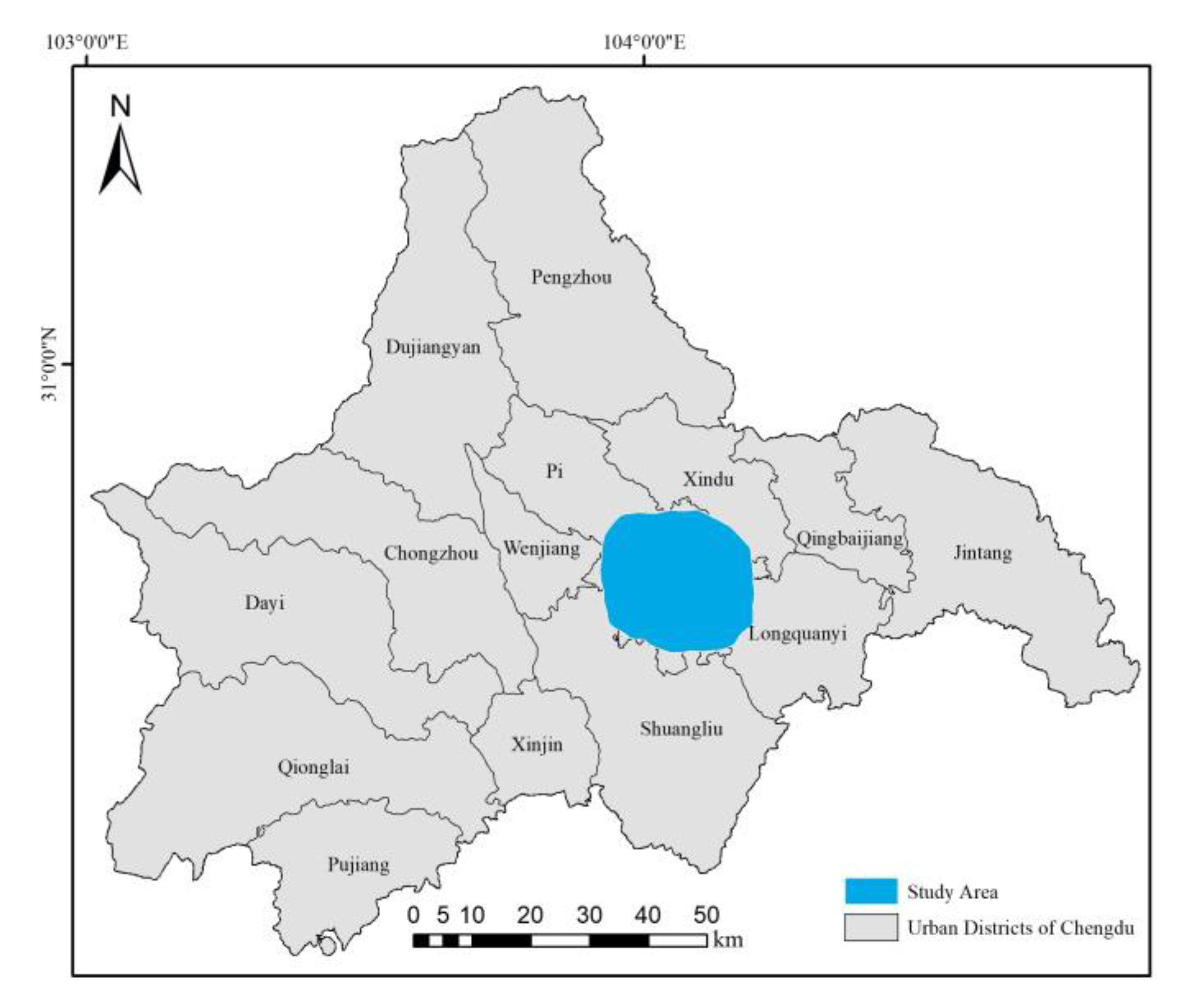
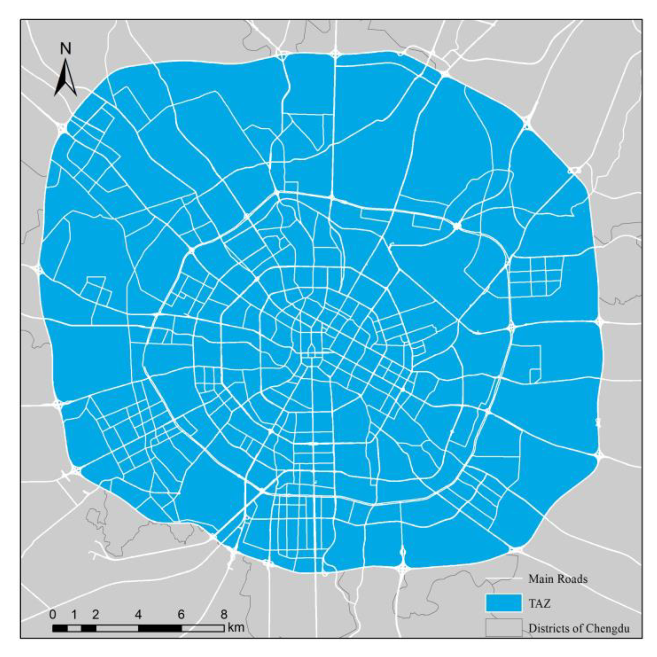
2.1. Study Area

Chengdu, the capital of Sichuan Province, is a crucial national high-tech industrial base and an important central city in the western region. According to the official website of the People′s Government of Chengdu (http://www.chengdu.gov.cn/), by 2018, Chengdu covered an area of 14,335 square kilometres and had a permanent population of 16.33 million and a GDP of 1534.277 billion yuan. The research area of this paper is within the beltway of Chengdu, including the urban land of Qingyang District, Jinniu District, Chenghua District, Jinjiang District, Wuhou District and other districts and counties. As a modern metropolis, Chengdu has a complicated urban land and spatial structure, and various urban functions are staggered, but there are still rules to follow. This paper studies the complex distribution of functions in Chengdu from the perspective of big data mining. The study area is shown in Figure 1.

2.2. Study Data and Preprocessing

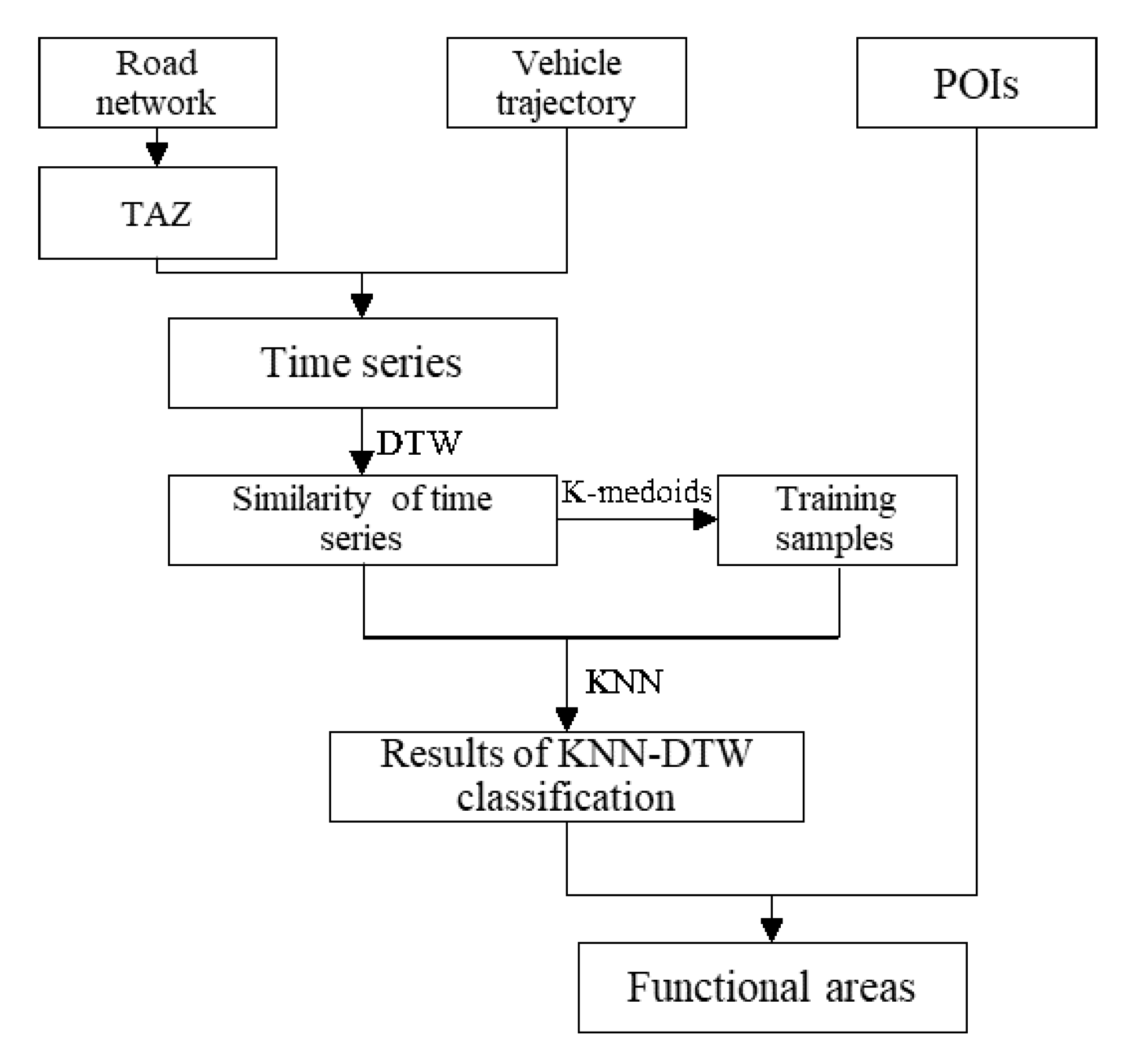
The main data used in this paper are Chengdu road network data, vehicle trajectory data and POI data. The unified coordinate system is CGCS2000_3_Degree_GK_CM_105E.

Chengdu road network data, which were collected from Gaode Map, were used to generate a traffic analysis zone (TAZ). The TAZ is a useful tool for analysing complex urban traffic networks because there are similar characteristics and strong correlations of traffic in the same TAZ [8]. Therefore, the TAZ was taken as the basic spatial unit in the analysis of urban functional structure in this paper. After removing unnecessary details (overpasses, roundabouts, etc.), the five grades of highways, urban expressways, national highways, provincial highways, and urban trunk roads were used to divide the study area into 422 TAZs (Figure 2).

Vehicle trajectory data were acquired from the GAIA open data initiative (https://gaia.didichuxing.com) of Didi Chuxing. Didi Chuxing, which is a travel platform for taxi, private car, express, driving and bus services, has changed the traditional way of taking a taxi and led the development of modern travel in the era of mobile Internet. In this study, a total of 3,298,395 records were selected from the order data for 14 days from 7 November 2016 (Monday), to 20 November 2016 (Sunday). After cleaning and preprocessing the original data, each record contained a unique identifier ID, the order start and end time and the start and endpoint locations (latitude and longitude).

POI data were acquired from the open platform of Gaode Map (https://lbs.amap.com), a leading provider of digital map content, navigation and location services in China. This study used this open platform to collect POI data in December 2016 within the beltway of Chengdu, with a total of 560,369 records. The original POI data were classified into various categories covering a variety of subcategories, and there were overlapping problems in different categories, so it was necessary to delete and reclassify the POI data. Referring to the latest version from 2011 of the "Standard of urban land classification and planning construction land of China (GB50137-2011)" and considering the type and attributes of urban functional areas, this paper divided the POI data into the following categories: catering, shopping services, leisure services, accommodation services, science and education services, healthcare services, dwellings, companies, government agencies and social organizations, and tourist attractions.

2.3. Methods

In the study of time series data, clustering is a common data mining method. However, due to the lack of accurate data labels for the training samples, there may be many inaccurate category definitions in the results of the clustering algorithm. Therefore, this paper adopts a semi-supervised learning method that combines clustering and classification to perform data mining. The core method of this paper is based on DTW calculation and the KNN classification method to classify urban functional areas. Since there were no training samples in the current situation, the training samples were first selected by combining K-medoid clustering based on DTW and analysing the baselines of the time series data. Then, KNN classification based on DTW was performed, and finally, POI analysis was used to analyse the specific functions of various functional areas. The specific research process is shown in Figure 3.

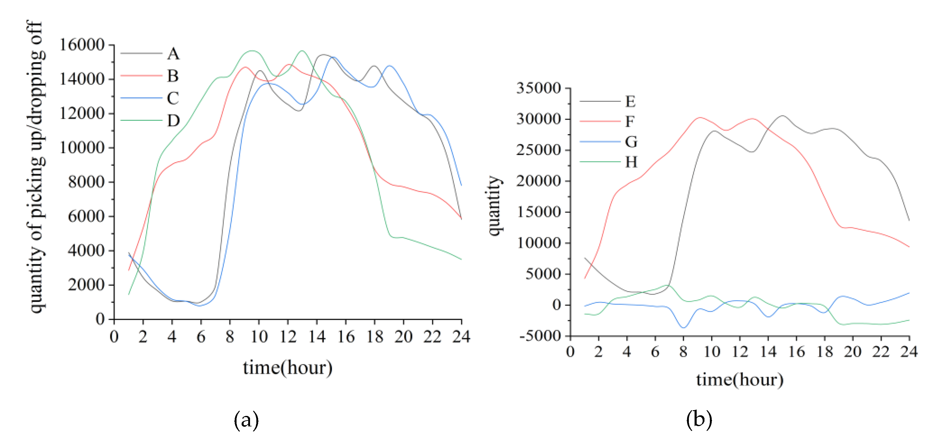
2.3.1. Methods of Time Series Generation

To understand the travel patterns of residents, the average daily and hourly pickup and drop-off times on weekdays and weekends in the study area were counted (Figure 4a). On this basis, the hourly traffic volume (pickup + drop-off) and inflow (drop-off − pickup) on weekdays and weekends were calculated and counted (Figure 4b).

Figure 4 shows that there are large differences in the travel patterns of residents on working days and rest days, so working days and rest days should be treated separately. The pickup and drop-off point data on weekdays and weekends intersect with the TAZ data. Then, the pickup and drop-off numbers within each hour and each TAZ were counted. Finally, the average passenger numbers over 24 h a day on weekdays and weekends were calculated. We obtained 4 sets of data in 422 TAZs: pickup quantity on weekdays, dropoff quantity on weekdays, pickup quantity on weekends and dropoff quantity on weekends [25].

It can be seen from Figure 4 that the independent analysis of the pickup and drop-off quantities does not adequately reflect the travel pattern. Therefore, adding traffic volume (pickup + drop-off) and inflow (drop-off − pickup) to the time series can better reflect the travel characteristics of residents. In addition, considering that this research unit is a TAZ generated by cutting roads rather than a regular grid division, the area differences between each research unit are large, so the density of each unit should be used to create the time series.

In summary, the time series of each ultimately generated research unit is 96 dimensions:

$$\left\{T_0,T_1,\dots ,T_{23},T_{24},T_{25},\dots ,T_{47},I_0,I_1,\dots ,I_{23},I_{24},I_{25},\dots ,I_{47}\right\}$$

(1)

where $T_0~T_{23}$ represents the traffic volume per unit area on working days, $T_{24}~T_{47}$ represents the traffic volume per unit area on rest days, $I_0~I_{23}$ represents the inflow per unit area on working days, and $I_{24}~I_{47}$ represents the inflow per unit area on rest days. Time series for 422 plots were generated.

2.3.2. Dynamic Time Warping

In essence, the clustering problem of time series involves how to better measure the similarity of 2 time series [26]. The methods for measuring the similarity of time series can be generally divided into three categories: time, shape and variation [27]. This paper focuses on the time series of taxi traffic volume, whose shape characteristics (rise, fall, extremum) are the response to residents’ travel patterns. In the methods of the time series similarity measurement based on the shape, the DTW algorithm applies the constraints of the structured time dimension to find the best correspondence between the 2 observed sequences and can mine similarities and differences of the time sequences with maximum flexibility. Therefore, DTW has practically become the best distance measurement method of time series similarity calculation [28].

To eliminate migration and scaling in the process of data collection, Z-normalization is first performed for the original time series. It is assumed that T is the original time series and Z is the Z-normalized time series:

$$T=\{t_1,t_2,\dots ,t_k,\dots ,t_n\}$$

(2)

$$Z=\{z_1,z_2,\dots ,z_k,\dots ,z_n\}$$

(3)

Then,

$$z_i=\frac{t_i-{\mu }_T}{{\sigma }_T}$$

(4)

where ${\mu }_T$ and ${\sigma }_T$ are the arithmetic mean value and standard variance of sequence $T$ and $Z$, respectively:

$${\mu }_T=\frac{1}{n}{{\displaystyle \sum }}_{i-1}^n{t}_i$$

(5)

$${\sigma }_T=\sqrt{\frac{1}{m-1}{{\displaystyle \sum }}_{i-1}^n\left(t_i-{\mu }_T\right)}$$

(6)

To improve the efficiency of data processing, the piecewise aggregate approximation (PAA) algorithm is adopted here to reduce the dimensionality of the data:

$$Z_{\mathrm{PAA}\left(i\right)}=\frac{1}{P}{{\displaystyle \sum }}_{j=P\left(i-1\right)+1}^{Pi}{Z}_i$$

(7)

In this algorithm, every P data point in the sequence is averaged, and the new value generated is a sampling point of the new sequence that is dimensionally reduced [29].

After dimension reduction, DTW was conducted to measure the similarity of 2 sequences. It is assumed that both A and B are time series after Z-normalization and PAA dimension reduction:

$$\mathrm{A}=\{a_1,a_2,\dots ,a_i,\dots ,a_n\}$$

(8)

$$\mathrm{B}=\{b_1,b_2,\dots ,b_j,\dots ,b_m\}$$

(9)

The DTW algorithm first establishes an n × m matrix MAR. Each element in the matrix represents the distance between point $a_i$ and point $b_i$ [30]:

$$MAR\left(i,j\right)=d\left(a_i,b_j\right)$$

(10)

$$d\left(a_i,b_j\right)={\left(a_i-b_j\right)}^2$$

(11)

DTW then finds the shortest path in the matrix MAR from the element at the bottom left to the element at the top right, satisfying 3 constraints: boundary conditions, continuity conditions, and monotone conditions. The boundary condition means that the starting point of the path is the element in the lower left corner of the matrix and the ending point is the element in the upper right corner. The continuity condition means that, except for the starting and ending points, 2 points must be adjacent around each element in the path. The monotonicity condition requires that the next element on the path must be to the right of or above the previous element and must not span 2 elements. Among all the paths that meet the above three constraints, DTW selects the shortest path:

$$d_{\mathrm{DTW}}\left(i,j\right)=MAR\left(i,j\right)+\min \left(d_{\mathrm{DTW}}\left(i,j-1\right),d_{\mathrm{DTW}}\left(i-1,j\right),d_{\mathrm{DTW}}\left(i-1,j-1\right)\right)$$

(12)

where $d_{\mathrm{DTW}}\left(i,j\right)$ refers to the minimum cumulative distance of the current elements $MAR\left(i,j\right)$ and $d_{\mathrm{DTW}}\left(0,0\right)=0,d_{\mathrm{DTW}}\left(0,j\right)=d_{\mathrm{DTW}}\left(i,0\right)=\infty$.

2.3.3. K-Medoids

For a large amount of data without labels, semi-supervised learning usually adopts manual methods to mark a small number of data labels with typical characteristics and uses them as training samples to train most of the remaining data without labels [31]. In this paper, training samples are generated by combining unsupervised learning with manual labelling. K-medoid clustering based on DTW calculation was adopted, and typical and accurate data were selected as training samples for semi-supervised classification according to the time series baseline in the clustering results.

Using the DTW algorithm, we can obtain the plot distance matrix, that is, the similarity matrix of the time series of taxi traffic volume for 422 plots. Based on this matrix, we can distinguish the differences of the different plot types [32]. In the generation of training samples, the clustering method adopted in this paper is K-medoids, which is the preferred large-scale data clustering analysis method. The difference between K-medoids and the K-means algorithm is that the centre point selection in the K-means algorithm is the focus of all points in the current cluster; however, the centre point selection in K-medoids exists in the current cluster, and the sum of the distances between all other points in the current class and this centre point is the smallest, so K-medoids are less affected by outliers [33].

The size of the data set, the purpose of classification and the validity of the clustering effect should be considered comprehensively to determine the number of clusters, K [25]. To evaluate the impact of different clustering numbers on the reliability of the clustering results, the clustering number reliability should be evaluated by the silhouette coefficient, which can be calculated by repeatedly conducting clustering operations [33]:

$$S\left(i\right)=\frac{b\left(i\right)-a\left(i\right)}{\min \left\{a\left(i\right),b\left(i\right)\right\}}$$

(13)

where $a\left(i\right)$ represents the mean value of the DTW distance between sample point $i$ and other sample points in the same cluster and $b\left(i\right)$ represents the mean value of the minimum DTW distance between sample point $i$ and other clusters. The larger the value of $S\left(i\right)$ is, the better the matching degree between the sample point $i$ and the existing clustering results. When $S\left(i\right)$ is a negative value, it indicates that the sample point $i$ should be aggregated into neighbouring clusters.

2.3.4. K-Nearest Neighbour

The k-nearest neighbour (KNN) classification algorithm is a simple but effective algorithm in data mining classification technology. The basic idea of this algorithm is that the sample to be classified belongs to the group of classified samples with k-nearest neighbours. The time series data of traffic volume belong to the data type with many overlapping class domains. Therefore, compared with the classification method that relies on class domain discrimination, KNN mainly relies on the limited neighbouring samples as the classification basis, which has better applicability.

In this paper, the KNN method based on DTW calculation was adopted to classify the time series data. DTW can help to calculate the minimum path between time series curves, which was used to replace the Euclidean distance in the KNN algorithm for time series clustering [34]. Experience shows that when combined with DTW, the nearest neighbour algorithm works best when K = 1 (i.e., 1 nearest neighbour classification) [35,36].

2.3.5. POI Auxiliary Analysis

After K-medoid clustering and KNN classification of the time series, the differences in urban land types are determined. Then, specific functional types of each category should be identified. In this paper, the definition of function was mainly determined according to the POI types in the clusters. A POI contains semantic information on urban functions and plays an important role in understanding the spatial and temporal utilization of urban space [1]. The frequency density (FD) and category ratio (CR) of POIs are usually used to determine the specific function of one region [37]:

$$F{D}_{ij}=\frac{n_i}{S_j}\left(i=1,2,\dots ,10;j=1,2,\dots ,N\right)$$

(14)

where $N$ refers to the number of plot types after clustering,$n_i$ refers to the number of the POI type $i$ in cluster $j,S_j$ refers to the total area of cluster $j$, and therefore $F{D}_{ij}$ represents the density of POI type $i$ in cluster $j$. However, from the preprocessing of POI data, it can be found that there is a large difference in the number of POIs of different categories. To eliminate the impact, min–max standardization should be carried out to $F{D}_{ij}$ [38,39]:

$$F{D}_{nor}\left(i,j\right)=\frac{F{D}_{i,j}-F{D}_{\min }}{F{D}_{\max }-F{D}_{\min }}\left(i=1,2,\dots ,10;j=1,2,\dots ,N\right)$$

(15)

Then, the normalized frequency density is used to calculate the category ratio:

$$C{R}_{i,j}=\frac{F{D}_{nor}\left(i,j\right)}{{{\displaystyle \sum }}_{i=1}^{10}F{D}_{nor}\left(i,j\right)}\times 100\%\left(i=1,2,\dots ,10;j=1,2,\dots ,N\right)$$

(16)

3. Results

3.1. Generation of the Training Sample

To obtain training samples of semi-supervised learning, the K-medoids algorithm was utilized to cluster the preprocessed time series data. First, through repeated clustering operations, the reliability of the number of clusters is evaluated by the silhouette coefficient. The change in the silhouette value with the number of clusters K is shown in Figure 5. The larger the silhouette value is, the better the clustering effect will be. The clustering results are shown in Figure 6. At this point, based on the trajectory time series data, the land is divided into six clusters (C1~C6), but the specific functions of each cluster are still unknown. However, we can see from the figure that the functional distribution of the study area is a ring structure. Then, the baseline of the time series of each cluster was taken as the evaluation standard, and data with good clustering effects of 20% were selected as the training samples. The results are shown in Figure 7.

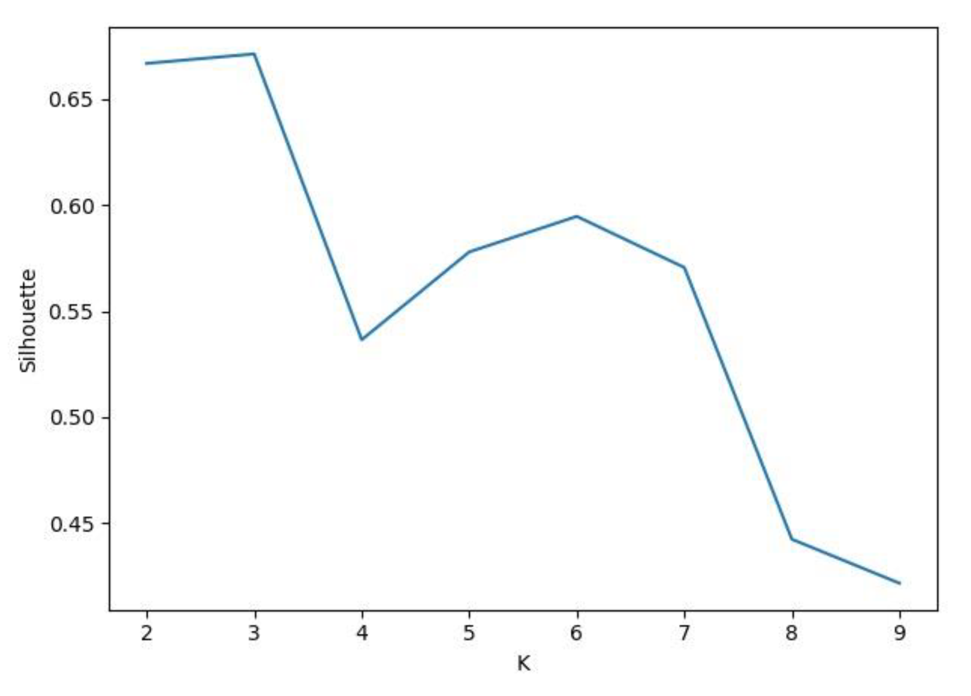
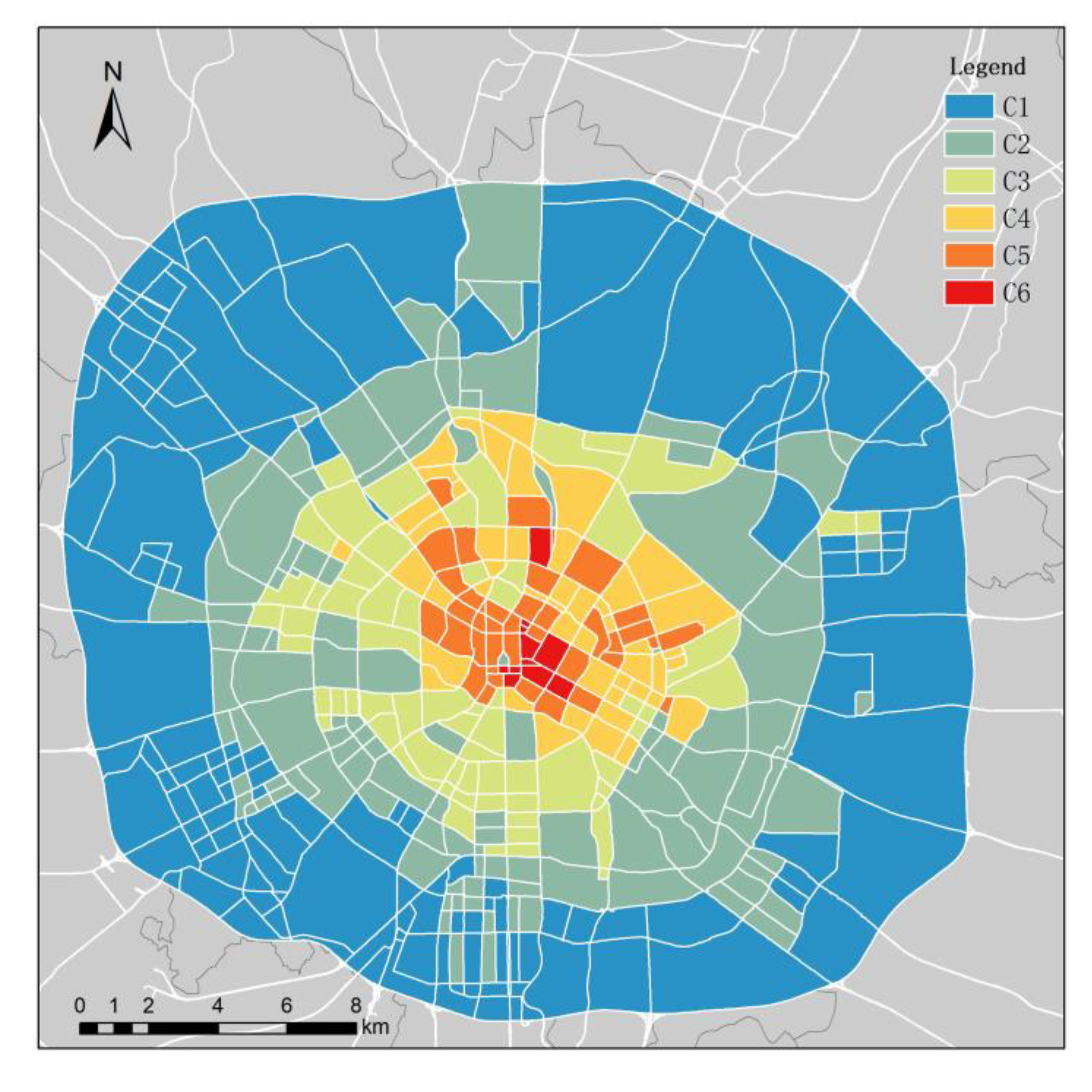
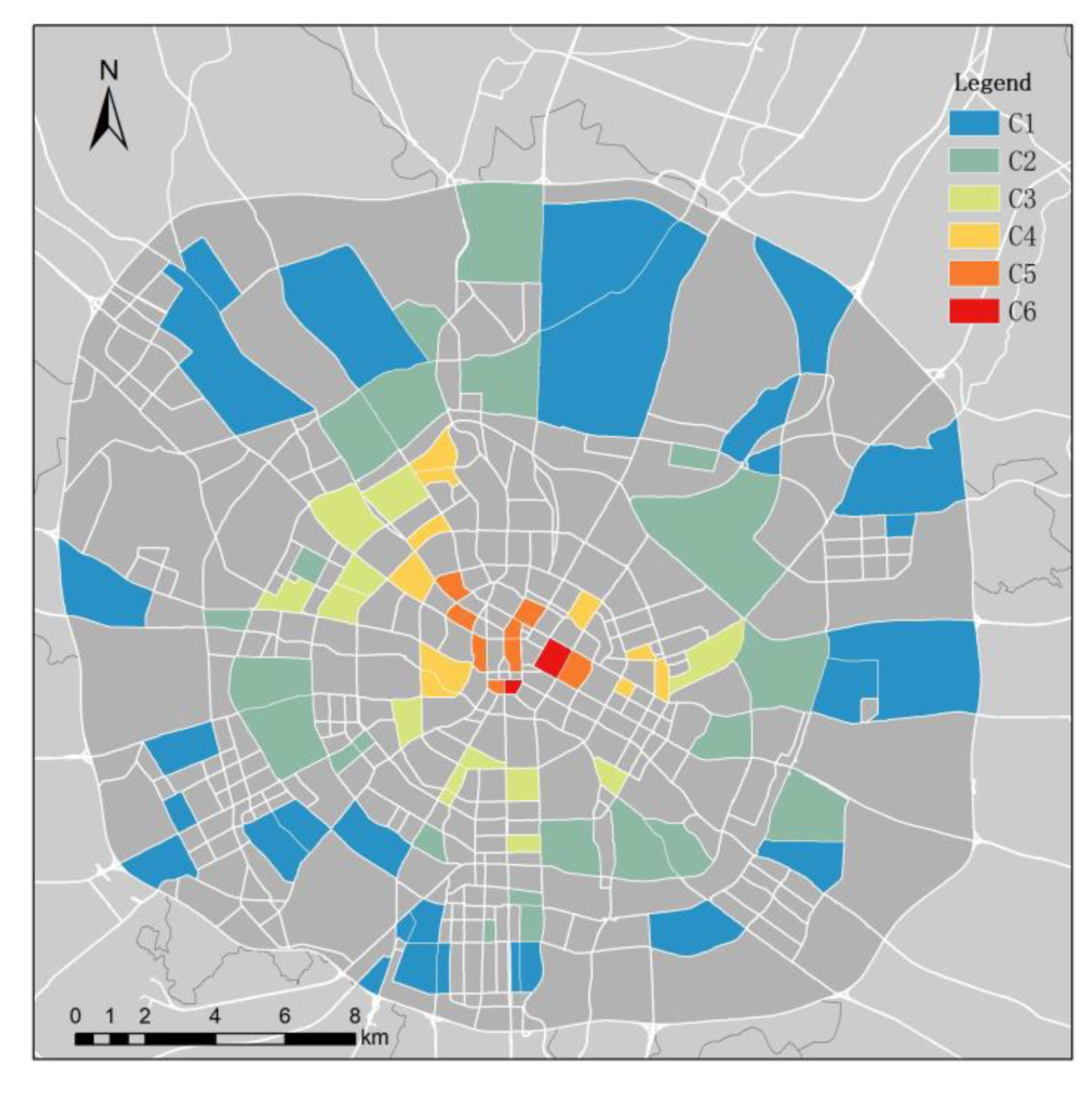
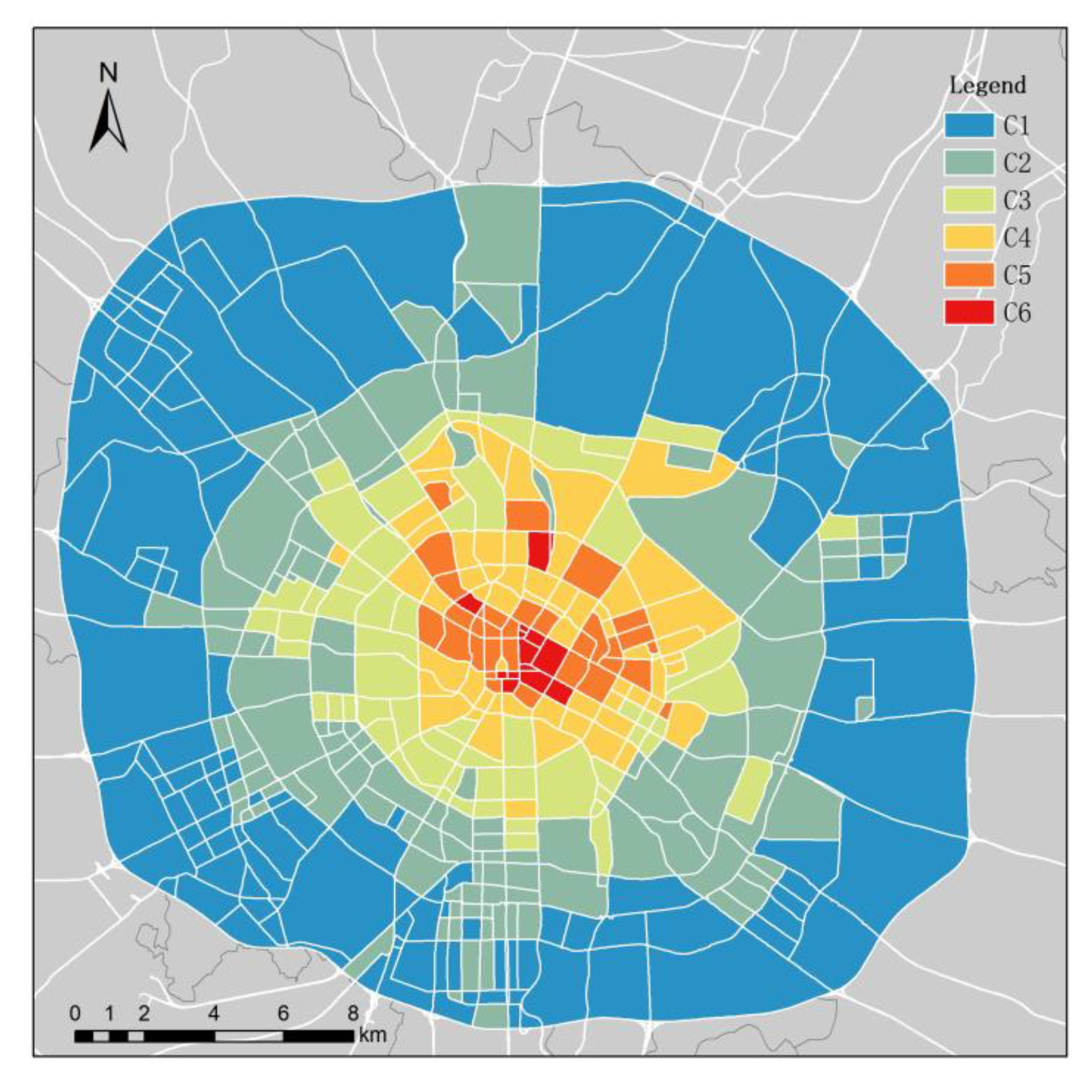
3.2. Results of KN–-DTW Classification

The above classification results of functional regions are obtained by direct K-medoid clustering of time series data. Direct clustering is an unsupervised learning method that may lead to inaccurate classification in some regions. To make the results more reliable, this study selected some data with good classification effects from the above clustering results as training samples according to the baselines of the time series of each cluster (Figure 7). KNN–DTW classification based on the training samples was then conducted on the remaining data to obtain the final result of the functional area classification (Figure 8). The baselines of the time series of each cluster can be used to obtain traffic volume and inflow information per unit time and area on working days and rest days to determine the travel patterns of residents in various plots (Figure 9).

3.3. Results of POI Auxiliary Analysis

To define the specific functions of each cluster, this study calculated the frequency density (FD) and category ratio (CR) of POI data of Cluster C1 to Cluster C6 (

Table 1. POI frequency density and category ratio in different clusters.

Category of POIs	C1			C2			C3
	$\mathit{F}\mathit{D}$	$\mathit{F}{\mathit{D}}_{\mathit{n}\mathit{o}\mathit{r}}$	$\mathit{C}\mathit{R}$	$\mathit{F}\mathit{D}$	$\mathit{F}{\mathit{D}}_{\mathit{n}\mathit{o}\mathit{r}}$	$\mathit{C}\mathit{R}$	$\mathit{F}\mathit{D}$	$\mathit{F}{\mathit{D}}_{\mathit{n}\mathit{o}\mathit{r}}$	$\mathit{C}\mathit{R}$
Catering	25.41	0.00	-	75.82	0.12	9.99%	138.49	0.27	9.04%
Shopping services	21.78	0.00	-	54.68	0.24	20.57%	64.31	0.32	10.72%
Leisure services	20.75	0.00	-	56.50	0.12	10.09%	109.16	0.30	10.06%
Accommodation	3.85	0.00	-	15.25	0.05	4.15%	26.75	0.10	3.36%
Science & Education	8.26	0.00	-	26.39	0.14	11.46%	59.72	0.39	13.12%
Healthcare services	9.75	0.00	-	25.02	0.16	13.45%	56.46	0.49	16.58%
Dwellings	6.33	0.00	-	20.34	0.09	7.29%	59.84	0.33	11.22%
Companies	27.41	0.00	-	64.91	0.10	8.25%	98.52	0.19	6.30%
Government agencies	6.05	0.00	-	14.16	0.09	7.70%	33.45	0.31	10.50%
Tourist attractions	0.73	0.00	-	1.51	0.08	7.04%	3.24	0.27	9.10%
Category of POIs	C4			C5			C6
	$\mathit{F}\mathit{D}$	$\mathit{F}{\mathit{D}}_{\mathit{n}\mathit{o}\mathit{r}}$	$\mathit{C}\mathit{R}$	$\mathit{F}\mathit{D}$	$\mathit{F}{\mathit{D}}_{\mathit{n}\mathit{o}\mathit{r}}$	$\mathit{C}\mathit{R}$	$\mathit{F}\mathit{D}$	$\mathit{F}{\mathit{D}}_{\mathit{n}\mathit{o}\mathit{r}}$	$\mathit{C}\mathit{R}$
Catering	165.72	0.33	8.94%	274.55	0.59	9.22%	450.62	1.00	10.36%
Shopping services	58.16	0.27	7.31%	88.19	0.49	7.75%	156.60	1.00	10.36%
Leisure services	122.73	0.34	9.25%	184.30	0.55	8.62%	319.49	1.00	10.36%
Accommodation	42.91	0.17	4.58%	92.83	0.38	6.05%	235.17	1.00	10.36%
Science & Education	61.63	0.40	10.85%	107.27	0.74	11.69%	141.54	1.00	10.36%
Healthcare services	71.84	0.65	17.58%	105.46	1.00	15.74%	72.55	0.66	6.79%
Dwellings	67.59	0.38	10.25%	126.73	0.74	11.70%	168.37	1.00	10.36%
Companies	124.85	0.25	6.89%	188.30	0.42	6.61%	410.65	1.00	10.36%
Government agencies	43.30	0.42	11.38%	89.86	0.95	14.88%	94.72	1.00	10.36%
Tourist attractions	5.23	0.48	12.97%	5.35	0.49	7.74%	10.13	1.00	10.36%

Note: In C1, due to the small number of points-of-interest (POIs) of all kinds, the value of $F{D}_{nor}$ is 0, so the value of $CR$ is meaningless when the denominator is 0.

). By analysing the residents’ travel characteristics and POI distribution characteristics of each cluster, the specific functions can be defined as follows.

C1 is distributed at the edge of the study area, and the frequency density of POIs is the lowest, so the rule should be determined by the direction of residents’ travel characteristics. Figure 9a shows that the population flow in this area is not obvious on weekdays. However, on rest days, the population inflow occurs in the morning, and there are relatively high population outflows in the afternoon and evening, which is consistent with the pattern of people playing and visiting relatives in suburban areas on weekends. Therefore, C1 is judged as the suburban tourism area.

C2 and C3 are distributed in the transition area between the suburb and the city. In terms of the proportion of POI types, both C2 and C3 have service facilities such as shopping, science, education and medical treatment necessary for residents’ lives, and C3 has relatively more residential POIs. In terms of travel characteristics, the outflow and inflow peaks of C2 on working days are 8:00 and 24:00, respectively; these peaks are at 8:00 and 19:00, respectively, in C3. Compared with C3 on working days, C2 has more obvious commuting patterns in residential areas. C2 belongs to the transitional region of C1 and C3, so it is determined that C3 is the urban residential area and C2 is the residential/tourism mixed area.

POIs in the office class (including science and education, medical treatment, corporations and government agencies) have high proportions of C4 and C5 compared with other areas. From the perspective of travel rules, C4 during the daytime (7:00–19:00) on working days experiences population outflow. The cut-off point for population inflow/outflow on the rest day is 13:00. The peak population outflow on the rest day occurs at 8:00. The traffic volume of C5 fluctuates frequently in a day, generating many extreme values. After 8:00 on weekdays, the inflow of the population gradually begins, while the outflow of the population reaches its peak at 18:00. Compared with C4, C5 has more obvious characteristics of commuting time, so it is judged as the office area. The characteristics of weekday population inflow in C4 are similar to those in residential areas, and the variation trends of the population inflow on rest days are the same as those on weekdays. However, the variation range is small, which may be because people′s shopping activities on rest days offset the original trend to some extent. Therefore, C4 is concluded to be the residential/commercial mixed area.

C6 is only distributed in the central area of the city. From the perspective of travel characteristics, the population inflow on weekends and weekdays reaches a peak at approximately 10:00, but the population outflow starts at 11:00 on rest days and 16:00 on working days. The traffic volume on rest days and working days peaks at 10:00 and 18:00, respectively, which is highly similar to people′s shopping times. According to the distribution characteristics of POIs, there are many types and quantities of POIs in this area, and all types of facilities are high-quality, so this area is judged to be the mature business area.

4. Discussion

In this paper, trajectory data were converted into time series data, and information mining was performed. After the similarity of the time series was obtained using the DTW calculation method, K-medoid clustering was performed, and the results with good clustering effects were selected as the training samples. Then, KNN classification was performed based on the training samples to obtain the final identification of urban functional areas. This study can provide a new idea for data classification without training samples. Although the method is common, it is very suitable for machine learning of trajectory time series. As long as this idea is followed, replacing K-medoids and KNN with other methods is also suitable for big data mining.

To verify the identification effect of this method, the results were compared with Google Earth images, Gaode Maps, and real photos of landmark areas. The comparison results in some typical regions are shown in

Table 2. Comparison and evaluation of functional area identification results.

Functional Area	No.	Results of Identification	Google Earth Image	Gaode Map (English Edition)	Real Photos of Landmark Site
C1: Suburban Tourism Area	1		Lat.: 30.637492 Lon.: 104.178509	Lat.: 30.634418 Lon.: 104.181086	Date: 2018/9/6
	2		Lat.: 30.751676 Lon.: 104.137462	Lat.: 30.746165 Lon.: 104.136454	Date: 2017/12/30
C2: Residential/Tourism Mixed Area	3		Lat.: 30.729891 Lon.: 104.031037	Lat.: 30.729678 Lon.: 104.035385	Date: 2019/6/21
	4		Lat.: 30.616207 Lon.: 104.083512	Lat.: 30.614217 Lon.: 104.086004	Date: 2017/8/31
C3: Urban Residential Area	5		Lat.: 30.636909 Lon.: 104.039137	Lat.: 30.634067 Lon.: 104.042427	Date: 2016/5/23
	6		Lat.: 30.650295 Lon.: 104.025001	Lat.: 30.648028 Lon.: 104.027046	Date: 2016/9/16
C4: Residential/Commercial Mixed Area	7		Lat.: 30.656678 Lon.: 104.053936	Lat.: 30.648305 Lon.: 104.047764	Date: 2017/4/17
	8		Lat.: 30.656678 Lon.: 104.053936	Lat.: 30.655058 Lon.: 104.056887	Date: 2017/2/12
C5: Office Area	9		Lat.: 30.654412 Lon.: 104.070917	Lat.: 30.652455 Lon.: 104.073602	Date: 2018/7/6
	10		Lat.: 30.669699 Lon.: 104.090741	Lat.: 30.667969 Lon.: 104.092903	Date: 2017/4/17
C6: Mature Business Area	11		Lat.:30.658748 Lon.:104.072673	Lat.: 30.656309 Lon.: 104.075811	Date: 2017/1/20
	12		Lat.:30.659761 Lon.:104.063428	Lat.: 30.657511 Lon.: 104.065741	Date: 2018/2/9

. The data below the Google image and the Gaode Map image are the locations (latitude and longitude) of the centre point of the captured image. Since the reference coordinate system of Google Earth and Gaode Map are different, there will be some deviation in the dimension and longitude data of the same spot. In addition, to get as close as possible to the time of the trajectory data and POI data, Google images of 2017/4/13 was selected. The capture time of the Gaode Map was 2019/8/17. The fetch time of real photos varied from place to place, so the fetch time is marked below the image in Table 2.

The landmark area in the first group is Qinglong Wetland Park, which is the largest wetland park and a famous historical and cultural scenic spot in Chengdu. The second group is the Chengdu Research Base of Giant Panda Breeding, a famous institution for giant panda research, breeding and protection in China and the world; it is also a national AAAA tourist attraction. As famous tourist attractions, these areas are in line with the urban functions of suburban tourism. In the third and fourth groups, the landmark areas are Chengdu Happy Valley and East Lake Park, which are also famous scenic spots in Chengdu city. However, in these areas, in addition to tourist attractions, there are some moderately dense residential buildings. In groups 5 and 6, a large number of residential buildings with high density and orderly arrangement are distributed. Furthermore, this area is close to the city centre, which is consistent with the positioning of the “Urban Residential Area” functional area. From the comparison of groups 1–6, it can be found that the living, travelling and transition areas can be well separated in this study.

The area in group 7 is Jinli, which contains a variety of specialty food and beverage shops and themed commodity shops with prominent commercial functions. There are also some residential buildings similar to those in C3 in this area. The area in the eigth group is People′s Park, which is the centre of the old city of Chengdu. Although this area has certain tourist value, the distribution of old shops with strong histories and low, densely populated old houses around the area is more prominent. In summary, both of these areas are in line with their location in the “Residential/Commercial Mixed Area”. The landmarks in groups 9 and 10 are the People′s Government of Sichuan Province and the Chengdu 339 TV Tower, which not only have prominent office functions but are also well supplemented by a large number of office buildings distributed around them. The landmark area in the 11th group is Chunxi Road, which is the busiest and most prosperous commercial street in Chengdu and the characteristic commercial street that is famous in literature all over the country. The area in the 12th group is Tianfu Square, which is located in central Chengdu city. This area has consistently been the symbol of Chengdu and even Sichuan Province, and it is a city landmark. These two areas are located in the centre of the city, where commercial functions occupy almost the entire area. There are few buildings for other functions around them, so they are in line with the functional positioning of “Mature Commercial Areas”.

The comparison of groups 7–12 reveals that this study has a good ability to distinguish mature commercial areas from residential/commercial areas. The distribution of office areas is similar to the two adjacent functional areas, but the functions are quite different. This study can also identify these patterns.

In summary, the method used in this study can effectively identify the main functions and their distribution in Chengdu city with good accuracy. According to the identification results, the distribution of functional areas in the study area is basically circular and follows the distribution mode of tourism–residence–commerce, which is consistent with the generally recognized urban structure of Chengdu.

In a recent study of Chengdu urban functional regions, the research by Gao et al. [37] was also based on trajectory data and adopted a combination of Gaussian mixture model (GMM) and Pearson correlation coefficient (PCC). Their results are similar to the results of this study, although there are some differences in the nomenclature and regional definitions of functional areas; however, there are few differences in the overall urban functions and their distribution. In addition, Gao’s results can distinguish Chunxi Road and Chengdu Railway Station from other functional areas and identify them separately, which is not achieved by the method in this paper. These two sites are relatively single and prominent, so this point has reference value for this paper. The training sample selection method used in this paper and the idea of semi-supervised learning also have reference value for the data mining models using clustering alone.

5. Conclusions

With the deepening of urbanization, the spatial structures of cities present complex but regular characteristics. This paper analyses the urban spatial structure from the perspective of big data mining. The results of this method are consistent with the actual situation, and the findings of this study are as follows. Traffic volume and inflow can better reflect residents’ travel rules than simple on and off data. The original DTW method has high temporal complexity, which can be improved by normalization and the reduction of the dimensionality of the time series. The semi-supervised learning classification method is applicable to trajectory data, and it is better to select typical unsupervised learning models as the training samples. This method can provide a theoretical basis for urban land planning, administrative division adjustments, urban resource allocation and other fields, and it has auxiliary and guiding value for the overall scientific planning of land use and urbanization layout in the context of national spatial planning policies in the new era.

There is still much work to be done in this area of study in the future. In this paper, taxis are taken as representative of residents’ travel, and other means of residents’ travel, such as public transportation and bicycles, are not considered. In addition, LBS big data, such as WeChat circle of friends data and Weibo check-in data, have important reference value for the interpretation and classification of urban land use. Therefore, multi-source urban big data should be integrated in future studies to make the classification results more detailed and reliable. In addition, after obtaining reliable classification results of urban functional areas, the spatial structure of each functional area and its correlation degree can be analysed. Then, the reasonable utilization degree of urban space can be evaluated to attempt to provide effective optimization suggestions.

References

1. Gao, S.; Janowicz, K.; Couclelis, H. Extracting urban functional regions from points of interest and human activities on location-based social networks. Trans. GIS 2017, 21, 446–467. [Google Scholar] [CrossRef]
2. Wang, H.; Pingping, T.; Liu, H. Spatial structuring of the ‘new economies’ in xi’an and its mechanisms. Geogr. Res. 2006, 3, 173–184. [Google Scholar]
3. Herold, M.; Couclelis, H.; Clarke, K.C. The role of spatial metrics in the analysis and modeling of urban land use change. Comput. Environ. Urban Syst. 2005, 29, 369–399. [Google Scholar] [CrossRef]
4. Banzhaf, E.; Netzband, M. Monitoring urban land use changes with remote sensing techniques. In Applied Urban Ecology: A Global Framework; John Wiley & Sons, Ltd: Hoboken, NJ, USA, 2011. [Google Scholar]
5. Barnsley, M.J.; Barr, S.L. Inferring urban land use from satellite sensor images using kernel-based spatial reclassification. Photogramm. Eng. Remote Sens. 1996, 62, 949–958. [Google Scholar]
6. Ahas, R.; Mark, Ü. Location based services—New challenges for planning and public administration? Futures 2005, 37, 547–561. [Google Scholar] [CrossRef]
7. Ratti, C.; Pulselli, R.M.; Williams, S.; Frenchman, D. Mobile landscapes: Using location data from cell phones for urban analysis. Environ. Plan. B Plan. Des. 2006, 33, 727–748. [Google Scholar] [CrossRef]
8. Joh, C.; Hwang, C. A time-geographic analysis of trip trajectories and land use characteristics in seoul metropolitan area by using multidimensional sequence alignment and spatial analysis. In Proceedings of the AAG Annual Meeting, Washington, DC, USA, 14–17 April 2010. [Google Scholar]
9. Kling, F.; Pozdnoukhov, A. When a city tells a story:Urban topic analysis. In Proceedings of the International Conference on Advances in Geographic Information Systems, Redondo Beach, CA, USA, 6–9 November 2012. [Google Scholar]
10. Steiger, E.; Westerholt, R.; Zipf, A. Research on social media feeds–A giscience perspective. In European Handbook of Crowdsourced Geographic Information; Ubiquity Press: London, UK, 2016; Volume 99, pp. 237–254. [Google Scholar]
11. Dong, M. Research on Identifying Urban Regions of Different Functions from Wechat Data and Pois. Master’s Thesis, Zhejiang Normal University, Jinhua, China, 2017. [Google Scholar]
12. Phithakkitnukoon, S.; Horanont, T.; Lorenzo, G.D.; Shibasaki, R.; Ratti, C. Activity-aware map: Identifying human daily activity pattern using mobile phone data. In Human Behavior Understanding, First International Workshop; Springer: Berlin/Heidelberg, Germany, 2010. [Google Scholar]
13. Soto, V.; Frías-Martínez, E. Automated land use identification using cell-phone records. In Proceedings of the Acm International Workshop on Mobiarch, Washington, DC, USA, 28 June–1 July 2011. [Google Scholar]
14. Becker, R.A.; Cáceres, R.; Hanson, K.; Ji, M.L.; Volinsky, C. A tale of one city: Using cellular network data for urban planning. IEEE Pervasive Comput. 2011, 10, 18–26. [Google Scholar] [CrossRef]
15. Brockmann, D.; Theis, F.J. Money circulation, trackable items, and the emergence of universal human mobility patterns. IEEE Pervasive Comput. 2008, 7, 28–35. [Google Scholar] [CrossRef]
16. Doyle, J.; Hung, P.; Farrell, R.; McLoone, S. Population mobility dynamics estimated from mobile telephony data. J. Urban Technol. 2014, 21, 109–132. [Google Scholar] [CrossRef]
17. Yuan, J.; Zheng, Y.; Xie, X. Discovering regions of different functions in a city using human mobility and pois. In Proceedings of the Acm Sigkdd International Conference on Knowledge Discovery & Data Mining, Beijing, China, 12–16 August 2012. [Google Scholar]
18. Sun, L.; Lee, D.H.; Erath, A.; Huang, X. Using smart card data to extract passenger′s spatio-temporal density and train′s trajectory of mrt system. In Proceedings of the Acm Sigkdd International Workshop on Urban Computing, Beijing, China, 12 August 2012. [Google Scholar]
19. Zhong, C.; Huang, X.; Arisona, S.M.; Schmitt, G.; Batty, M. Inferring building functions from a probabilistic model using public transportation data. Comput. Environ. Urban Syst. 2014, 48, 124–137. [Google Scholar] [CrossRef]
20. Han, H.; Yu, X.; Long, Y. Discovering functional zones using bus smart card data and points of interest in beijing. In City Planning Review; Springer: Cham, Germany, 2015. [Google Scholar]
21. Mckenzie, G.; Janowicz, K.; Gao, S.; Gong, L. How where is when? On the regional variability and resolution of geosocial temporal signatures for points of interest. Comput. Environ. Urban Syst. 2015, 54, 336–346. [Google Scholar] [CrossRef]
22. Yu, L.; Wang, F.; Xiao, Y.; Gao, S. Urban land uses and traffic ‘source-sink areas’: Evidence from gps-enabled taxi data in shanghai. Landsc. Urban Plan. 2012, 106, 73–87. [Google Scholar]
23. Pan, G.; Qi, G.; Wu, Z.; Zhang, D.; Li, S. Land-use classification using taxi gps traces. Intell. Transp. Syst. IEEE Trans. 2013, 14, 113–123. [Google Scholar] [CrossRef]
24. Chen, S.; Tao, H.; Li, X.; Zhuo, L. Discovering urban functional regions using latent semantic information: Spatiotemporal data mining of floating cars gps data of guangzhou. Acta Geogr. Sin. 2016, 71, 471–483. [Google Scholar]
25. Cheng, J.; Liu, J.; Gao, Y. Analyzing the spatio-temporal characteristics of beijing′s od trip volume based on time series clustering method. J. Geo Inf. Sci. 2016, 18, 1227–1239. [Google Scholar]
26. Mori, U.; Mendiburu, A.; Lozano, J.A. Similarity measure selection for clustering time series databases. IEEE Trans. Knowl. Data Eng. 2015, 28, 181–195. [Google Scholar] [CrossRef]
27. Li, Z.; Zhao, Y.; Liu, R.; Pei, D. Robust and rapid clustering of kpis for large-scale anomaly detection. In Proceedings of the 2018 IEEE/ACM 26th International Symposium on Quality of Service, IWQoS, Banff, AB, Canada, 4–6 June 2018; pp. 1–10. [Google Scholar]
28. Shokoohi-Yekta, M.; Hu, B.; Jin, H.; Wang, J.; Keogh, E. Generalizing dtw to the multi-dimensional case requires an adaptive approach. Data Min. Knowl. Discov. 2017, 31, 1–31. [Google Scholar] [CrossRef] [Green Version]
29. Ma, C.H.; Weng, X.Q.; Shan, Z.N. Early classification of multivariate time series based on piecewise aggregate approximation. In Computer Science; Springer: Cham, Germany, 2017. [Google Scholar]
30. Cheng, W.; Zou, P.; Jia, Y.; Yang, Y. Anomaly detection over pseudo period data streams based on dtw distance. J. Comput. Res. Dev. 2010, 47, 893–902. [Google Scholar]
31. Zhu, X.; Goldberg, A.B. Introduction to Semi-Supervised Learning; Morgan & Claypool: Williston, VT, USA, 2009. [Google Scholar]
32. Chen, Y.; Liu, X.; Li, X.; Liu, X.; Yao, Y.; Hu, G.; Xu, X.; Pei, F. Delineating urban functional areas with building-level social media data: A dynamic time warping (dtw) distance based k -medoids method. Landsc. Urban Plan. 2017, 160, 48–60. [Google Scholar] [CrossRef]
33. Zhu, C.; Cheng, G.; Wang, K. Big data analytics for program popularity prediction in broadcast tv industries. IEEE Access 2017. [Google Scholar] [CrossRef]
34. Costa, B.G.; Freire, J.C.A.; Cavalcante, H.S.; Homci, M.; Castro, A.R.G.; Viegas, R.; Meiguins, B.S.; Morais, J.M. Fault classification on transmission lines using knn-dtw. In Proceedings of the International Conference on Computational Science & Its Applications, Trieste, Italy, 3–6 July 2017. [Google Scholar]
35. Hsu, H.-H.; Yang, A.C.; Lu, M.-D. Knn-dtw based missing value imputation for microarray time series data. J. Comput. 2011, 6, 418–425. [Google Scholar] [CrossRef]
36. Mitsa, T. Temporal Data Mining; CRC: Boca Raton, FL, USA, 2010. [Google Scholar]
37. Qingke, G.; Jianhong, F.; Yang, Y.; Xuehua, T. Identification of urban regions’ functions in Chengdu, China, based on vehicle trajectory data. PLoS ONE 2019, 14. [Google Scholar] [CrossRef] [Green Version]
38. Liu, J.; Xu, J.; Cai, L.; Meng, B.; Pei, T. Identifying functional regions based on the spatio-temporal pattern of taxi trajectories. J. Geo Inf. Sci. 2018, 20, 1550–1561. [Google Scholar]
39. Chen, Z.; Qiao, B.; Zhang, J. Identification and spatial interaction of urban functional regions in beijing based on the characteristics of residents’ traveling. J. Geo Inf. Sci. 2018, 20, 291–301. [Google Scholar]
Figure 1. Study Area. The administrative division data are from the National Geomatics Center of China (http://www.ngcc.cn/ngcc/), and the research area is within the beltway of Chengdu.
Ijgi 09 00158 g001
Figure 2. Traffic analysis zones. Traffic analysis zones were obtained by cutting study area with main roads network, and they were taken as the basic spatial unit in this study.
Ijgi 09 00158 g002
Figure 3. Flow chart of the research. The figure shows the process of urban functional areas identification based on taxi trajectory data and POI data, including the generation of time series, K-medoids clustering, selection of training samples and k-nearest neighbour classification.
Ijgi 09 00158 g003
Figure 4. Characteristics of resident trips in the study area. (a) quantity of pickups/drop-offs on workdays/weekends. A represents the quantity of pickups on workdays; B represents the number of pickups on weekends; C represents the quantity of drop-offs on workdays; D represents the quantity of drop-offs on weekends; (b) quantity of traffic volume/inflow on workdays/weekends. E represents the traffic volume on workdays; F represents the traffic volume on weekends; G represents the inflow on workdays; H represents the inflow on weekends.
Ijgi 09 00158 g004
Figure 5. The changes in silhouette values with different numbers of cluster. Silhouette coefficient was calculated by repeating clustering operations, and the larger the silhouette value is, the better the clustering effect will be.
Ijgi 09 00158 g005
Figure 6. The results of K-medoids. Based on the trajectory time series data, the land is divided into six clusters (C1~C6), but the specific functions of each cluster are still unknown.
Ijgi 09 00158 g006
Figure 7. Selections for training samples. The baseline of the time series of each cluster was taken as the evaluation standard, and data with good clustering effects of 20% were selected as the training samples.
Ijgi 09 00158 g007
Figure 8. The results of k-nearest-neighbor–dynamic-time-warping (KNN¬–DTW).KNN-DTW classification based on the training samples was conducted on the remaining data to obtain the final result of the functional area classification.
Ijgi 09 00158 g008
Figure 9. Characteristics of resident trips in different clusters. (a) tTraffic volume/inflow quantity on workdays/weekends per square kilometre in Cluster 1. (b) Traffic volume/inflow quantity on workdays/weekends per square kilometre in Cluster 2. (c) Traffic volume/inflow quantity on workdays/weekends per square kilometre in Cluster 3. (d) Traffic volume/inflow quantity on workdays/weekends per square kilometre in Cluster 4. (e) Traffic volume/inflow quantity on workdays/weekends per square kilometre in Cluster 5. (f) Traffic volume/inflow quantity on workdays/weekends per square kilometre in Cluster 6.
Ijgi 09 00158 g009aIjgi 09 00158 g009b