FloodSim: Flood Simulation and Visualization Framework Using Position-Based Fluids


Department of Computing Sciences, Texas A&M University—Corpus Christi, Corpus Christi, TX 78412, USA
*
Author to whom correspondence should be addressed.
ISPRS Int. J. Geo-Inf. 2020, 9(3), 163; https://0-doi-org.brum.beds.ac.uk/10.3390/ijgi9030163
Submission received: 18 February 2020
/
Revised: 6 March 2020
/
Accepted: 7 March 2020
/
Published: 11 March 2020
Abstract
:Flood modeling and analysis has been a vital research area to reduce damages caused by flooding and to make urban environments resilient against such occurrences. This work focuses on building a framework to simulate and visualize flooding in 3D using position-based fluids for real-time flood spread visualization and analysis. The framework incorporates geographical information and takes several parameters in the form of friction coefficients and storm drain information, and then uses mechanics such as precipitation and soil absorption for simulation. The preliminary results of the river flooding test case were satisfactory, as the flood extent was reproduced in 220 s with a difference of 7%. Consequently, the framework could be a useful tool for practitioners who have information about the study area and would like to visualize flooding using a particle-based approach for real-time particle tracking and flood path analysis, incorporating precipitation into their models.
1. Introduction
Flood modeling and analysis has been a vital research area to reduce damages caused by flooding and to assess urban environment resilience against such occurrences [1,2,3]. 2D and 3D hydrodynamic models have been used to provide insight to practitioners and city planners to determine patterns, risks, and anomalies in the environment through visualization of the phenomena. To accomplish a realistic simulation, the environment must be defined accurately, and local dynamics must be realized to analyze such events.
Historical information is a vital resource in flood modeling and analysis, and can contain valuable insight for the study area [4]. Although the availability of such information might be problematic, if historical information about a region is found, then flood risk analysis can be performed [5]. Geologic evidence and past stream gauge data left behind due to the occurrence of large floods enable researchers to collect and process information to analyze flood data [4]. However, many floods are not included in the written history, and consequently it is challenging and expensive to search for historical evidence to assess flooding [6]. Empirical methods have been investigated to model flooding and how the local dynamics direct or divert flooding [7,8]. These observations can be utilized in emergency management scenarios to support decision making [9,10]. As empirical flood modeling focuses on the formulation of certain properties of water, it is important to collect sufficient information regarding the study area to be able to provide values to the system. Maximum flood discharge, rainfall intensity, catchment area, and certain coefficients specific to the area being investigated are significant parameters for such formulas. Especially with the prominence of 1D and 2D hydrodynamic simulations to simulate flooding, empirical models can provide a level of correctness to other models [11].
Hydrodynamic models utilize a mathematical approach to solve a variety of equations depending on the domain to represent the physical behavior of flooding or waters. 1D and 2D models have been used in analyzing and modeling flash floods [12,13], decision support systems [9], and hydrodynamic modeling [14]. 2D models have been used in the research community for their accuracy in solving full shallow water equations [6]. By describing an additional dimension, these models are better in describing the flood progression and diffusion compared to 1D simulations. Through the advancement of modern graphics processing units (GPUs), 2D and 3D visualization have been utilized in flood modeling and analysis. Teng et al. [6] introduce empirical, hydrodynamic, and simplified methods used in flood modeling and underline that hydrodynamic models utilizing 2D and 3D simulations may prove to be better in representing detailed flow dynamics. Furthermore, simplified models can be used best for probabilistic flood risk assessment. Leskens et al. [15] present a system for analyzing flooding scenarios through 3D visualization. Upon representing the virtual environment, numerical methods that solve 2D hydraulic equations for water flow are used to simulate the flood. Note that 3D representation of the flood helps practitioners to better realize and estimate the impact of a flood. 2D and 3D models have been used for storm surge flood routing visualization [16], risk estimation [17], flood modeling and analysis [15,18,19], rainfall forecasting [20], landslide simulation [21], and to visualize many other scenarios. Recent works show a move from static visualization to dynamic visualization [22,23,24], to provide more interactive and accessible simulation tools to incorporate virtual environments and dynamic simulation parameters.
There are numerous software packages that offer a collection of models to represent a specialized aspect of flooding. The Hydrologic Engineering Center’s River Analysis System (HEC-RAS) is a numerical model featuring an integrated 1D model to represent flow, and provides an interactive environmental management scenario [25]. It has commonly been used for evaluating and visualizing river dynamics through performing 1D steady and 2D unsteady river flow calculations to estimate flooding [26], and has been utilized for the prediction of flood extent, simulation of overland flow, and examination of large floodplains [27,28,29]. Similar to HEC-RAS, MIKE FLOOD is unique software providing a coupled 1D–2D hydrodynamic model [30] suitable for modeling and accomplishing flood forecasting, flood management, flood risk analysis and hazard mapping, visualization, and evaluation of dam break scenarios and river and coastal flooding [31,32]. LISFLOOD-FP [33] is a 2D hydrodynamic model which excels in visualizing and processing flood inundation efficiently for complex topographies, and it can be used for flood inundation prediction and flood risk assessment [34,35]. The existence and usability of these models show the importance of software tools and the need for alternative approaches and methods to investigate the phenomena.
Recently, with the improvements of modern GPUs and the availability of data, 3D simulations and especially particle-based Lagrangian simulations have been investigated in the literature [6]. Furthermore, recent research has attempted to alleviate the performance issues of particle-based simulation methods, making them feasible for interactive simulations [36,37]. Among methods used to simulate flooding, many works utilize smoothed particle hydrodynamics (SPH) [38,39]. Furthermore, position-based fluids (PBF) is designed with real-time performance in mind [40] and consequently, if it can describe the flood extent properly, then the method can be utilized in practical scenarios.
In this work, considering the state-of-the-art approaches discussed above, we built a Lagrangian flood simulation and visualization framework called FloodSim for realistic and efficient representation of the flooding phenomena. PBF [40] was utilized for simulating flood, which considers a Lagrangian description and provides benefits over traditional smoothed-particle hydrodynamics (SPH) [38] methods by providing stability [41] and alleviating the neighborhood requirement [40] of traditional SPH, which has an expensive computation of determining a particle’s neighborhood [36]. By utilizing an efficient flood simulation framework using position-based fluids, real-time performance is provided in a variety of scenarios. An urban environment reconstruction tool called City Maker [42], which was developed to be utilized alongside FloodSim, is used to generate 3D digital environment models. Through implementation of a local friction model, rainfall and cloud mechanics, and soil absorption mechanics, dynamic behavior to the environment is implemented, and an approximate description of the study area showing the extent of flooding is acquired.
2. Methodology
In this section, details about the flood simulation and visualization framework FloodSim are provided. Upon discussion of the overall system design, more details about the system are introduced in the following subsections. As the framework consists of multiple components to visualize the phenomena, subsections expand on these components and explain how these individual parts collaborate to provide an effective flood simulation.
2.1. System Overview
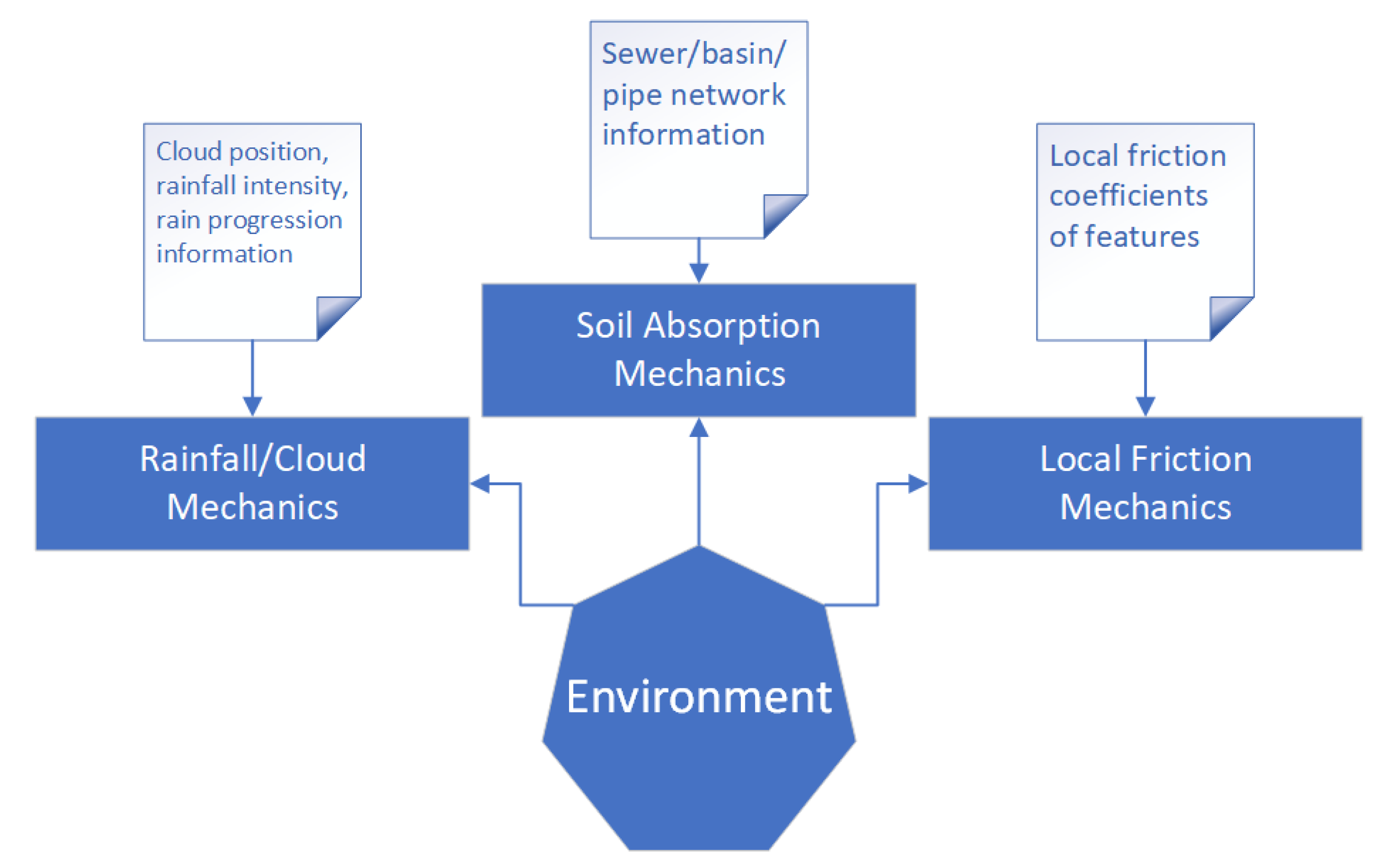
FloodSim, the simulation framework built for this study, contains several modules to accommodate various tasks. These modules are initialized to prepare the simulation engine for environmental parameter utilization, smooth fluid particle behavior, and animated rainfall. Figure 1 shows these FloodSim modules and required inputs for the system to be provided with critical information.
Position-based fluids [40] is used as the simulation method. As mentioned earlier, among the computational methods available to render and visualize fluids, position-based fluids is a recent but well-established method that is well optimized for real-time soft interactive simulations. As it is not a common architecture within the flood modeling community, it is worth emphasizing that FloodSim utilizes it to alleviate some common issues of SPH and to provide an engine which focuses on performance.
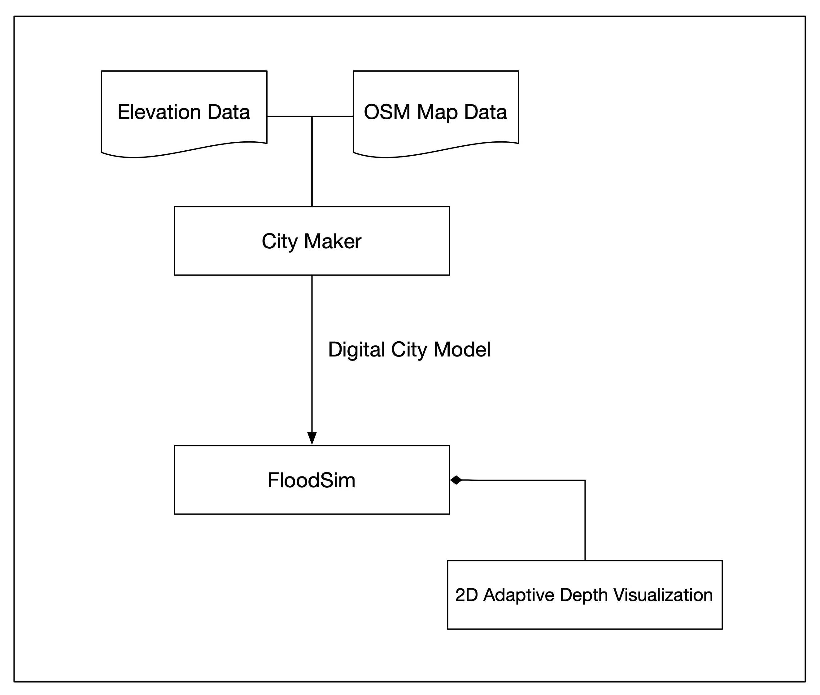
As indicated earlier, City Maker [42] is used to provide the digital environment model for the simulation environment. By parsing OpenStreetMap (OSM) data and extracting significant features, City Maker is flexible enough to provide the required GIS layers to the environment. Furthermore, a particle-based fluids visualization tool [43] is utilized to visualize the environment in 2D. Using this, clarity in otherwise complex-to-comprehend scenarios can be achieved. Figure 2 shows an overview of the workflow and how FloodSim is utilized alongside the tools discussed.
2.2. Global and Local Friction Model
Simulations require several important environmental parameters for the computations to be done accurately. Among these parameters, friction is vital. Objects are given a friction parameter that relates to the roughness of the surface, controlling how freely water flows over those surfaces. Additionally, friction between water particles is considered using viscous forces in the computations.
As part of the position-based fluids framework [40], two global friction coefficients for static and dynamic friction are provided to account for different scenarios. A static friction coefficient is considered for stable entities in the environment, while dynamic friction coefficients are utilized to define the behavior of moving fluid particles. With static friction, the stability of water particles can be achieved as the coefficient defines the behavior of the particles when they are not in motion. On the other hand, dynamic friction defines the interaction between the surface and the fluid as the particles are moving. However, these coefficients are global friction coefficients and do not define the behavior of different materials in the environment.
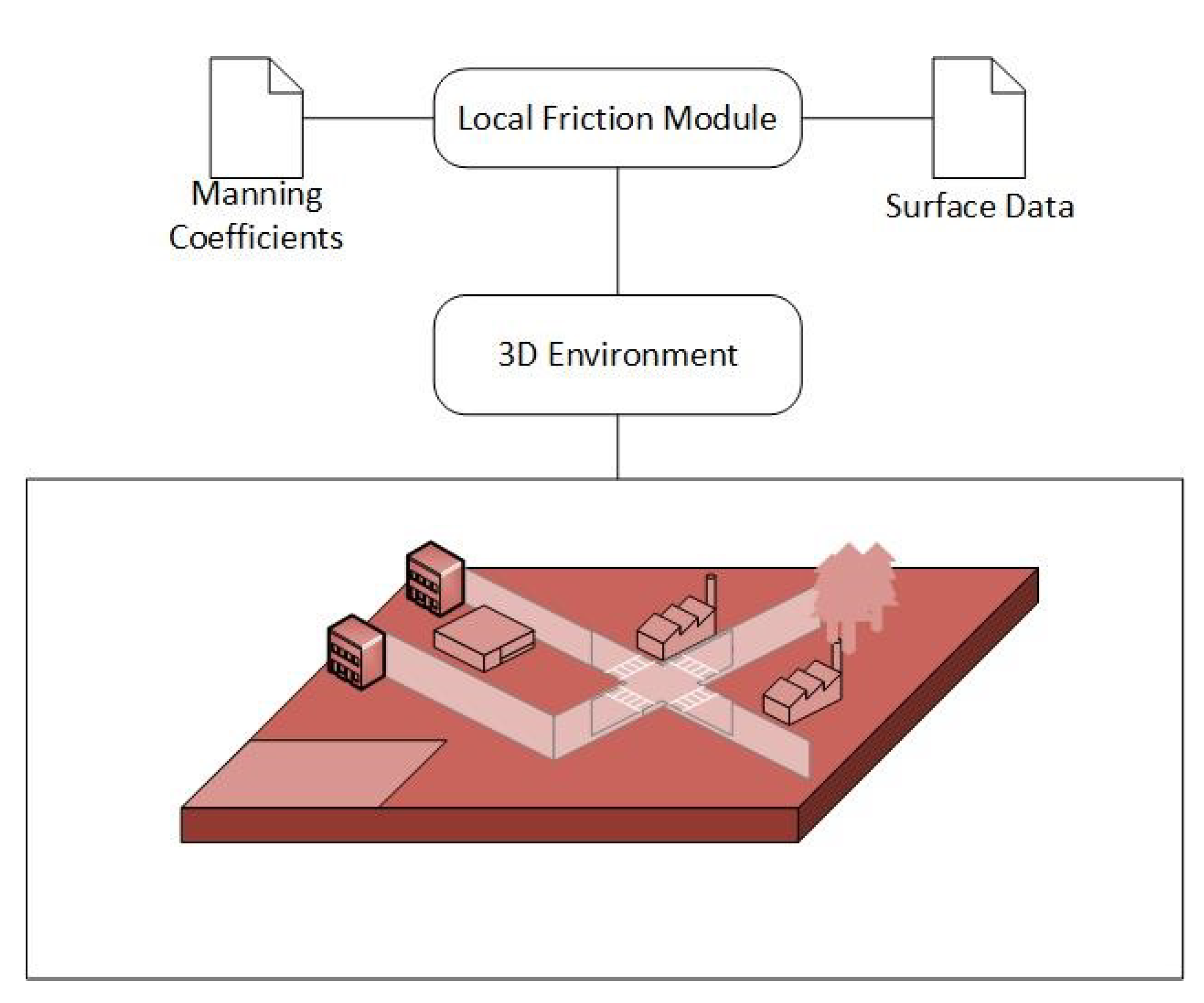
Various works underline that some utility of local friction coefficients are used to simulate flood flow [44,45,46], and consequently, our implementation is provided for the users to provide friction values for the features. As our domain is urban environments, differentiating between grasslands, farmlands, road networks, concrete, and any other significant material is imperative. Water flow and soil absorption works differently on different surfaces, and thus local friction coefficients are implemented to define this behavior. To enhance the global friction model with the local friction model, Manning coefficients [47] are utilized. Utilizing these values with the surface information coming from the flood visualization framework, coefficients are provided. As we focused on extracting the environment from OpenStreetMap data using City Maker [42], environmental information comes automatically. Nevertheless, if a user chooses to import a manually defined environment, then an appropriate file carrying contextual information must be provided. For this, our system reads environmental information alongside the Manning coefficients file to define areas in the environment with distinct friction parameters. By matching feature types with the values found in the coefficients file, roughness parameters are embedded into the digital model. This process is shown in Figure 3. In this figure, darker reds show higher friction coefficients while lighter reds indicate lower coefficients.
2.3. Soil Absorption Mechanics
An important component embedded into the simulation framework is the mechanics that define how soil absorption works within the environment. Considering other frameworks developed to visualize water translation, this feature is either left out intentionally or implemented with certain approximations. Although empirical models may utilize the real values for the soil type of the environment after a thorough survey of the region, experimental models such as SPH-based 3D fluid mechanics utilize alternative ways to compensate slower performance due to particle interaction. As underlined earlier, another approach is to leave this feature out if the experiment is about surface runoff simulations and environmental effects over some period are not being tracked.
In the context of this framework, soil absorption does not only refer to the terrain, soil type, and soil saturation, but also refers to the overall absorption of water through citywide stormwater drains. Therefore, FloodSim incorporates a soil absorption engine and expects additional data to simulate the drains. The side inlets and grated inlets are modeled according to the specifications provided by the city, if available. Upon modeling these inlets and placing them properly around the 3D environment, the soil absorption works by removing a certain number of particles per simulation second to represent inlets carrying water away. Consequently, it is vital to find the drain information of the study area. Furthermore, features placed in the environment and the terrain may have different local soil absorption coefficients for realistic behavior of flood waters. Therefore, for each feature drawn on the environment, a local absorption coefficient is provided for further accounting for the different types of soils the environment might have. For example, a park may have a higher intrinsic absorption value than a road. Each soil type contains a saturation level, and when it reaches 100%, absorption stops as the water is considered to be running off the surface. Evaporation is taken into account through an evaporation rate, which can be set up according to the environmental properties of the study area. By utilizing storm sewer data only, this behavior cannot be provided, and therefore a feature level absorption coefficient can be used for representing this absorption mechanic.
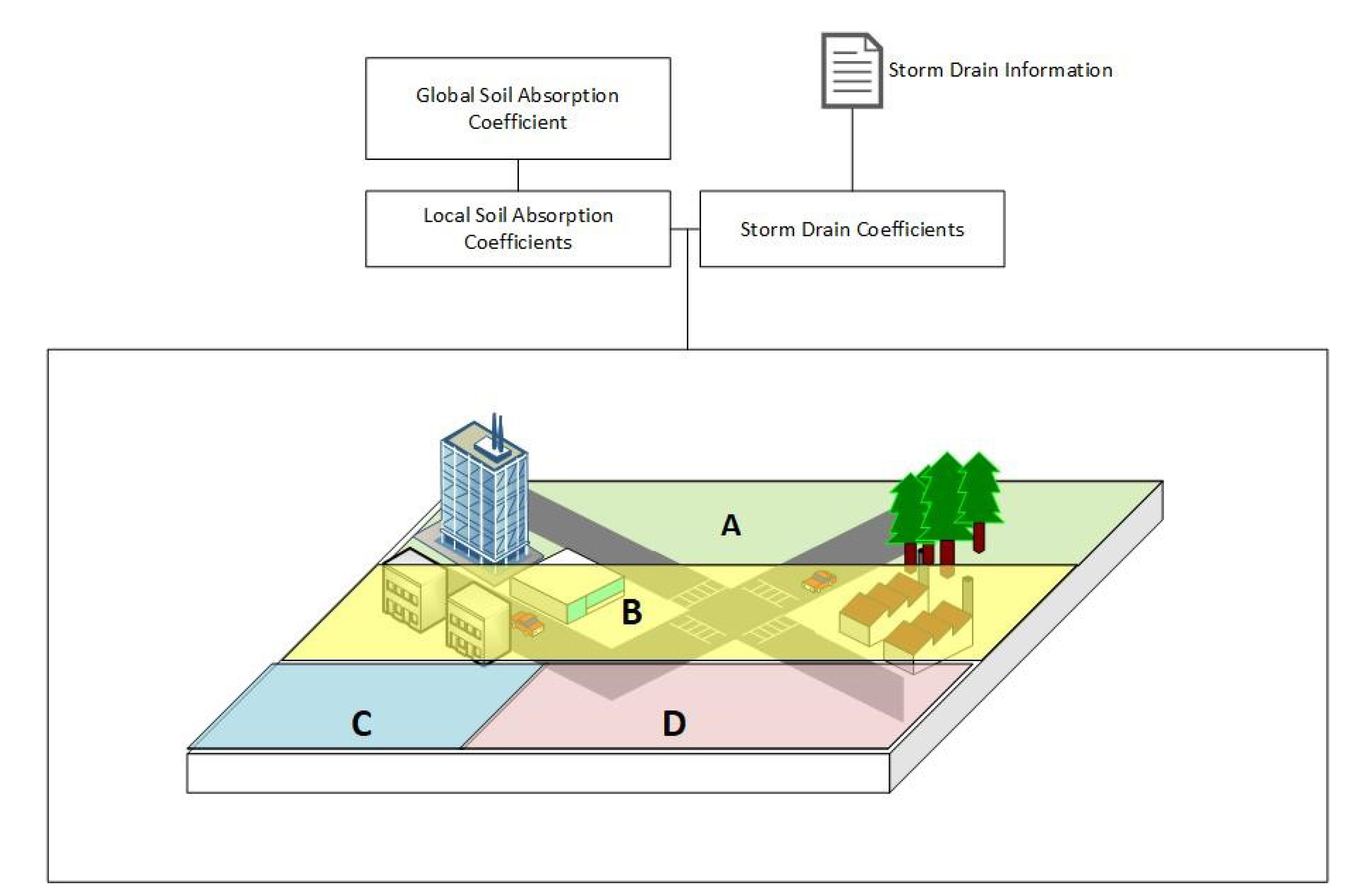
As particle-based simulations focus on particles’ interactions with the surrounding environment, too much interaction may cause slow performance, simulation instability, and consequently, visual anomalies. To prevent this, our work proposes global and local soil absorption coefficients for the study area, and particle removal is handled according to these coefficients. Furthermore, storm drain information, if available, is incorporated into this model, and can be visualized in any resolution that the study area requires. Figure 4 shows an overview of the soil absorption mechanics and how it places absorption coefficients across the virtual environment.
In this figure, reading the information from storm drain data and utilizing other global and local soil absorption coefficients, regions A, B, C and D are defined. These regions have different absorption values and thus water particles are removed at different rates. It is possible to provide a very high resolution by providing unique locations of every single side inlet, sacrificing performance in the process. Nevertheless, for real-time simulation, it might not be the most appropriate solution. An adaptive approach benefits both the demand of performance and detail in description. Consequently, our work provides an adaptive approach in which grid sizes may be altered on demand to provide both performance and detail.
The storm drain document is a vital part of this implementation, as it contains detailed representation of the environment and where the inlets are placed. This document provides longitudes, latitudes, and flow line elevation information for the absorption computation to run appropriately. As such information might be incomplete or unavailable, resolution can be decreased to represent an overall absorption for given areas instead of focusing on individual inlets. This is done through utilization of an adaptive grid [43] as discussed earlier, by using a quadtree to divide the study area into grids. By predefining a proper level of depth as required for the study, absorption is computed through averaging the inlets’ properties in generated cells. This behavior is then visualized in 3D, through particle removal per simulation second, as part of the flood simulation framework. Overall, this process is efficient because predefined cells contain a fixed number of inlets and therefore computations of absorption coefficients are done prior to fluid simulation.
2.4. Cloud and Rainfall Mechanics
Rainfall must be described in a meaningful way such that its inherent behavior can be properly represented in 2D and 3D simulations. This behavior mostly comes from the observations that we can find for the given study area. Nevertheless, it might also be preferable to conduct experiments instead of following and engineering the existing data for the purpose of visualization. This module utilizes rainfall intensity data to generate instances of cloud objects over the study area to represent the rainfall in the 3D environment. Furthermore, custom clouds can be defined and placed around the map with differing rainfall intensities, sizes, and speeds. Hence, cloud and rainfall mechanics offers full customization of how the particles are added to the simulated environment. Together with soil absorption mechanics, they define the addition and removal of particles from the environment and thus are vital components of the simulation for the purpose of efficiency.
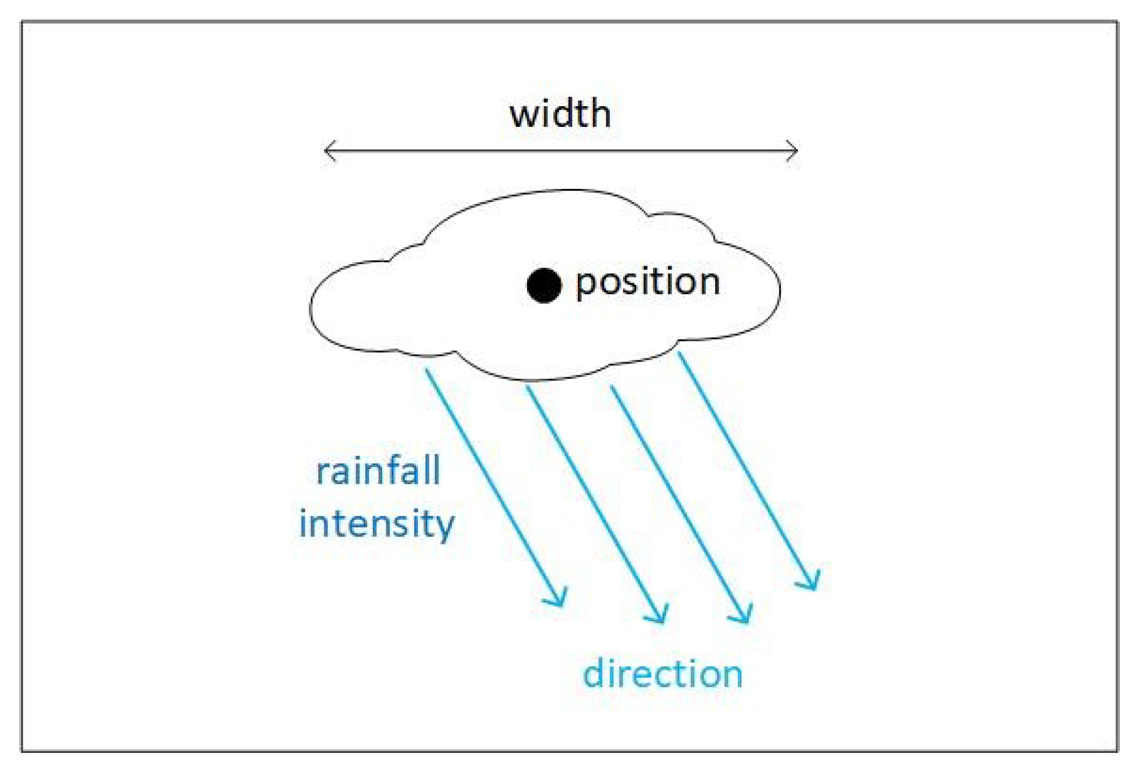
Cloud objects are formed using several parameters to describe the rainfall. These objects are read from a cloud configuration file, which holds references to the clouds with their identifiers, position, rainfall, and rainfall intensity. At this point, it is possible to activate the clouds to make the rainfall occur, but this is normally done dynamically using cloud animation objects to dictate cloud behavior in the simulation. A vector keeps track of the cloud references and the objects get processed at every time step. There is no limit to the maximum number of clouds that can be generated in the study area. Nonetheless, there is a hard particle number limit for real-time simulation purposes, which might stop clouds producing additional rainfall. Figure 5 shows a representation of a cloud object.
Cloud position is derived from the geographic coordinates found in the cloud configuration file. In most cases, this information is implemented manually and therefore initial evaluation of the rainfall data may be required. Upon checking available rainfall data for the city, practitioners can divide the city into several subsections, define clouds, or areas where rainfall occurs, and then input the expected rainfall amount for the given area.
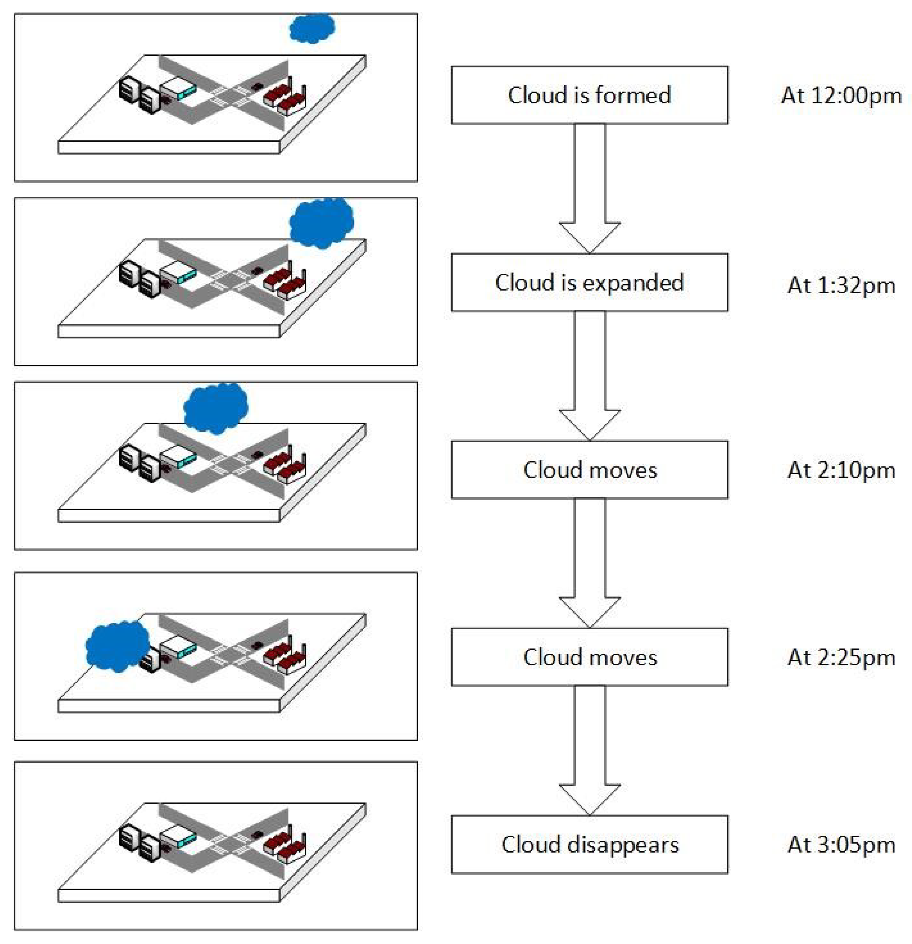
Cloud animation objects are extensions of cloud objects. Each cloud object comes with an additional cloud animation object associated with itself. These cloud animation objects carry keyframe information to specify important changes over time such as cloud movement and rainfall intensity changes. Moreover, an active cloud can be deactivated after a certain amount of time. The keyframes contain start and end timestamps to define an animation. When the cloud animation objects are loaded into the scene, the vectors containing these objects are passed to the visualization engine. At this stage, the visualization engine restructures the data and processes keyframe information as the time passes. Multiple timers are utilized to account for the CPU time, simulation time, and animation times and therefore it is possible to slow down or speed up these animations.
Available animations provided for cloud animation objects are the creation, translation, and deletion of clouds; altering rainfall intensity; changing the direction of rainfall; and altering the width of clouds. Some of these actions (e.g., altering rainfall intensity) can be initialized as gradually changing over time. If gradual change is not set up, then an immediate change occurs at a given timestamp. The timestamp feature utilizes 24-h notation to determine the time of events written in a cloud animation configuration file.
If rainfall data can be acquired, then cloud animation objects can be helpful in designing a real-world scenario and evaluating the results for calibrating the local dynamics of the system. Utilizing the acquired timestamps, the cloud configuration files can carry real-world precipitation information and visualize the event in the system through appropriate calibration of the local environment. Figure 6 shows a representation of how cloud animation data files work and how they help the simulation engine to visualize cloud information over time.
An advantage of using the cloud animation objects is that the simulation environment becomes quite extensible and allows users to manipulate information in real time. Furthermore, such conditions can be recorded and logged into a data file for rebuilding the same environment. Although the randomization in the wind factor, rainfall splatter, and GPU processing would alter the visualization to some extent, it would be possible to recreate similar conditions and evaluate the environment parameters. Another advantage is provided through the provision of dynamic parameters for the cloud. Not only the position and rainfall intensity, but any other parameter can be given values and be animated over time. This allows for interpolation of the unknown data, as the user can define a command like “increase the intensity by 5 mm over an hour”. Therefore, rather than utilizing abrupt changes of environmental parameters, a smooth transition can occur, which would potentially help practitioners incorporate their data into the simulation environment.
2.5. Workflow
The simulation engine is prepared through reading scene descriptions. These data files contain information about the environment, such as terrain and object placement, simulation parameters, and several other pieces of environmental information. Initially the environment is loaded as the terrain for the scene. Terrain objects can be a singular unified entity or can consist of hundreds of separate pieces. The advantage of utilizing a unified body is that the simulation runs more efficiently. As the object does not contain subparts to be evaluated further once particle interaction occurs, the computation is handled in a straightforward fashion. The disadvantage is obviously the lack of feature differentiation, and therefore it might be detrimental if local friction coefficients are to be utilized. Conversely, the advantage of utilizing multi-part terrain is the inclusion of a local friction model with the cost of additional computation per feature placed in the terrain. This might come with a substantial loss of performance, especially for larger areas, considering that one of our main focuses is to provide an efficient flood simulation framework.
After the terrain and some simulation parameters (e.g., maximum number of particles) are initialized as defined by the user, environmental configuration files are read. By reading these files and initializing data structures to be utilized in the computation, the environment is organized for the simulation. After this, a digital elevation model (DEM) is generated from the terrain to be used for depth computation once the simulation begins. With the creation and storage of the height map, the simulation starts executing and producing results as requested.
Initially, the depth map and related storage, such as a regular grid and a quadtree with provided maximum depth, are created to support 2D tracking of depth. With this approach, the simulation can be visualized in a mini map placed at the bottom-right of the simulation environment alongside 3D information in the main simulation screen. This mini map provides depth information as the water traverses the environment. By providing a 2D view of the environment while getting the benefits of 3D simulation, as underlined in [22], we provide better clarity of the depth information of flooding across the study area.
Upon initialization of the 2D mapping module [43], the environment and relevant objects are updated per frame. The clouds are set to emit the water particles with given rainfall intensity and direction. Upon creation of these particles, the buffers are utilized to track different aspects of the particles (positions, velocities, densities, and several other parameters). These parameters are vital for the position-based fluids simulation environment to work properly.
Every simulation second, the engine sends an “absorb” message to the soil absorption module, which is responsible for checking environmental soil absorption coefficients and processing the requests coming from the simulation engine. If the module recognizes the particles touching the soil, it utilizes the absorption rates defined for the sections of the simulation environment to remove these particles from the environment. The cloud animation data file is read during scene initialization, and therefore the simulation engine has the knowledge of all future events at this stage. The engine considers the current simulation time and examines the timestamp information embedded into cloud animation objects to estimate if new events will occur at the current timestamp. Furthermore, if cloud parameters are currently being animated, the simulation engine calculates the parametric changes that will occur in the next frame and passes this information to the drawing component. In the next frame, the drawing component flushes the updated parameters.
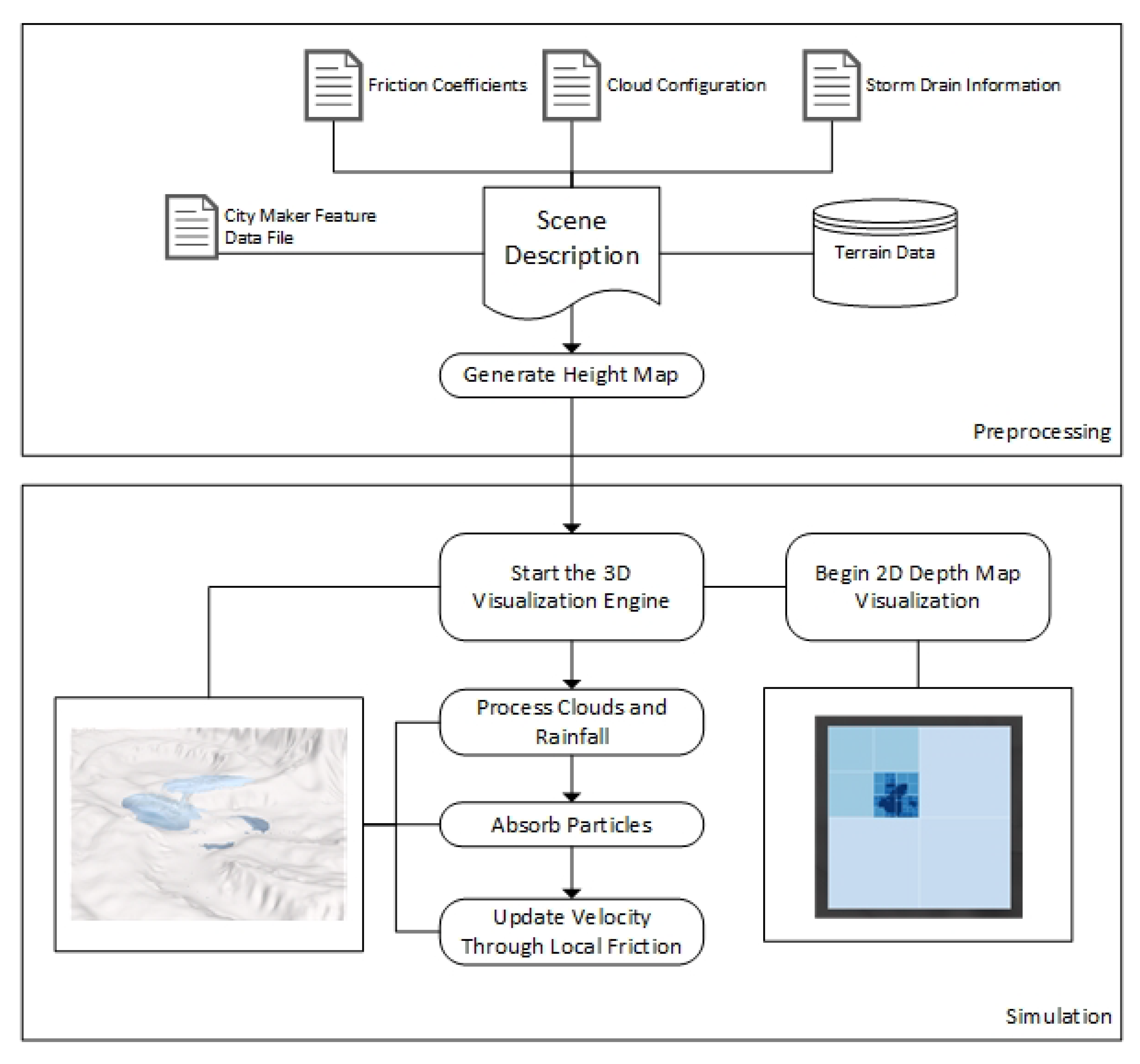
These operations continue until the simulation is halted per user request. For the purpose of this work, we considered refreshing the parameters and processing the depth information every second, setting the required frame rate to 60 frames per second. If efficiency is not a concern, this parameter could possibly be initialized using milliseconds instead of seconds. A typical workflow in FloodSim is represented in Figure 7.
3. Results and Discussion
In this section we show how the system can be utilized in a variety of scenarios to show the interaction of water with the environment. Initially, FloodSim mechanics are demonstrated through utilizing hypothetical environments and the digital model of Corpus Christi, TX, USA. We also provide a case study that simulates a historical flood to show the visual fidelity of FloodSim.
3.1. Utility of Various Mechanics and Performance
Upon initialization of FloodSim, several tests were performed to demonstrate the capabilities of different mechanics utilized in the simulation. As discussed in Section 2, there are three major engine components built into FloodSim: global and local friction model, soil absorption mechanics, and cloud/rainfall mechanics. These mechanics are intended to work together to define simulation mechanics that dictate how the water behaves in the environment. For a hypothetical environment, several random parameters are defined. For Corpus Christi, randomized precipitation data were utilized alongside the storm sewer data file to define absorption areas appropriately.
FloodSim uses parameters to define the friction between water particles and the environment. Figure 8a shows an example terrain without the use of the local friction coefficients, thus utilizing only the default parameters, which only account for default surface friction and particle friction coefficients. Figure 8b shows the same environment with the inclusion of local friction coefficients to represent high vegetation. To simplify the demonstration, the environment is defined as an “area with high vegetation” for its entirety. Through realization of the environmental parameters, velocity is decreased according to the Manning formula. Consequently, this extra friction stops the water from spreading out as quickly and thus contains the water.
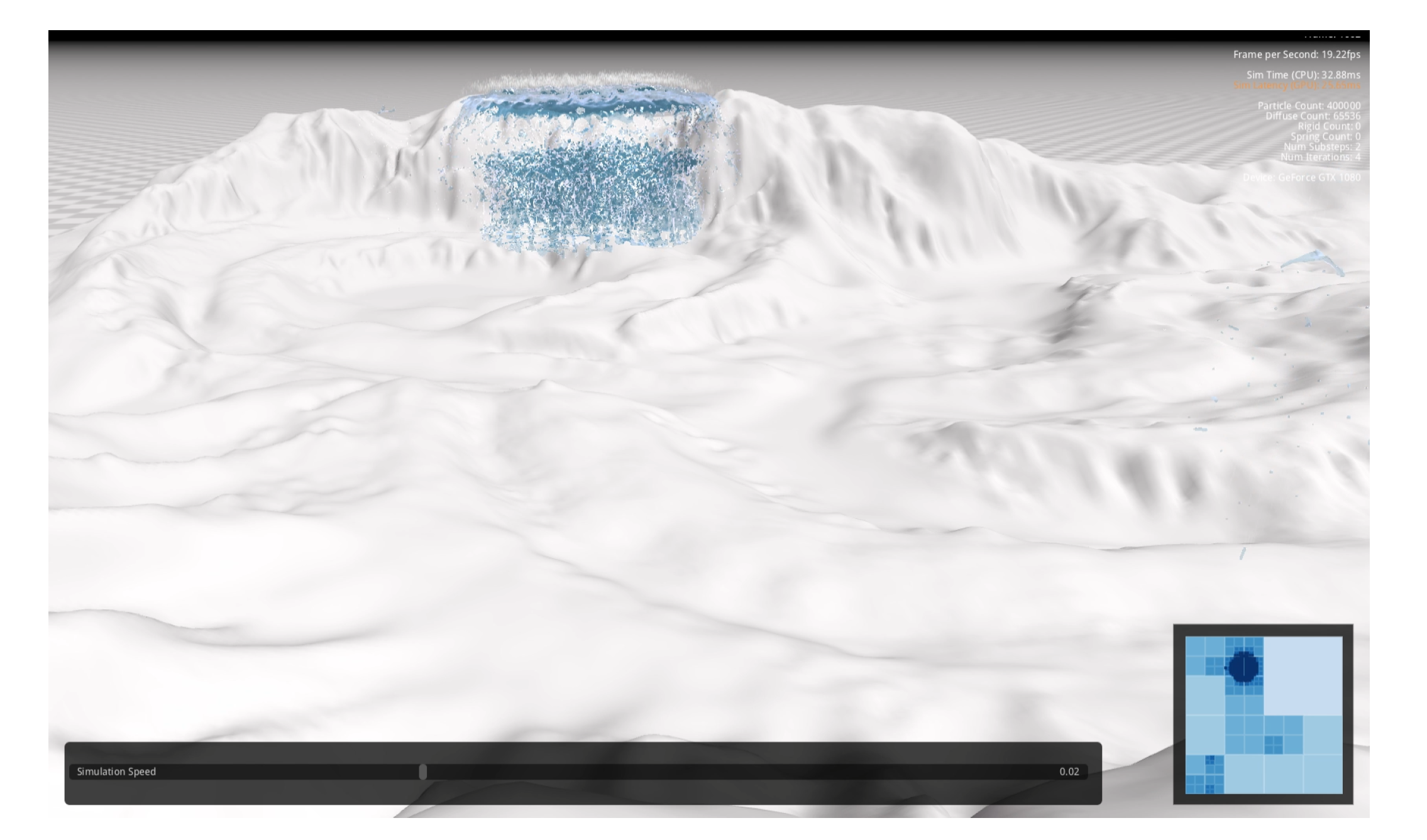
Rainfall and cloud mechanics form the basis of how particles are created for the environment, and consequently they are vital for the system. The cloud mechanics were tested by creating a cloud with such a large width that it could drop a high amount of particles into the environment. This large cluster is shown in Figure 9. In this test, an extreme rainfall amount corresponding to 400K particles in FloodSim were dropped on a selected location through a cloud. Such large areas can be selected with more reasonable amounts of precipitation for interpolation of rainfall across an area. This test used an extreme case just to demonstrate the capabilities of clouds.
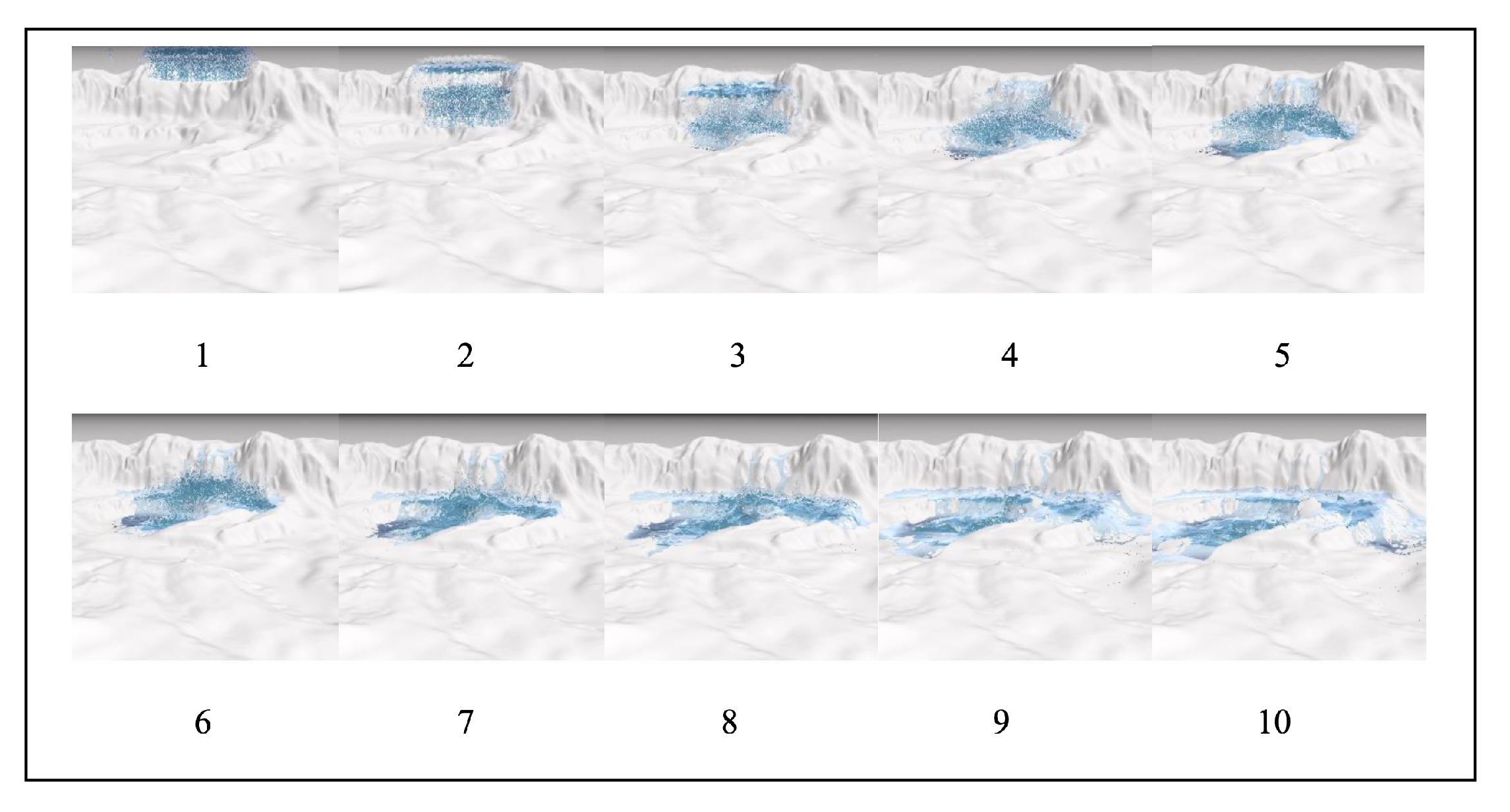
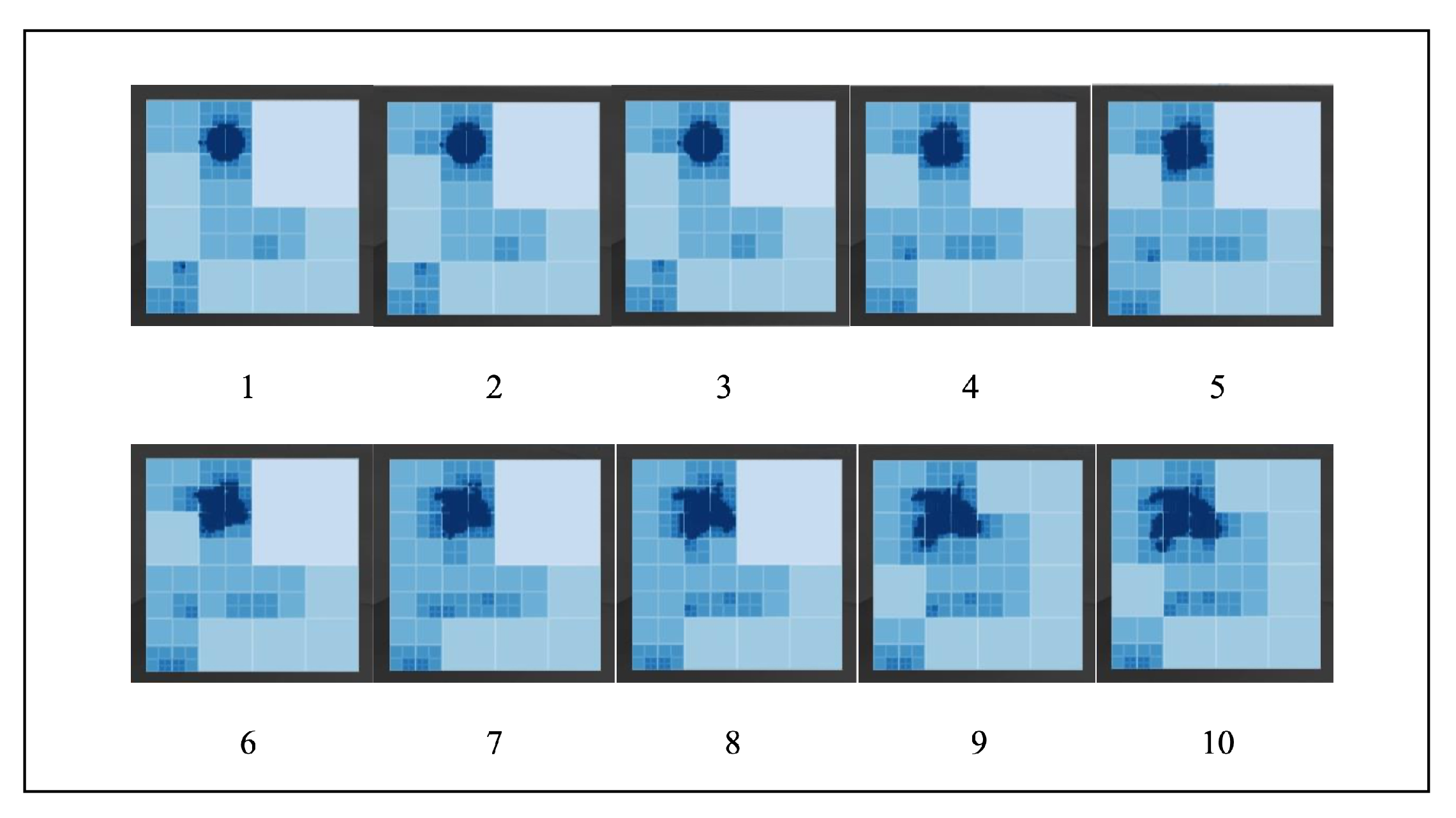
Figure 10 and Figure 11 show frames from the flood simulation over time in 3D and a 2D depth map. The depth map helps visualize the flood spread clearly while the 3D view provides an additional perspective of depth to visualize the flooding. Both views are useful in presenting the environment and how flooding progresses over time, and using both increases understanding of how the waters spread.
Although it is apparent that the mechanics implemented for FloodSim are all required to represent the fluid dynamics properly, the system could not proceed with the simulation without absorption mechanics. As the particle removal is a vital factor for efficiency purposes, leaving this mechanic out is not an option to run the simulation for longer times. With the data of storm drainage information acquired from the city of Corpus Christi, City Maker [42] was utilized to parse the information into environmental data. The absorption tests were performed upon parsing this data.
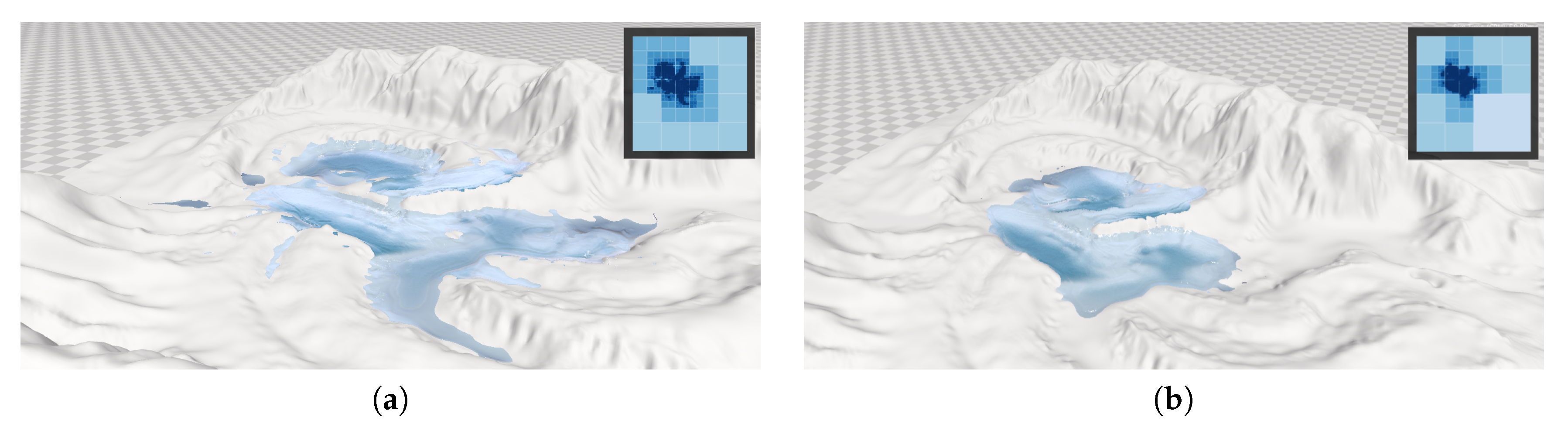
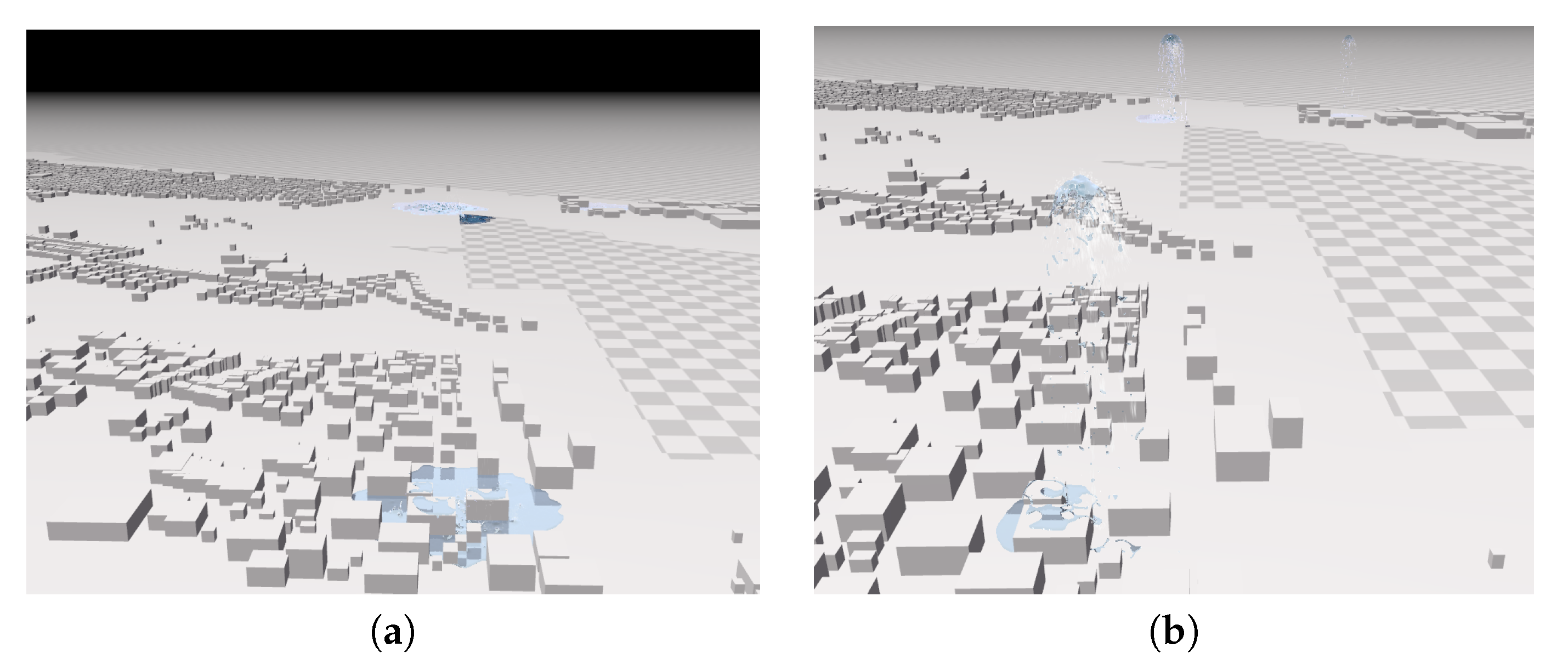
Figure 12a,b show the differences in flooding achieved using our absorption mechanism. Utilizing light rainfall in three different spots on the map, particle clustering was tracked. As the rain is generated by rainfall and cloud mechanics, the particles are dropped into the environment using gravity as the force. Using the coefficients derived from the previous stage, the scene with the absorption considers the particles generated by rainfall and by applying a rate of absorption, removes these particles as they touch the surface. If there is no absorption coefficient set up, as in the case of Figure 12a, then the particles are never removed—water simply flows over the surface until the simulation is terminated. With soil absorption, the inlets and the passive absorption coefficient, the result is more fitting for a light rain scenario, as can be seen in Figure 12b. This helps with efficiency through particle removal and visual fidelity as it accounts for evaporation and absorption.
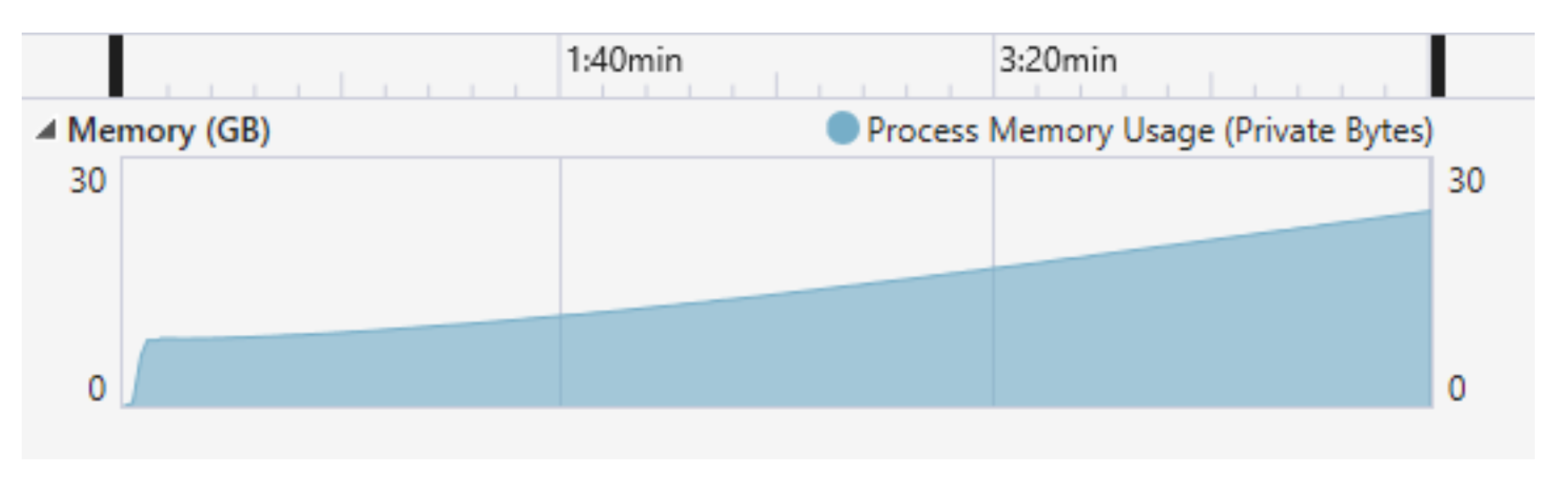
To run these simulations, an Alienware Aurora R6 with Intel i7-7700K processor, NVIDIA GeForce 1080 display adapter, and 32 GB of physical RAM was utilized. First, the framework was tested for memory usage, disabling soil absorption and particle removal. Figure 13 shows that with constant particle generation for 5 min, 3.5 million particles were generated and 23.8 GB of RAM was used up. As memory would be required to continue the processes within the solver and compute interaction between particles, it would not be feasible to work with such a setup. Therefore, scalability is an important concern for the simulation of larger areas. Fewer particles means less detail in the description of flooding, and therefore errors should be expected. Such errors must be accounted for through the provision of precise details about the study area and utilization of more capable CPUs and GPUs.
Next, several hypothetical environments with the same size were used to test the performance of the engine. These tests were performed with a focus on particle interaction, and thus particle counts remained the same in each scenario. According to Table 1 it is clear that an increase in the number of particles was detrimental to the performance. Buildings cause more interaction between particles and surfaces, and therefore they hinder performance. Considering the terrain as a static mesh, as opposed to separate individual components, alleviated performance issues. For the description of larger environments, additional data structures can be utilized to improve performance.
3.2. River Flooding Case Study
We used the Bewdley flood of 2000 as a case study for our system. We chose to simulate this particular flood as there is historical data available and there are results from another work [48] using this flood, allowing us to compare their results to those obtained from our system. Bewdley, Worcestershire, United Kingdom, was one of the towns that got the effect of flooding which occurred in Fall 2000 along the Severn Valley. The town was flooded three times within six weeks, and therefore measures needed to be taken to improve flood defenses, emergency management efforts, and flood warning systems.
For flooding visualization, only a section of Bewdley was selected and Shuttle Radar Topography Mission (SRTM) with 30 m resolution was utilized for providing the elevation information. As it is a river flooding scenario, a certain threshold for maintaining the depth of the environment was arranged so that the riverbed did not experience draught, unlike the rest of the environment. Upon calibrating the height values to represent flooding and arranging particle sizes for the simulation and constraining the river water, the environment was placed in the scene for further arrangements.
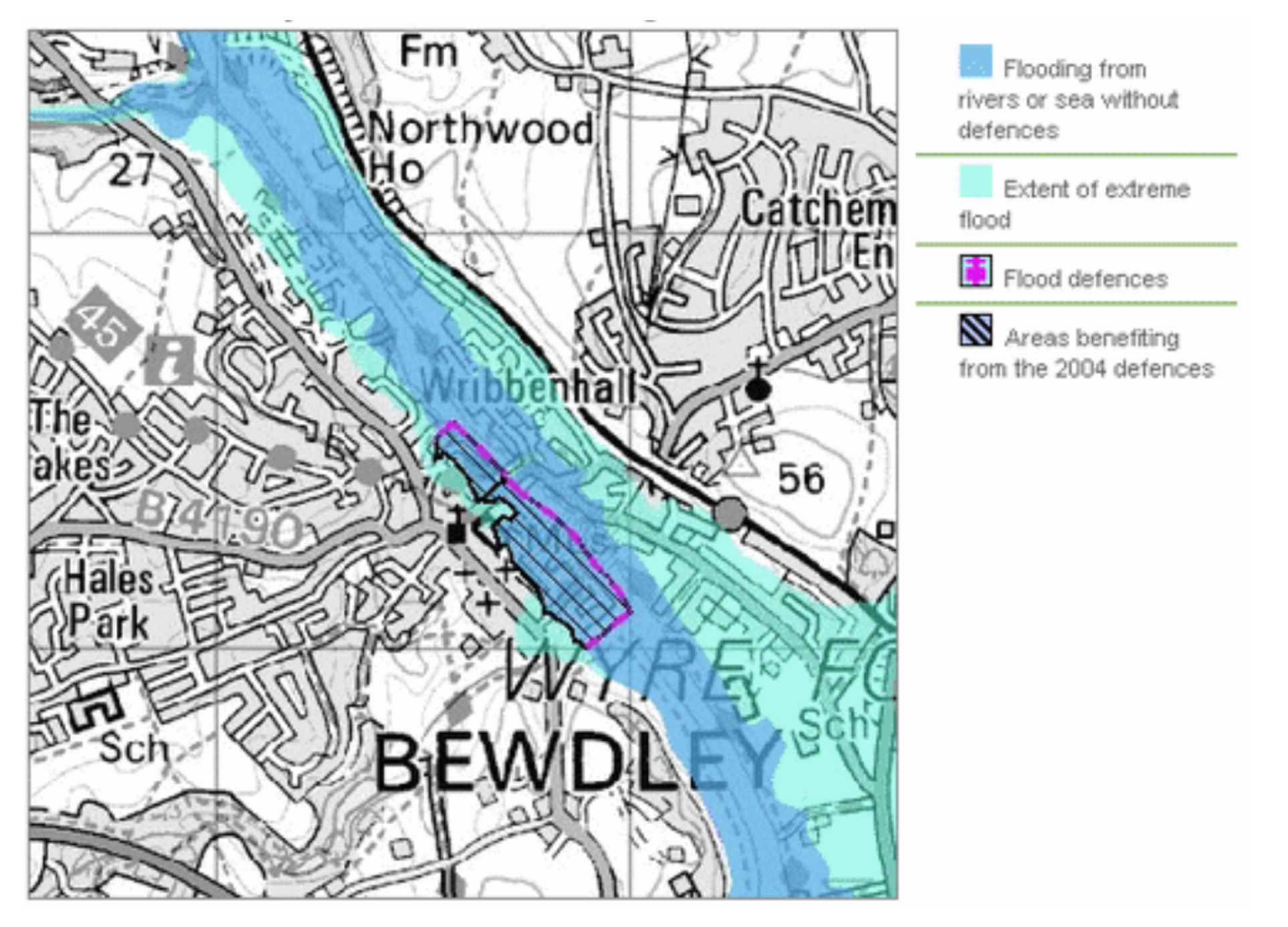
For testing visual realism, the Bewdley flooding case study was acquired and data is utilized to generate similar conditions. With the choices of simulation parameters, around 1 million particles were required to get the flood to similar levels as in the actual flooding. Furthermore, 300,000 particles were required to simply fill the riverbed, with depths acquired from bathymetric data, for proper representation of the river. Upon stabilization of the particles, rainfall was provided through clouds that were interpolated over the river. Fourteen clouds distributed at equal distances above the riverbed produced sufficient rainfall for the event to be recreated. Figure 14 shows the map found for Bewdley showing the river flooding event, possible flood extent, and flood defenses. This map was acquired to show a comparison with the expected flooding extent of the area and the results produced by FloodSim.
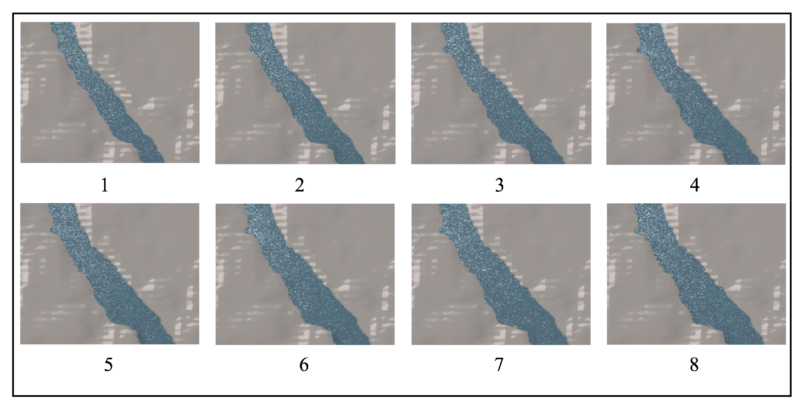
Frames from an animation of the river flooding are provided in Figure 15. Flooding was captured around every 100,000 particles of increase in water amount and lasted a total of 220 s. Once the simulation reached approximately 1 million particles, the amount of water required to demonstrate the flooding was placed into the riverbed. Additional time was reserved for waiting for the simulation to reach a stable state. Upon visual investigation of Figure 14 and the result generated by FloodSim, it can be seen that the flooding area was visualized similarly. Nevertheless, some parts of the flooding were not visualized accurately. This is partly due to flood defenses, which our method does not account for, and due to the resolution of SRTM, which FloodSim works with. Improving the DEM model and providing a more detailed river bathymetry would improve results. Nevertheless, performance is still a concern if the current configuration of CPU and GPU are to be utilized.
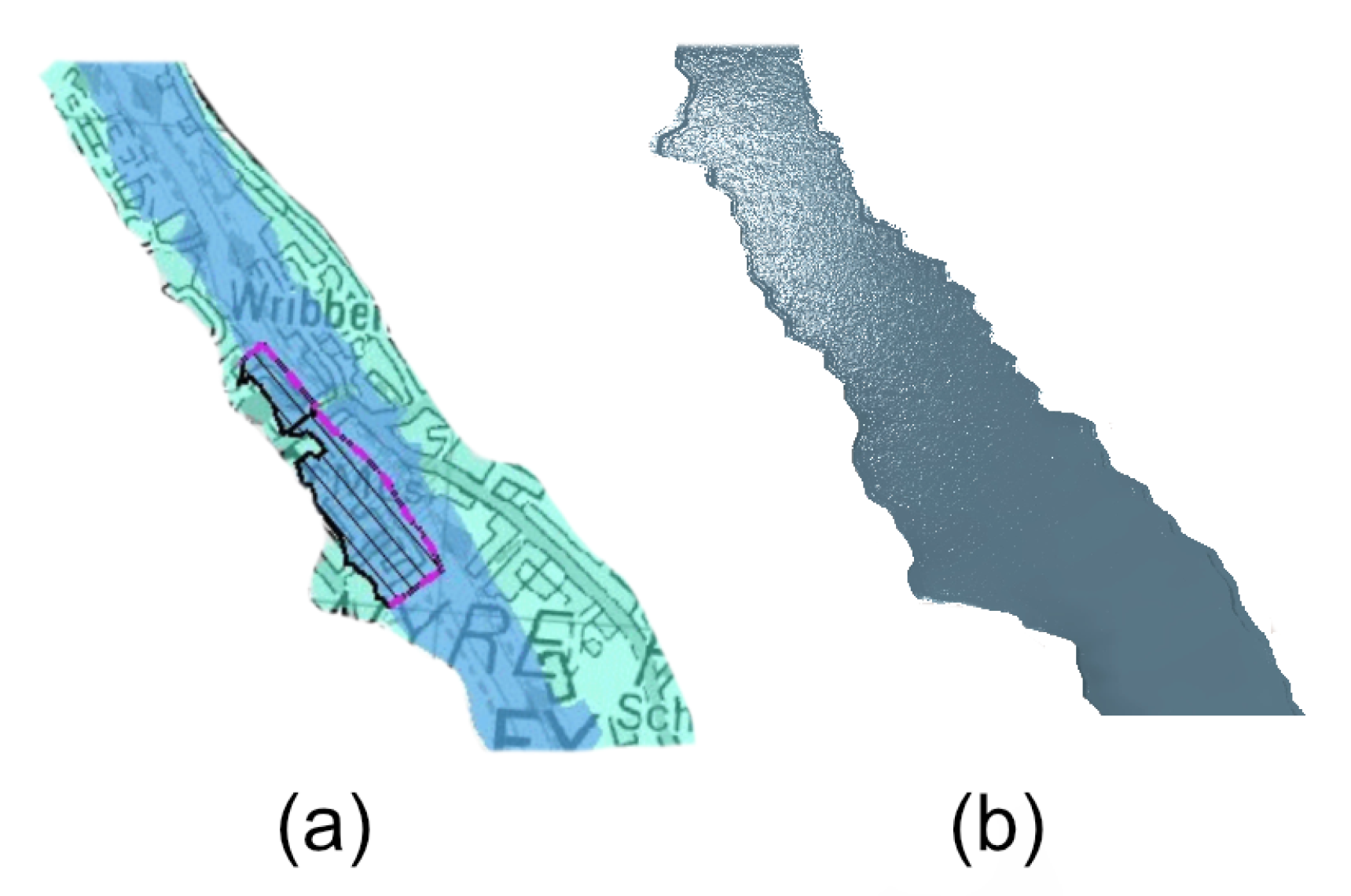
Figure 16 shows an isolated comparison of river sections upon flooding. Visually, we can reiterate that FloodSim performed well visually to represent the extent of flooding. Further refinements can be made to improve the visual fidelity. However, this shows the feasibility of the use of position-based fluids (PBF) for a flooding scenario, which is not commonly used in the industry. An advantage of FloodSim is that it utilizes a Lagrangian description of fluid flow, which allows the user to investigate individual particles while still performing fast enough to view the occurrence as it progresses. Consequently, bigger scenarios and larger extents may be worth investigating with FloodSim to gain a better insight into particle behavior.
For the output, the same sections of the river flooding from the bridge at Load St. to Kidderminster Rd. were extracted and flooding extents were calculated. These areas were then compared side-by-side to clarify any potential differences. Based on the geographic extent of the selected area, the section showed an approximate 12,224 m2 of inundation according to Figure 16a while FloodSim determined 11,395 m2 of inundation as shown in Figure 16b. The difference computed was around 7%. This shows the feasibility of position-based fluids in the description of surface flow and determination of flooding extent. Considering that SRTM data with a resolution of 30 m were used to generate the terrain, it is realistic enough to be considered as a basis for developing a position-based flood simulator. Further experiments could be conducted to calibrate the model further and comparisons could be made with more recent river flooding models to compare visual fidelity.
4. Conclusions and Future Work
The framework described in this work provides a workflow to demonstrate the usability of position-based fluids to simulate and visualize flooding events. As position-based fluids are more suited for real-time simulations than some traditional SPH models, the provision of this framework allows for real-time interaction through efficient particle representation. The addition of friction model, cloud and rainfall mechanics, along with the soil absorption provides dynamic representation of the study area. As the results show, by using environmental data through SRTM elevation with 30 m resolution, river flooding simulations can be performed with a realistic representation of the study area. As the purpose of the framework is to have an efficient position-based fluids framework for visualizing and simulating flooding, the results are appropriate.
FloodSim was designed with parameters such as rainfall, soil absorption, and water drainage to simulate a wide variety of flooding scenarios. This work presents a new flood visualization and simulation framework with position-based fluids by providing the benefits of position-based dynamics [40] to contain particles and prevent usual neighborhood problems [36] that occur in SPH [38], contributing efficiency. To our knowledge, the position-based fluids approach has not been investigated in depth in the flood modeling community. Consequently, the provision of this framework yields an alternative approach for the visualization and simulation of flooding phenomena. Such a framework, with further calibration to incorporate a quantitative flood model, can be utilized to test different scenarios regarding flooding to visualize a city’s or an area’s resilience against flooding events. Considering that empirical and many hydrological models provide a grid-based approach to describe the fluid flow, our model utilizes a particle-based Lagrangian approach which has certain advantages over such models to provide more insight about the local fluid particle behavior. Although it can be underlined that Eulerian models visualize continuum properly, Lagrangian models with more advanced GPUs help experiment with the study area utilizing particle interaction. Consequently, this work can be used alongside other frameworks to provide a different perspective regarding the study area since it allows refinements in the hands of practitioners to describe the local dynamics of an environment more precisely.
As underlined earlier, many of the environmental parameters are loaded through the component reader. These parameters are not altered after the initial processing. Simulating a fully dynamic environment with shifting wind direction over time, intensifying the rain, and considering soil erosion and soil absorption could yield interesting results. Such scenarios should be implemented and experimented with in the future to provide a more precise simulation framework for utilization in real-world scenarios such as risk assessment and emergency management. Upon the description of a more detailed flood model for specialized purposes, recent flood models in the industry could be compared with FloodSim to recognize hte advantages and disadvantages of utilizing a position-based approach.
Further investigation must be done to clarify scalability issues of the flood simulation framework. Although the data can be parsed and large city models can be reconstructed with the current approach, SRTM data provides low-resolution elevation information that prevents us from proceeding with a higher-resolution simulation. City-wide or region-wide simulations will be incorporated in future work with the utility of higher-resolution elevation data.
Author Contributions
Conceptualization, I. Alihan Hadimlioglu and Scott A. King; methodology, validation, writing—original draft preparation, I. Alihan Hadimlioglu; writing—review and editing, Scott A. King and Michael J. Starek; visualization, I. Alihan Hadimlioglu. All authors have read and agreed to the published version of the manuscript.
Funding
This research received no external funding.
Conflicts of Interest
The authors declare no conflicts of interest.
References
- Bertilsson, L.; Wiklund, K.; Tebaldi, I.; Rezende, O.M.; Veról, A.P.; Miguez, M.G. Urban flood resilience—A multi-criteria index to integrate flood resilience into urban planning. J. Hydrol. 2019, 573, 970–982. [Google Scholar] [CrossRef]
- Khosravi, K.; Pham, B.T.; Chapi, K.; Shirzadi, A.; Shahabi, H.; Revhaug, I.; Prakash, I.; Bui, D.T. A comparative assessment of decision trees algorithms for flash flood susceptibility modeling at Haraz watershed, northern Iran. Sci. Total Environ. 2018, 627, 744–755. [Google Scholar] [CrossRef] [PubMed]
- Lyu, H.; Sun, W.; Shen, S.; Arulrajah, A. Flood risk assessment in metro systems of mega-cities using a GIS-based modeling approach. Sci. Total Environ. 2018, 626, 1012–1025. [Google Scholar] [CrossRef] [PubMed]
- Machado, M.J.; Botero, B.A.; López, J.; Francés, F.; Díez-Herrero, A.; Benito, G. Flood frequency analysis of historical flood data under stationary and non-stationary modelling. Hydrol. Earth Syst. Sci. 2015, 19, 2561–2576. [Google Scholar] [CrossRef] [Green Version]
- Brázdil, R.; Kundzewicz, Z.W.; Benito, G. Historical hydrology for studying flood risk in Europe. Hydrol. Sci. J. 2006, 51, 739–764. [Google Scholar] [CrossRef]
- Teng, J.; Jakeman, A.; Vaze, J.; Croke, B.; Dutta, D.; Kim, S. Flood inundation modelling: A review of methods, recent advances and uncertainty analysis. Environ. Model. Softw. 2017, 90, 201–216. [Google Scholar] [CrossRef]
- Didier, D.; Bernatchez, P.; Boucher-Brossard, G.; Lambert, A.; Fraser, C.; Barnett, R.L.; Van-Wierts, S. Coastal flood assessment based on field debris measurements and wave runup empirical model. J. Mar. Sci. Eng. 2015, 3, 560–590. [Google Scholar] [CrossRef]
- Leandro, J.; Chen, A.S.; Djordjević, S.; Savić, D.A. Comparison of 1D/1D and 1D/2D coupled (sewer/surface) hydraulic models for urban flood simulation. J. Hydraul. Eng. 2009, 135, 495–504. [Google Scholar] [CrossRef]
- Liao, Z.; Xu, Z.; Wang, D.; Lu, S.; Hannam, P.M. River environmental decision support system development for Suzhou Creek in Shanghai. J. Environ. Manag. 2011, 92, 2211–2221. [Google Scholar] [CrossRef]
- Wang, Y.; Liu, R.; Guo, L.; Tian, J.; Zhang, X.; Ding, L.; Wang, C.; Shang, Y. Forecasting and Providing Warnings of Flash Floods for Ungauged Mountainous Areas Based on a Distributed Hydrological Model. Water 2017, 9, 776. [Google Scholar] [CrossRef] [Green Version]
- Gabellani, S.; Silvestro, F.; Rudari, R.; Boni, G. General calibration methodology for a combined Horton-SCS infiltration scheme in flash flood modeling. Nat. Hazards Earth Syst. Sci. 2008, 8, 1317–1327. [Google Scholar] [CrossRef]
- Chen, Y.; Li, J.; Huang, S.; Dong, Y. Study of Beijiang catchment flash-flood forecasting model. Proc. Int. Assoc. Hydrol. Sci. 2015, 368, 150–155. [Google Scholar] [CrossRef] [Green Version]
- Roux, H.; Labat, D.; Garambois, P.A.; Maubourguet, M.M.; Chorda, J.; Dartus, D. A physically-based parsimonious hydrological model for flash floods in Mediterranean catchments. Nat. Hazards Earth Syst. Sci. 2011, 11, 2567–2582. [Google Scholar] [CrossRef] [Green Version]
- Wester, S.J.; Grimson, R.; Minotti, P.G.; Booij, M.J.; Brugnach, M. Hydrodynamic modelling of a tidal delta wetland using an enhanced quasi-2D model. J. Hydrol. 2018, 559, 315–326. [Google Scholar] [CrossRef]
- Leskens, J.G.; Kehl, C.; Tutenel, T.; Kol, T.; de Haan, G.; Stelling, G.; Eisemann, E. An interactive simulation and visualization tool for flood analysis usable for practitioners. Mitig. Adapt. Strateg. Glob. Chang. 2017, 22, 307–324. [Google Scholar] [CrossRef] [Green Version]
- Liu, X.; Zhong, D.; Tong, D.; Zhou, Z.; Ao, X.; Li, W. Dynamic visualisation of storm surge flood routing based on three-dimensional numerical simulation. J. Flood Risk Manag. 2018, 11, 729–749. [Google Scholar] [CrossRef]
- Liu, J.; Gong, J.; Liang, J.; Li, Y.; Kang, L.; Song, L.; Shi, S. A quantitative method for storm surge vulnerability assessment—A case study of Weihai city. Int. J. Digit. Earth 2017, 10, 539–559. [Google Scholar] [CrossRef]
- Luettich, R.A., Jr.; Westerink, J.J.; Scheffner, N.W. ADCIRC: An Advanced Three-Dimensional Circulation Model for Shelves, Coasts, and Estuaries. Report 1. Theory and Methodology of ADCIRC-2DDI and ADCIRC-3DL; Dredging Research Program Tech. Rep. DRP-92-6; U.S. Army Engineers Waterways Experiment Station: Vicksburg, MS, USA, 1992; p. 143. [Google Scholar]
- Bender, J.; Finkenzeller, D.; Oel, P. HW3D: A tool for interactive real-time 3D visualization in GIS supported flood modelling. In Proceedings of the 17th International Conference on Computer Animation and Social Agents, Geneva, Switzerland, 7–9 July 2004; pp. 305–314. [Google Scholar]
- Toros, H.; Kahraman, A.; Tilev, C.; Geertsema, G.; Cats, G. Simulating Heavy Precipitation with HARMONIE, HIRLAM and WRF-ARW: A Flash Flood Case Study in Istanbul, Turkey. Eur. J. Sci. Technol. 2018, 13, 1–12. [Google Scholar] [CrossRef]
- Bao, Y.; Huang, Y.; Liu, G.R.; Zeng, W. SPH Simulation of High-Volume Rapid Landslides Triggered by Earthquakes Based on a Unified Constitutive Model. Part II: Solid-Liquid-Like Phase Transition and Flow-Like Landslides. Int. J. Comput. Methods 2018. [Google Scholar] [CrossRef]
- Van Ackere, S.; Glas, H.; Beullens, J.; Deruyter, G.; De Wulf, A.; De Maeyer, P. Development of a 3D dynamic flood WebGIS visualisation tool. Int. J. Saf. Secur. Eng. 2016, 6, 560–569. [Google Scholar] [CrossRef] [Green Version]
- Zhang, S.; Xia, Z.; Wang, T. A real-time interactive simulation framework for watershed decision making using numerical models and virtual environment. J. Hydrol. 2013, 493, 95–104. [Google Scholar] [CrossRef]
- Macchione, F.; Costabile, P.; Costanzo, C.; De Santis, R. Moving to 3-D flood hazard maps for enhancing risk communication. Environ. Model. Softw. 2019, 111, 510–522. [Google Scholar] [CrossRef]
- Brunner, G.W. HEC-RAS River Analysis System. Hydraulic Reference Manual. Version 5.0. 2016. Available online: https://www.hec.usace.army.mil/software/hec-ras/documentation/HEC-RAS%205.0%20Reference%20Manual.pdf (accessed on 20 October 2019).
- Yang, J.; Townsend, R.D.; Daneshfar, B. IApplying the HEC-RAS model and GIS techniques in river network floodplain delineation. Can. J. Civil Eng. 2006, 33, 19–28. [Google Scholar] [CrossRef]
- Thol, T.; Kim, L.; Ly, S.; Heng, S.; Sreykeo, S. Application of HEC-RAS for a flood study of a river reach in Cambodia. In Proceedings of the 4th International Young Researchers’ Workshop on River Basin Environment and Management, Ho Chi Minh City, Vietnam, 12–13 November 2016. [Google Scholar]
- Yakti, B.P.; Adityawan, M.B.; Farid, M.; Suryadi, Y.; Nugroho, J.; Hadihardaja, I.K. 2D Modeling of Flood Propagation due to the Failure of Way Ela Natural Dam. MATEC Web Conf. 2018, 147, 03009. [Google Scholar] [CrossRef] [Green Version]
- Hick, F.E.; Peacock, T. Suitability of HEC-RAS for Flood Forecasting. Can. Water Resour. J. 2005, 30, 159–174. [Google Scholar] [CrossRef]
- MIKE Powered by DHI. MIKE FLOOD. 2019. Available online: https://www.mikepoweredbydhi.com/products/mike-flood (accessed on 20 October 2019).
- Patro, S.; Chatterjee, C.; Mohanty, S.; Singh, R.; Raghuwanshi, N.S. Flood inundation modeling using MIKE FLOOD and remote sensing data. J. Indian Soc. Remote Sens. 2009, 37, 107–118. [Google Scholar] [CrossRef]
- Delaney, P.; Qiao, Y.; Mereu, T.; Lorrain, N. Using detailed 2D urban floodplain modeling to inform development planning in Mississauga, ON. In Proceedings of the 22nd Canadian Hydrotechnical Conference, Montreal, QC, Canada, 29 April–2 May 2015. [Google Scholar]
- Bates, P.D.; De Roo, A.P.J. A simple raster-based model for flood inundation simulation. J. Hydrol. 2000, 236, 54–77. [Google Scholar] [CrossRef]
- Amarnath, G.; Umer, Y.M.; Alahacoon, N.; Inada, Y. Modelling the flood-risk extent using LISFLOOD-FP in a complex watershed: Case study of Mundeni Aru River Basin, Sri Lanka. Proc. Int. Assoc. Hydrol. Sci. 2015, 370, 131–138. [Google Scholar] [CrossRef]
- Andreadis, K.; Schumann, G.; Stampoulis, D.; Smith, A.; Neal, J.; Bates, P.; Sampson, C.; Brakenridge, R.; Kettner, A. Building a flood climatology and rethinking flood risk at continental scales. In Proceedings of the EGU General Assembly Conference Abstracts, Vienna, Austria, 17–22 April 2016. [Google Scholar]
- Winchenbach, R.; Hochstetter, H.; Kolb, A. Constrained neighbor lists for sph-based fluid simulations. In Proceedings of the ACM SIGGRAPH/Eurographics Symposium on Computer Animation; Eurographics Association: Goslar, Germany, 2016; SCA ’16; pp. 49–56. [Google Scholar]
- Goswami, P.; Schlegel, P.; Solenthaler, B.; Pajarola, R. Interactive SPH Simulation and Rendering on the GPU. In Proceedings of the 2010 ACM SIGGRAPH/Eurographics Symposium on Computer Animation; Eurographics Association: Goslar, Germany, 2010; SCA ’10; pp. 55–64. [Google Scholar]
- Gingold, R.A.; Monaghan, J.J. Smoothed particle hydrodynamics—Theory and application to non-spherical stars. Mon. Notices R. Astron. Soc. 1977, 181, 375–389. [Google Scholar] [CrossRef]
- Lucy, L.B. A numerical approach to the testing of the fission hypothesis. Astron. J. 1977, 82, 1013–1024. [Google Scholar] [CrossRef]
- Macklin, M.; Müller, M. Position based fluids. ACM Trans. Graph. 2013, 32, 1–12. [Google Scholar] [CrossRef]
- Müller, M.; Heidelberger, B.; Hennix, M.; Ratcliff, J. Position based dynamics. J. Vis. Commun. Image Represent. 2007, 18, 109–118. [Google Scholar] [CrossRef] [Green Version]
- Hadimlioglu, I.A.; King, S.A. City Maker: Reconstruction of Cities from OpenStreetMap Data for Environmental Visualization and Simulations. ISPRS Int. J. Geo-Inf. 2019, 8, 298. [Google Scholar] [CrossRef] [Green Version]
- Hadimlioglu, I.A.; King, S.A. Visualization of Flooding Using Adaptive Spatial Resolution. ISPRS Int. J. Geo-Inf. 2019, 8, 204. [Google Scholar] [CrossRef] [Green Version]
- Mason, D.C.; Cobby, D.M.; Horritt, M.S.; Bates, P.D. Floodplain friction parameterization in two-dimensional river flood models using vegetation heights derived from airborne scanning laser altimetry. Hydrol. Process. 2003, 17, 1711–1732. [Google Scholar] [CrossRef]
- Bellos, V.; Nalbantis, I.; Tsakiris, G. Friction Modeling of Flood Flow Simulations. J. Hydraul. Eng. 2018, 144. [Google Scholar] [CrossRef] [Green Version]
- Liu, Z.; Merwade, V.; Jafarzadegan, K. Investigating the role of model structure and surface roughness in generating flood inundation extents using one- and two-dimensional hydraulic models. J. Flood Risk Manag. 2019, 12, e12347. [Google Scholar] [CrossRef] [Green Version]
- Arcement, G.J.; Schneider, V.R. Guide for selecting Manning’s roughness coefficients for natural channels and flood plains. U. S. Geol. Surv. Water-Supply Pap. 1989, 2339, 1–38. [Google Scholar]
- Wang, C.; Wan, T.R.; Palmer, I.J. Urban flood risk analysis for determining optimal flood protection levels based on digital terrain model and flood spreading model. Vis. Comput. 2010, 26, 1369–1381. [Google Scholar] [CrossRef]
- Association, T.G. Bewdley Case Study: What was the Impact of the Floods on Bewdley. 2019. Available online: https://0-www-geography-org-uk.brum.beds.ac.uk/Bewdley-Case-Study-What-was-the-impact-of-the-floods-on-Bewdley (accessed on 15 December 2019).
Figure 1.
Overview of the simulation mechanics.

Figure 2.
Overview of the components and their communication.

Figure 3.
Color-coded representation of the application of Manning coefficients.

Figure 4.
Process of generating absorption coefficients for the study area.

Figure 5.
A cloud object and its significant parameters.

Figure 6.
Representation of a cloud animation object timeline.

Figure 7.
FloodSim workflow.

Figure 8.
Visualization of the environment (a) without the local friction model and (b) with the local friction model.
Figure 8.
Visualization of the environment (a) without the local friction model and (b) with the local friction model.

Figure 9.
A giant cloud dropping 400K particles into the environment.

Figure 10.
Frames from a simulation of 400K particles dropped onto a floodplain in 3D.

Figure 11.
Frames from a simulation of 400K particles dropped onto a floodplain as a 2D depth map.

Figure 12.
Parts of the environment (a) without soil absorption and (b) with soil absorption using 130K particles.
Figure 12.
Parts of the environment (a) without soil absorption and (b) with soil absorption using 130K particles.

Figure 13.
Memory usage within 5 min of simulation with constant particle generation, each particle having 0.18 units of radius.
Figure 13.
Memory usage within 5 min of simulation with constant particle generation, each particle having 0.18 units of radius.

Figure 14.
Map of Bewdley, extent of extreme flooding scenarios and flood defenses [49].
Figure 14.
Map of Bewdley, extent of extreme flooding scenarios and flood defenses [49].

Figure 15.
Animation of river flooding with particle radius 0.18 units and a total of 1 million particles.
Figure 15.
Animation of river flooding with particle radius 0.18 units and a total of 1 million particles.

Figure 16.
Comparison of flooding sections: (a) Bewdley data [49], (b) FloodSim.
Figure 16.
Comparison of flooding sections: (a) Bewdley data [49], (b) FloodSim.


Table 1.
Performance comparison of different environments with varying particle numbers.
| Environment | Dynamic | Static |
|---|---|---|
| Neighborhood with buildings, 300K particles | 30.03 Hz | 32.89 Hz |
| Neighborhood with buildings, 400K particles | 19.45 Hz | 20.55 Hz |
| Neighborhood with buildings, 500K particles | 7.93 Hz | 9.15 Hz |
| Hills, no buildings, 300K particles | 34.77 Hz | 36.15 Hz |
| Hills, no buildings, 400K particles | 23.48 Hz | 24.41 Hz |
| Hills, no buildings, 500K particles | 13.17 Hz | 14.57 Hz |
© 2020 by the authors. Licensee MDPI, Basel, Switzerland. This article is an open access article distributed under the terms and conditions of the Creative Commons Attribution (CC BY) license (http://creativecommons.org/licenses/by/4.0/).
Share and Cite
MDPI and ACS Style
Hadimlioglu, I.A.; King, S.A.; Starek, M.J. FloodSim: Flood Simulation and Visualization Framework Using Position-Based Fluids. ISPRS Int. J. Geo-Inf. 2020, 9, 163. https://0-doi-org.brum.beds.ac.uk/10.3390/ijgi9030163
AMA Style
Hadimlioglu IA, King SA, Starek MJ. FloodSim: Flood Simulation and Visualization Framework Using Position-Based Fluids. ISPRS International Journal of Geo-Information. 2020; 9(3):163. https://0-doi-org.brum.beds.ac.uk/10.3390/ijgi9030163
Chicago/Turabian StyleHadimlioglu, I. Alihan, Scott A. King, and Michael J. Starek. 2020. "FloodSim: Flood Simulation and Visualization Framework Using Position-Based Fluids" ISPRS International Journal of Geo-Information 9, no. 3: 163. https://0-doi-org.brum.beds.ac.uk/10.3390/ijgi9030163
Note that from the first issue of 2016, this journal uses article numbers instead of page numbers. See further details here.