Article

Estimation of Crop Water Deficit in Lower Bari Doab, Pakistan Using Reflection-Based Crop Coefficient

by
Muhammad Asif Javed
*,
Sajid Rashid Ahmad
,
Wakas Karim Awan
and
Bilal Ahmed Munir
College of Earth and Environmental Sciences, University of the Punjab, Lahore 54000, Pakistan
*
Author to whom correspondence should be addressed.
ISPRS Int. J. Geo-Inf. 2020, 9(3), 173; https://0-doi-org.brum.beds.ac.uk/10.3390/ijgi9030173
Submission received: 24 January 2020 / Revised: 25 February 2020 / Accepted: 1 March 2020 / Published: 13 March 2020
(This article belongs to the Special Issue Geo-Spatial Analysis in Hydrology)

Abstract

:
There is a global realization in all governmental setups of the need to provoke the efficient appraisal of crop water budgeting in order to manage water resources efficiently. This study aims to use the satellite remote sensing techniques to determine the water deficit in the crop rich Lower Bari Doab Canal (LBDC) command area. Crop classification was performed using multi-temporal NDVI profiles of Landsat-8 imagery by distinguishing the crop cycles based on reflectance curves. The reflectance-based crop coefficients (Kc) were derived by linear regression between normalized difference vegetation index (NDVI) cycles of the Moderate Resolution Imaging Spectroradiometer (MODIS) MOD13Q1 and MYD13Q1 products and Food and Agriculture Organization (FAO) defined crop coefficients. A MODIS 250 m NDVI product of the last 10 years (2004-2013) was used to identify the best performing crop cycle using Fourier filter method. The meteorological parameters including rainfall and temperature substantiated the reference evapotranspiration (ET0) calculated using the Hargreaves method. The difference of potential ET and actual ET, derived from the reflectance-based Kc calculated using reference NDVI and current NDVI, generates the water deficit. Results depict the strong correlation between ET, temperature and rainfall, as the regions having maximum temperature resulted in high ET and low rainfall and vice versa. The derived Kc values were observed to be accurate when compared with the crop calendar. Results revealed maximum water deficit at middle stage of the crops, which were observed to be particularly higher at the tail of the canal command. Moreover, results also depicted that kharif (summer) crops suffer higher deficit in comparison to rabi (winter) crops due to higher ET demand caused by higher temperature. Results of the research can be utilized for rational allocation of canal supplies and guiding farmers towards usage of alternate sources to avoid crop water stress.

1. Introduction

The irrigated agriculture sector is the prime user of freshwater resources around the world and consumes approximately 69% of the freshwater withdrawal [1]. Asia has the largest consumption of around 56% of global fresh water for irrigation purposes [2]. Freshwater is becoming increasingly scarce in general and in Asia in particular [3]. The existing canal irrigation system in Pakistan is a supply-based system working on the principle of equitable distribution independent of the crop cover [4]. Major constraints faced by irrigated agriculture in Pakistan are canal water scarcity and its uneven distribution. Irregular rainfall pattern and water logging also have severe impact on the crop productivity [5,6]. The water resources of Pakistan, both groundwater and surface water, have become inadequate to fulfill the growing demands of the irrigation-based agriculture sector [7]. Canal water is not sufficient to solely satisfy the crop water needs as it fulfills only 37.5% of the crop demand in Punjab. Rainfall contributes 15.5% and groundwater contributes 47% of the remaining demand. Crops receive only 70% of their demand in Punjab despite consumptive use of all sources including rainfall [8]. Punjab province, the largest irrigation area of Pakistan, is an intensely cultivated region covering an area of about 8.4 million ha [9]. This area observes cultivation throughout the year in two crop seasons namely summer (kharif) and winter (rabi). The high flow irrigation period falls into the summer from June to August, while late winter season from February up to early June is observed as low flow season [10]. A rotational 8-day irrigation scheme is implemented to equally satisfy the water need in all irrigation districts [11]. There is a realization globally of the need to efficiently utilize water resources to avoid crop water stress and increase crop productivity [12].
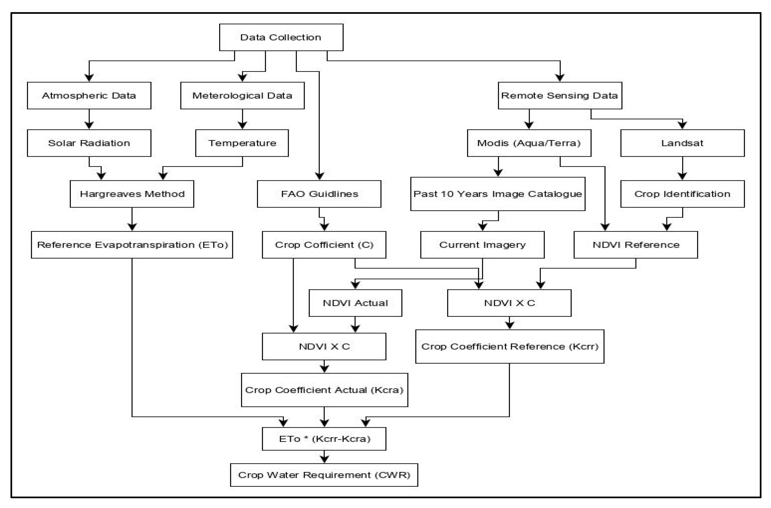
Crop water consumption, generally known as evapotranspiration (ET), can be calculated accurately at pixel level using remote sensing technology [13]. ET is the key parameter used for improvement in agriculture water management. Several methods are being used for direct or indirect measurement of crop ET; these include weighing lysimeter-based measurements, eddy covariance method, Bowen ration surface energy balance (BREB), surface energy balance algorithm for land (SEBAL), and using reference ET by multiplying it with crop coefficients [14]. Estimation of reference evapotranspiration based on crop coefficients is being used commonly for farm level agriculture management [6]. Reference evapotranspiration (ETo) is mostly calculated using weather parameters by common equations known as the Hargreaves equation and the Penman–Monteith equation. The Hargreaves equation requires minimum and maximum temperature as input for ETo calculation, while the Penman–Monteith equation requires temperature, wind speed, humidity, and sun radiation as input weather parameters [15]. ETo calculated through Penman–Monteith or Hargreaves equations reflect the values of a reference crop in ideally suited climate conditions and needs to be converted to crop specific consumption, i.e., actual evapotranspiration (ETa) using crop coefficients [9]. Crop coefficients reflect variable water need as per stage of the crop from sowing up to harvesting and vary for each crop as per its leaf area density and climate conditions [16].
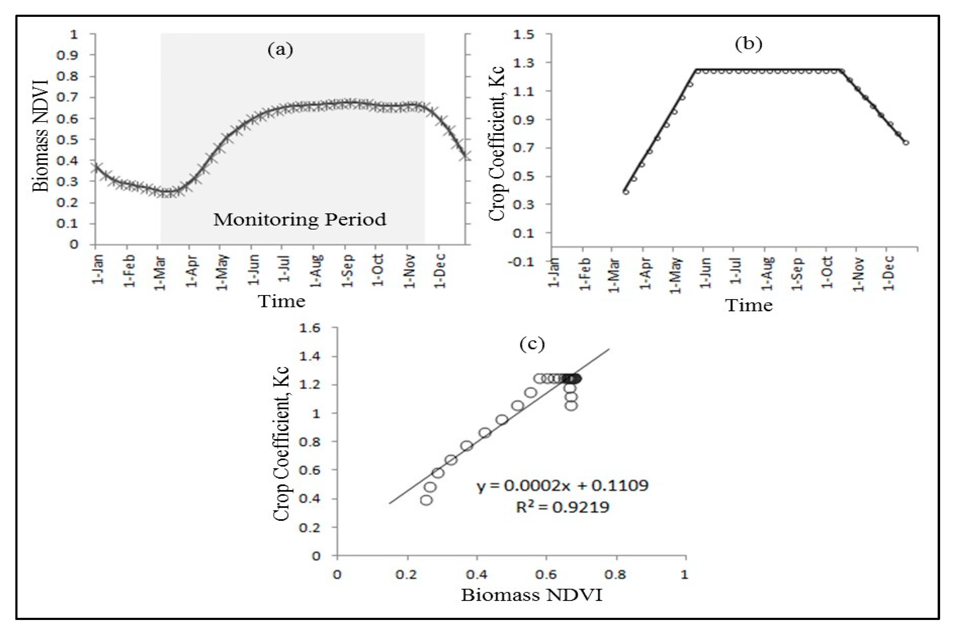
The crop coefficient approach is considered as reliable and efficient in determination of the spatiotemporal growth of crop water needs and crop specific variations show strong correlations with the satellite derived spectral index, normalized difference vegetation index (NDVI) [6,17,18,19]. Through regression calculation between crop coefficients and the NDVI, a set of crop specific parameters is created that allows the calculation of reflectance crop coefficients (Kcr) [17]. By applying Kcr to both, an ideal reference crop and the monitored crop, the difference between these two can be translated into crop water stress. This approach is quite significant as it provides crop coefficients (Kc) for each stage of the crop rather than providing a static estimate of Kc found in published reports or manuals. This method includes the data of land use for different dates throughout the crop growing season derived from the freely available satellite images of the whole year. This method is considered cost-effective in terms of data requirements, i.e., satellite images are available freely and climate data are available online in open access in comparison to the data collected through field surveys [20].
The spectral crop coefficient approach was used to monitor crop water consumption and to test the accuracy of crop coefficients for three fields in the Texas High Plains, all planted with cotton. Comparison was made of crop water use calculated from the reflectance-based crop coefficients approach and eddy covariance measurement approach (measured from a flux tower). In investigations, researchers used Landsat data for NDVI calculation, and ETo was calculated after the Penman-Monteith equation. They concluded that the use of reflectance crop coefficients is effective under a variety of different irrigation conditions and also stressed the adaptive character of the approach accounting for specific field conditions as opposed to standard crop coefficients [21]. NDVI-based Kc calculation approach is significant in crop water requirement estimation. The crop specific water requirements are expressed in terms of Kc and have been quantified for different crops. Water requirements can then be found through multiplying crop coefficients times the reference evapotranspiration [22,23,24,25,26]. Using modeled potential evapotranspiration (PET) and the relationship between NDVI and Kc, NDVI differences between ideal and monitored crop can be translated into irrigation water needs. Successful applications of this technique or approach have been reported in many studies and projects [25,26,27,28].
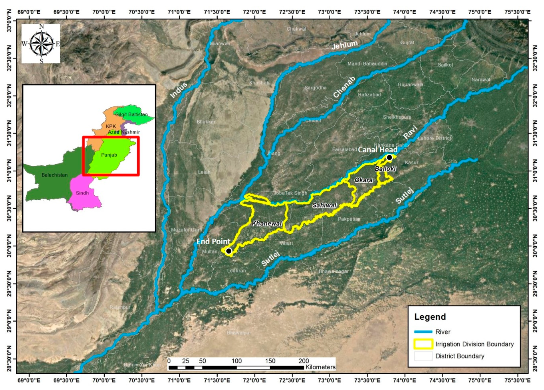
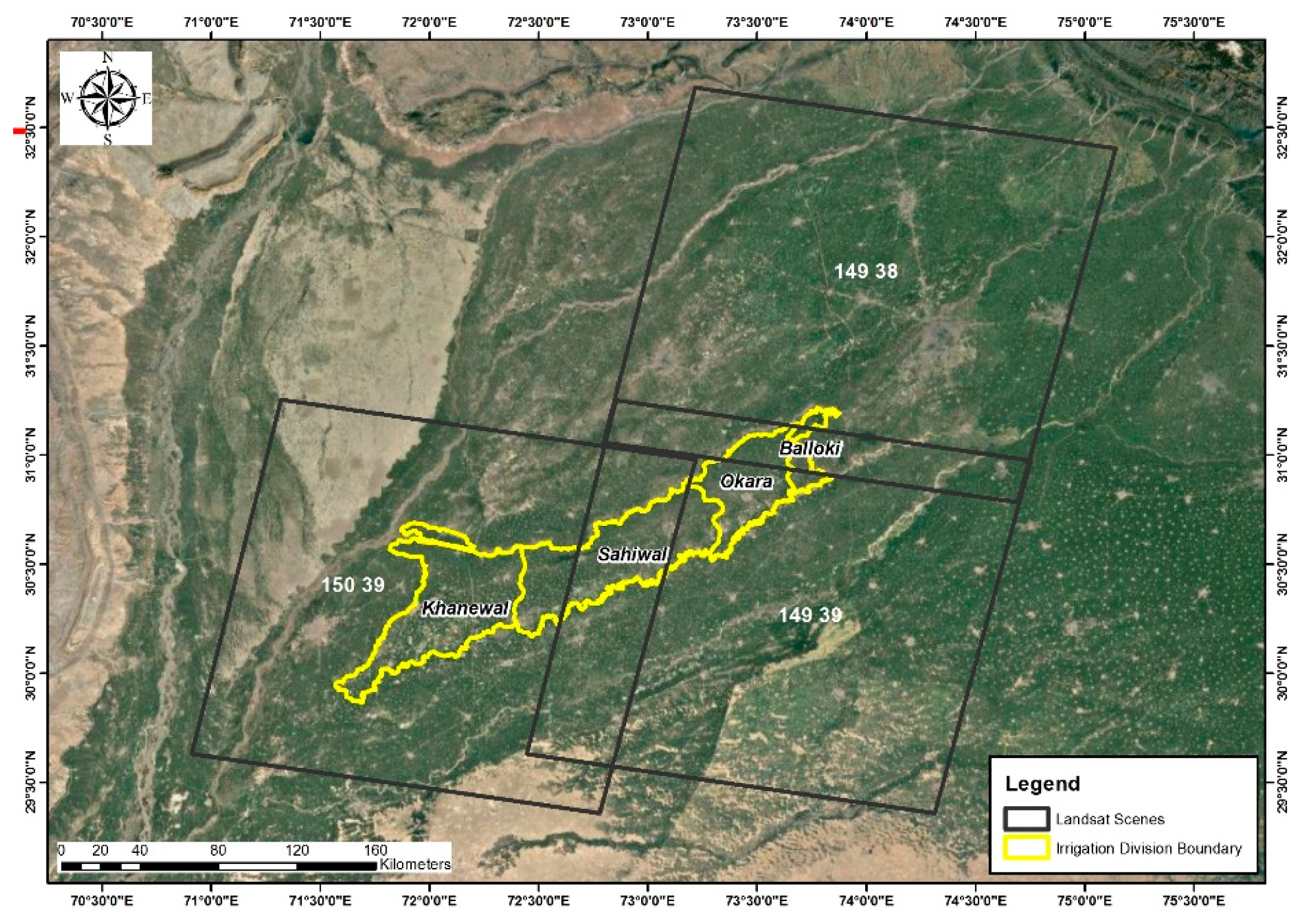
The purpose of this study is to provide the spatial distribution pattern of crop water requirement by monitoring the crop health in the Lower Bari Doab Canal (LBDC) command of the Punjab province. The results from this study would provide useful information for allocating water in main and secondary canals in order to avoid crop water stress and provide equitable water across the canal command. In summary, the objectives of this study are: (i) identification and quantification of different cropping patterns in LBDC; (ii) developing a decision support model for crop water efficacy at monthly intervals by using hydro-meteorological, geographical, and solar parameters; and (iii) scrutinizing the potential water deficit along the canal by counting upon the contribution of irrigation supplies and rainfall for both rabi and kharif seasons.

2. Materials and Methods

2.1. Study Area

The study area comprises four irrigation divisions, i.e., Balloki, Okara, Sahiwal, and Kahnewal, which are located in the longitudinal direction from the LBDC head. The climate of the study area is semi-arid. Mean daily maximum and minimum temperature varies between 32–36 °C and 11–15 °C, respectively. Temperature differs along the length of the canal command and gets warmer from east towards west. The mean yearly rainfall varies progressively from around 350 mm in the east to 200 mm in the west, the greater part of which falls in the storm, i.e., in the months of July and August. The winter precipitation generally occurs in the months of January and February in patches because of cyclonic storms from the south west. The winter season is gentle to chilly and stretches out from November to March [29]. Figure 1 describes the historical patterns of temperature and rainfall in study area for the years 2003–2012. The general slope of the territory is mild towards the south-west bearing, while the normal slope reaches from 1:4000 to 1:10,000. The LBDC canal command, overwhelmingly agricultural, lies at an altitude of 394–640 feet over the mean sea level. Texturally, the soil of the region is 70% medium (loam and sediment loam), 20% tolerably coarse (sandy soil and fine-sandy loam), 4% coarse (sandy and sandy loam), and 3% respectably fine (sandy-earth soil and silty-earth loam). The remaining 3% region possesses miscellaneous land types. The soils of the zone are intrinsically low in natural (organic) matter and accessible phosphorus [2,29].
LBDC originates from the Balloki headworks located southwest of Lahore, approximately 65 km apart, and ends in Khanewal division near Jahanian Tehsil as shown in Figure 2. A cultivable command area of about 1.7 million acres is being served by LBDC falling in the districts of Kasur, Okara, Sahiwal, and Khanewal. The design discharge of the canal is 9841 cusecs. The present carrying capacity of the canal is 8600 cusecs in the high flow season (June to August). The canal is usually not run on its designed capacity because of the shortage of water and also due to safety measures keeping in mind the old canal infrastructure [30]. Branch and distributary canals associated with the main LBDC are usually operated on a rotation basis to ensure equitable distribution of canal water. The rotation plan is prepared by each irrigation division at start of every cropping season by making groups of the canals based on their discharge, and priorities are fixed to release water on 8 daily bases. Generally, 3 groups are made of more or less equal discharge to rotate canals within a division, and each group gets its full share at least once every 24 days. The group falling in first priority gets full discharge, and remaining groups get a balanced share as per second or third priority fixed in the rotation plan [10]. There are approximately 275,000 farm families in this command area deriving their livelihoods directly from crop cultivation including wheat, maize, cotton, rice, flowers, vegetables, sugarcane, fodder, orchards, and citrus crops. The LBDC command area is considered as progressive and an important agriculture area in Punjab province and provides substantial potential for increased productivity. Wheat has the major share amongst all the crops in study area, while cotton and maize have the second and third largest share, respectively [30].

2.2. Data Collection

Multiple datasets were collected from different sources to be used to demonstrate the crop water deficit in the LBDC area. Hydrometeorology, irrigation, and remote sensing satellite information collected from different sources including organizational and open-source platforms were pre-processed in a GIS environment (Table 1). However, methodological flowchart of the research is shown in Figure 3.

2.3. Data Processing

The methodology used the concept of reference evapotranspiration (ETo) at a spatiotemporal scale. The empirical approach of the Hargreaves method has been used for the estimation of ETo in the LBDC command area. The Food and Agriculture Organization (FAO) of the United Nations proposed the Penman-Monteith equation, Equation (1), as the standard method for estimating ETo. The Penman-Monteith equation requires multiple climate parameters, which were not available with weather stations existing in the study area on the required frequency that hence could have yielded wide gaps and/or inaccuracies in ETo estimation. To solve this problem, the Hargreaves equation (HARG) is recognized by FAO and is often used in data poor areas. The Hargreaves equation is based on average, minimum, and maximum air temperature and extraterrestrial radiation. It tends to overestimate ETo in humid conditions and requires a local calibration. Moreover, this approach is simple and effective and can be used for daily seasonal and monthly calculations of ETo [31,32,33].
Different schemes have been employed for calculation of ETo, and the Hargreaves method was observed to be simple and highly correlated for seasonal and daily bases [34]. The mathematical equation of ETo calculation is given as:
E T o = 0.0023 × ( T m a x + T m i n 2 + 17.8 ) × T m a x T m i n
where, T-max(°C) and T-min(°C) are average daily maximum and minimum temperatures, respectively, and R is extra-terrestrial solar radiation.
Daily temperature data available for weather stations located inside the LBDC region were used to calculate the ETo. To get the ETo monthly measurements, monthly mean temperatures were supposed to resemble that of an average monthly day, so Equation (1) was applied, and then result was multiplied by the total number of days of the corresponding month. Afterwards, for spatial interpolation of ETo, inverse distance weight (IDW) was chosen over other complex methods (e.g., cokriging) that gave unsatisfactory results. This operation provides the spatial distribution of ETo at monthly intervals [35].
However, among the meteorological information, rainfall data were collected from the open-source platform of NASA (National Aeronautics and Space Administration: Earth Data). GPM (Global Precipitation Mission) and TRMM (Tropical Rainfall Measurement Mission) datasets were collected at daily temporal resolution and processed to monthly information. All information was standardized at the same scale and was restricted to the irrigation division level of LBDC command area. The datasets were pre-processed and resampled, if needed, for monthly calculation of crop water requirements for winter (rabi) and summer (kharif) seasons.

2.4. Crop Classification

For accurate quantification of water requirement and consumption, crops were classified into two seasons: rabi (winter) crops and kharif (summer) crops. This required a differentiation of major crop types grown in a calendar year. The crop pattern in the study area was identified using Landsat satellite imagery. The product was used for its free availability and reasonable spatial, spectral, and temporal resolution. The time series NDVI is widely considered as a reflection of crop phenology [36]. NDVI time series were calculated from near infrared and red bands of Landsat, and the phonological shapes were used for crop identification. To cover the LBDC area, two Landsat footprints/tiles (Path 149 Row 39 and Path 150 Row 39 as shown in Figure 4) were processed under the object-based classification algorithm (OBCA).
A small part of the Balloki division was lying in the 3rd tile of Landsat (Path 149 Row 38); however, it was stitched with the corresponding tile (Path 149 Row 39). For the composition of NDVI time series, each footprint was processed using 21 Landsat time series images of years 2013–2014.
The stacked NDVI of the study area was used for pattern generation representing the crop phenology throughout the year. Each crop behaves differently in NDVI representing cycles. The clusters of different vegetation covers are grouped in the remote sensing environment to generate the crop pattern in the area. The classification technique using NDVI series is used by different researchers and has been found efficient for crop type mapping and monitoring [6,18,19,37]. Specimens of NDVI-based phonological profiles of wheat and cotton crops are shown in Figure 5 and Figure 6, respectively.

2.5. MODIS, NDVI and Reference Crop Cycle

NDVI is an index that evaluates biomass calculated from a near infrared band and a red band. The NDVI product of MODIS (AQUA/TERRA) is used for reference crop cycle generation. The reference crop cycle defines the maximum value of crop reflectance observed in past 10 years. These cycles of individual crops behave near ideally throughout the season from crop sowing to harvesting stage. To meet the optimum condition, it was of the utmost importance to minimize the data gaps. MODIS provides NDVI from two platforms: AQUA and TERA. These platforms deliver NDVI imagery with an offset of 16 days, however, harmonizing the two dataset results in 8 daily by-products of NDVI. These NDVI images are stacked over a period of 10 years for reference cycle identification using Fourier filter technique.

2.6. Crop Coefficients (Kc) and Crop Water Requirement

Crop coefficients have a strong correlation with satellite derived NDVI values, and both are directly proportional to each other. Reflectance-based crop coefficients (Kcr) are calculated through linear regression between NDVI and FAO defined crop coefficients (Kc) values [6]. The shaded grey area in Figure 7a represents NDVI values included in the linear regression of sugarcane crop, and Figure 7b represents corresponding FAO defined Kc values. After applying the linear regression, the resultant coefficients named C1 and C2 were determined for calculation of reflected crop coefficients (Kcr) as shown in Figure 7c. The linear equation 2 used for Kcr calculation for both the monitoring period and reference crop period is given below.
K c r = C 1 × N D V I + C 2
The C1 and C2 coefficients are crop specific and were determined individually. However, there exist generally applicable C1 and C2 variables also [6]. The reflectance-based Kcr were generated for reference (ideal) crop cycle and actual NDVI collected at 8 daily intervals. Kcr of both actual and reference NDVI were then translated to crop water deficit calculation using the following Equation (3):
C W R = ( K c r r K c r a ) × E T o

3. Results

3.1. Cropping Pattern in LBDC

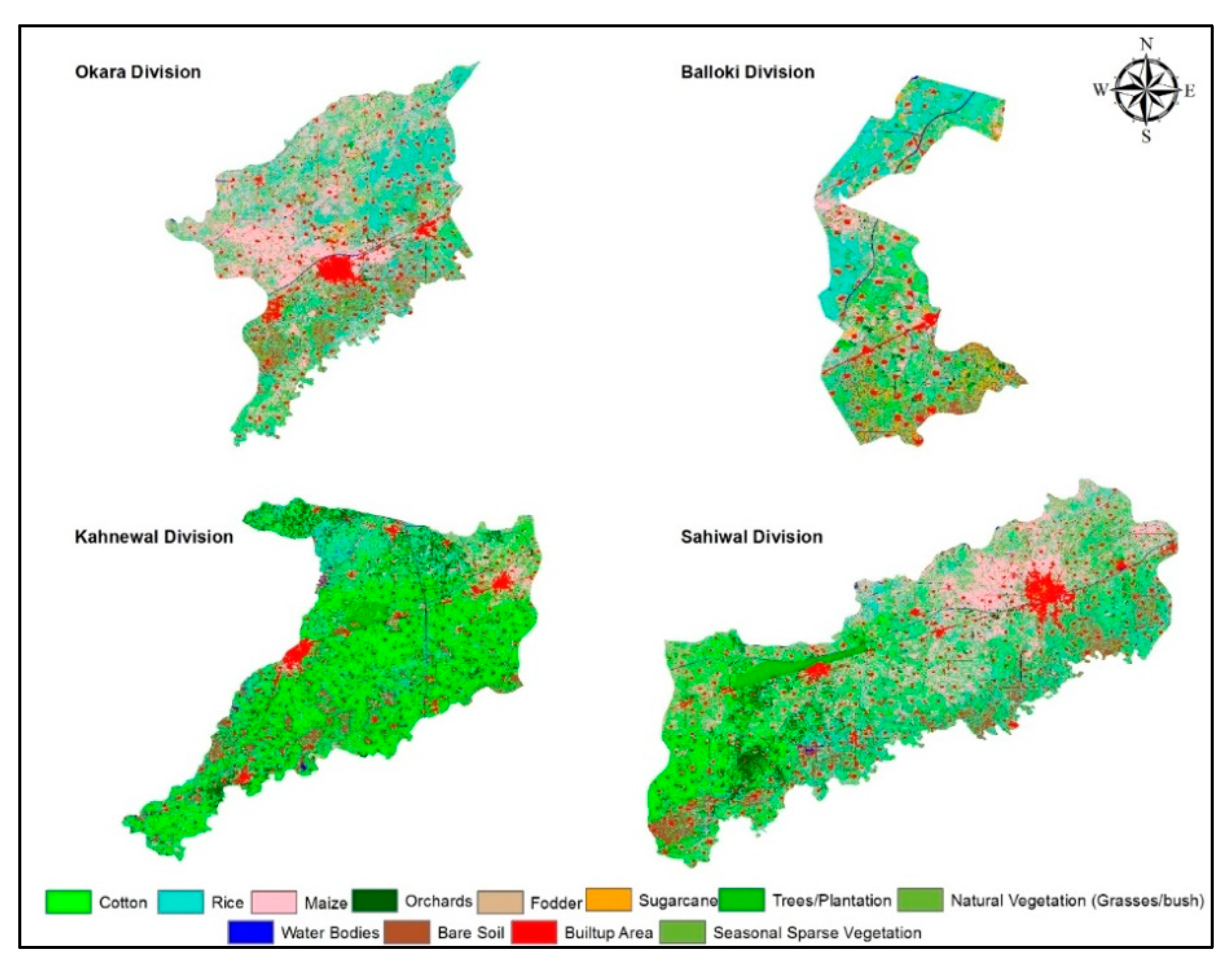
The vegetation index (NDVI) time series approach generates a total number of 12 land covers in the study area including six crop types. The classification scheme follows the crop calendar and defines summer (rabi) and winter (kharif) season crops separately.
The time series NDVI profiles of each class behave differently due to the intrinsic properties of crops. For example, wheat and rice are the perennial crops of rabi and kharif seasons substantiated in the study area, respectively. The NDVI profiles of both crops are closely related to each other, but the seasonal crop calendar (sowing and harvesting dates) is completely different. However, different weather conditions may lead to slight variations in the NDVI profile of same crops among different years. The results show that wheat, maize, and potato crops cover a major portion for rabi season in the LBDC region illustrated in Figure 8.
On the other hand, maize and cotton are the major crops of the kharif season as shown in Figure 9. The area comprises a combination of perennial and non-perennial crops as shown in Table 2.
Spatial distribution shows that the northeast (NE) region of the LBDC command comprises maize; however, a huge concentration of cotton was found while moving towards the southern side of the area. The spatial distribution describing rice, fodder, and sugarcane classes covering small portions in the study area as shown in Figure 8 and Figure 9.

3.2. Crop Calendar and Coefficients of LBDC

The sowing and harvesting periods and stages are different for different spatial extents. However, the LBDC area comprises a large spatial extent and has variable stages of crops. The annual crop cycles for each crop in the study area were collected from the field survey and by considering the local expert knowledge. The crop calendar describes the temporal variation of individual crop growth over a year in the study area. Different stages of crops according to their sowing and harvesting time periods are presented in 
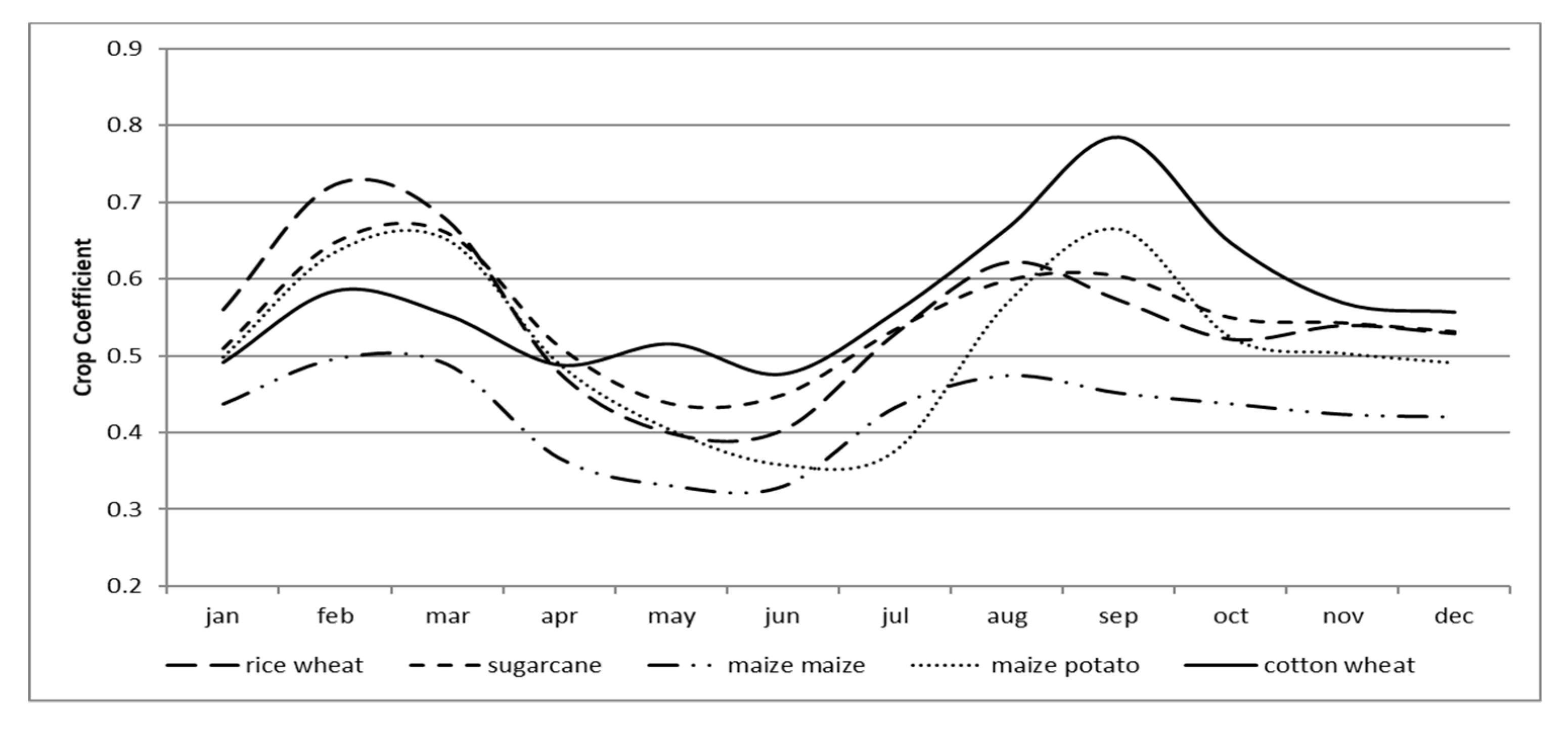
Table 3. The reflection-based crop coefficients (Kcr) were generated for individual crops using Equation (2). The average Kcr values of individual crops for years 2014–2016 are shown below in Figure 10.
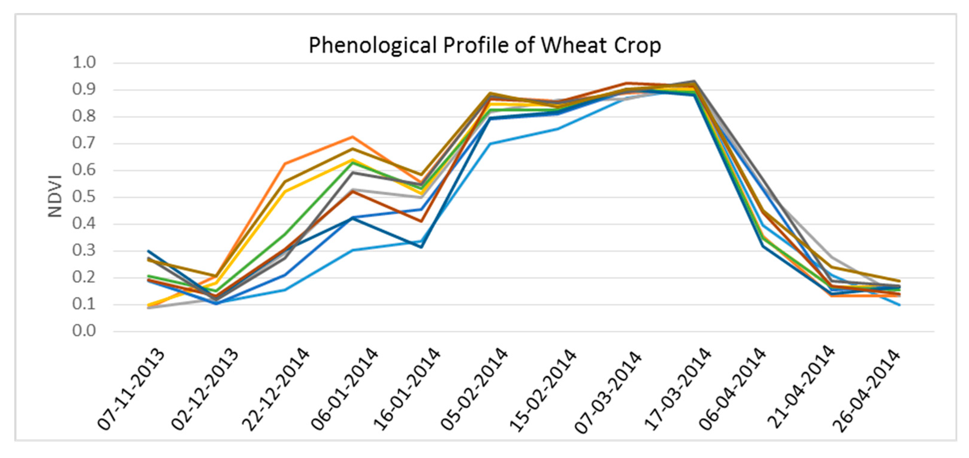
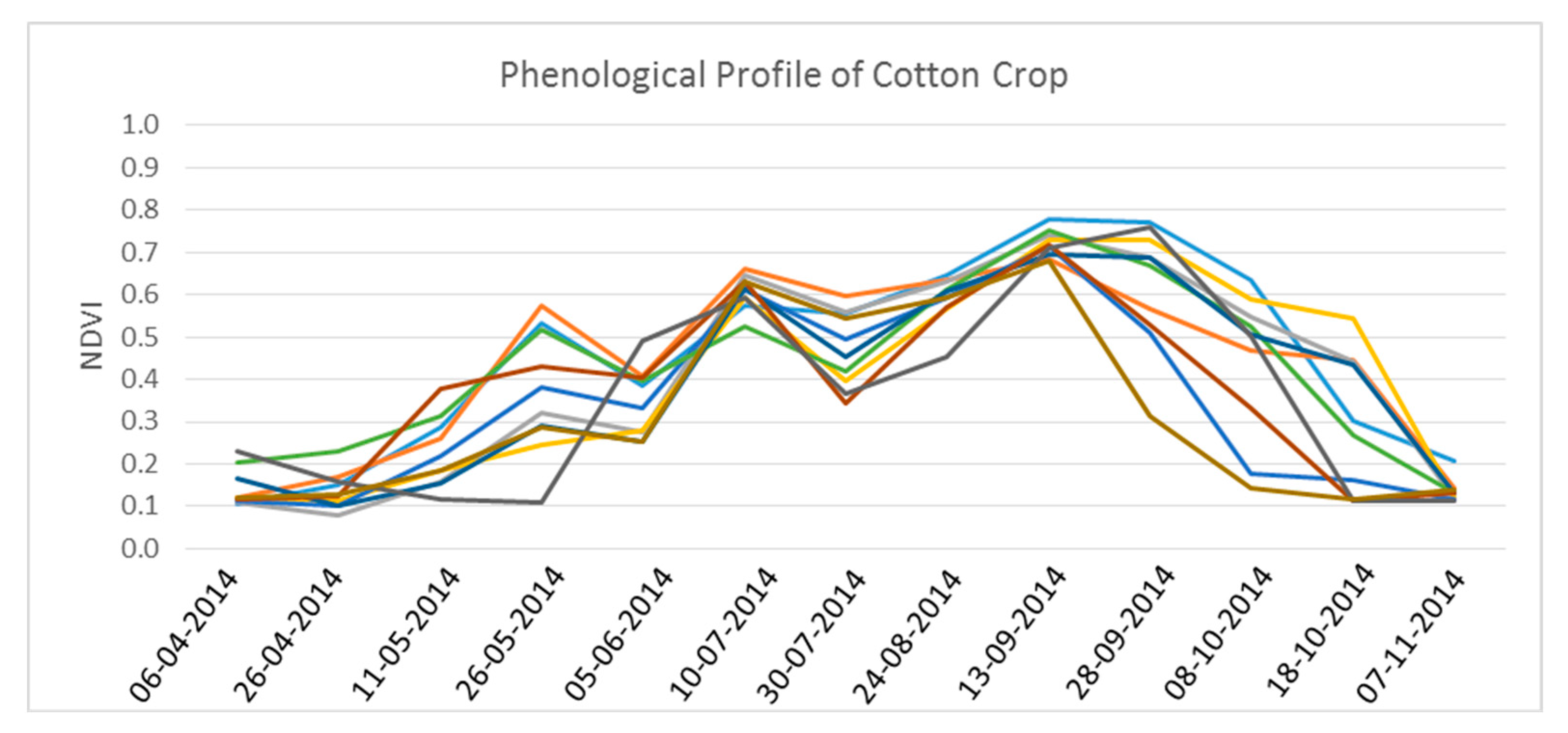
The smaller NDVI values resulted in smaller Kc values and vice versa. The maximum value of Kc for each crop was observed between the middle to final stage whereas the initial stage reflected a low value. For instance, following the rice–wheat crop combination, the Kc value curve attains maximum value for wheat crop in the months of February (middle) and March (final stage). However, the same line goes to minimum in the months of May and June when wheat is harvested, and it again starts to climb when rice is cultivated. It again attains peak and goes to bottom after the harvesting of rice. The same is the case with other crop combinations corresponding to their sowing and harvesting periods. The case of sugarcane is different as it is considered a whole year crop, and its Kc curve attains peak value depending upon its sowing period.
The reflection-based Kc trend corresponded with the stages of crops (initial, middle, and final stages) tabulated in the crop calendar as shown in Table 3, which was prepared using crop phonological profile. Crop calendar was also verified during field survey by interviewing farmers.

3.3. Spatial Distribution of Meteorological Parameters (ETo, T, and P)

Temperature, evapotranspiration, and precipitation are very crucial parameters in calculation of crop water requirement. The parameters for the quantification of water deficit are used on a monthly basis for the years 2014, 2015, and 2016. 
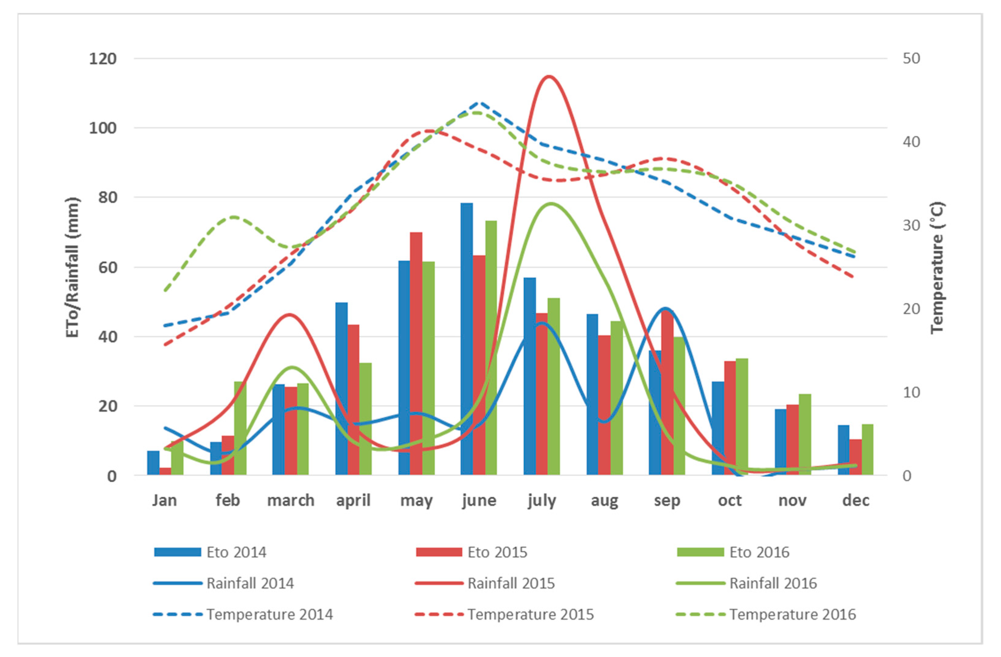
Figure 11 shows the variation of evapotranspiration, temperature, and rainfall for the years 2014, 2015, and 2016.
The results show that high values of evapotranspiration, temperature, and rainfall lie between the months April-August, April–September, and July–September, respectively, for the years 2014, 2015 and 2016. Maximum values of evapotranspiration and rainfall were observed in the months of June and July, respectively. These two parameters are in inverse relation to each other by indicating a decreasing trend of ETo compared to the rise in rainfall in the month of July. However, with the increase in temperature, the values of evapotranspiration also increased as shown in Figure 11, which indicates a positive relation between the two parameters.
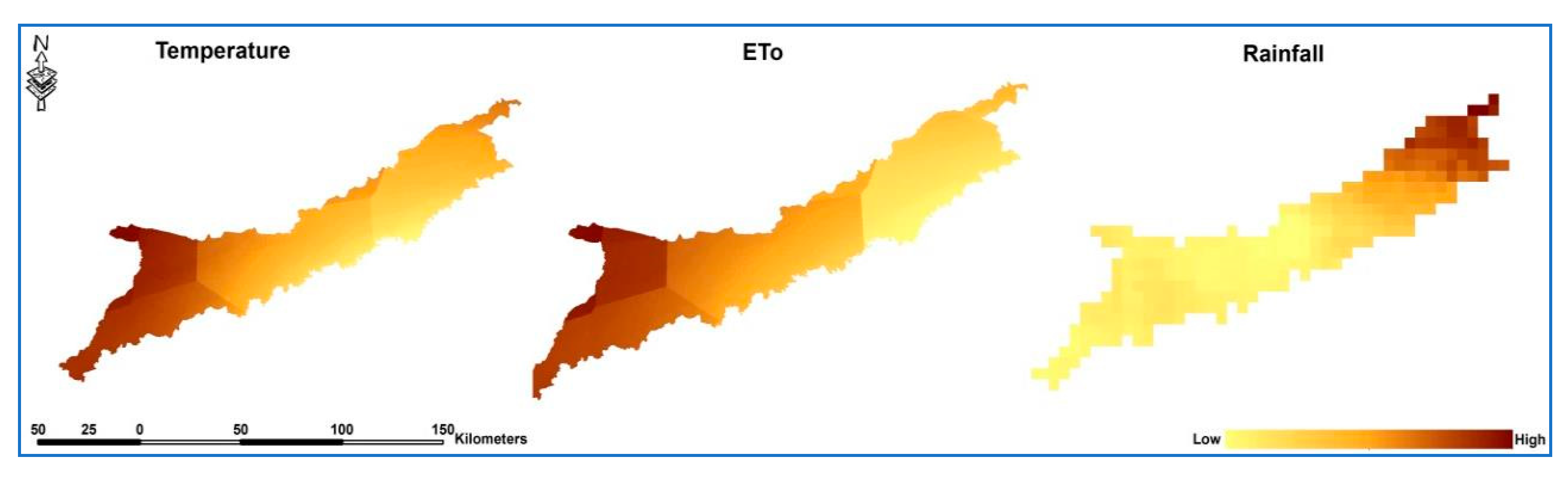
Chronological behavior of evapotranspiration, temperature, and rainfall shows variability in the spatial distribution pattern in LBDC as shown in Figure 12. It has been observed that temperature and evapotranspiration have an increasing trend from east towards west in the study area. On the contrary, precipitation has a decreasing trend moving from west towards east. In general, similar pattern and correlation between evapotranspiration and temperature parameters have been observed for all the months of three years in the study area.

3.4. Crop Water Deficit and Requirement

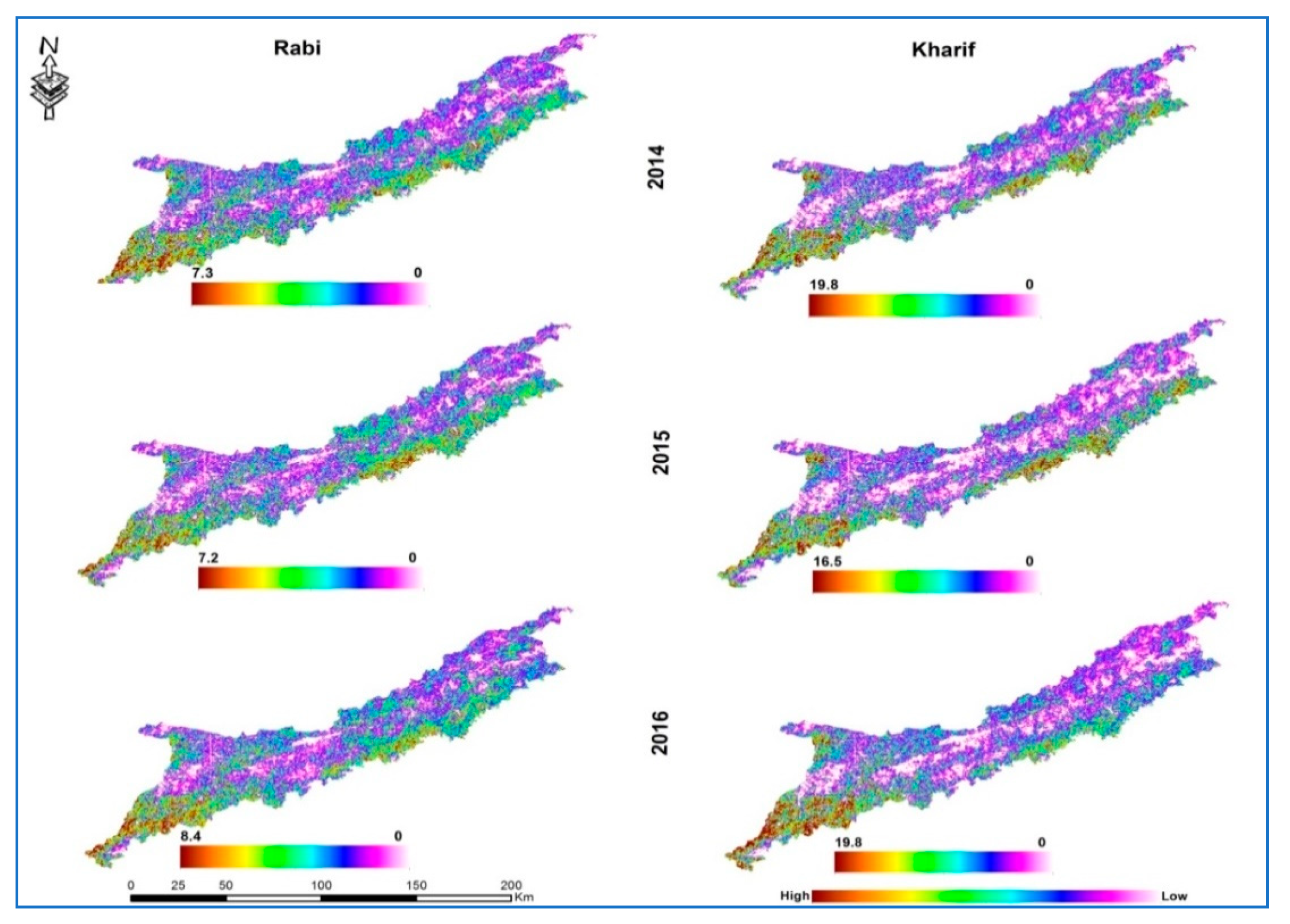
The incorporated meteorological parameters and crop cycles resulted in chronological crop water deficit assessment in the LBDC region. Seasonal mean water deficit for the years 2014, 2015, and 2016 has been mapped in the study area as shown in Figure 13. It depicts the spatial distribution pattern of water deficit for rabi and kharif seasons in millimeters. Generally, the same spatial distribution pattern of water deficit for rabi and kharif seasons was observed in the study area. However, a deficit value in the kharif season is much higher than rabi season for all three years. This is because the kharif season lies in the hottest months of the year (i.e., June and July), which causes maximum evapotranspiration resulting in high water deficit.
Figure 13 illustrates extremely high deficit observed at the tail (southwest) of the study area due to less irrigation supply because of maximum conveyance losses occurring and being located far away from the canal head. Similarly, southeast parts show high deficit for both seasons of these three years. These areas also lie along the border of the canal command and at the tail of the secondary canals, whereas northeast and northwest parts face considerably less deficit due to the advantage of lying close to the canal head and near to the Ravi river.
Irrigation supply, groundwater, and rainfall are the available sources to fulfill the crop water needs. However, groundwater pumping is not feasible or available for all farmers on demand, and small land holders usually rely on canal supply and rainfall. Influence and correlation of irrigation supply and rainfall parameters with crop water deficit measured on a monthly basis in LBDC are shown in Figure 14.
The results show that less than 10 mm mean deficit is observed in the winter months (October-February) for the years 2014, 2015, and 2016. The low values of water deficits are mainly due to the lower evapotranspiration rate because of temperature falling down in these months. Specifically, December and January show relatively the least deficit due to the teleconnection of water deficit with evapotranspiration and temperature. Irrigation supply is not available in the months of January due to annual canal closure, but rainfall has supplemented to fill the gap. The crop calendar and trend graph of Kc also complement the deficit result because rabi crops are at an initial stage of their growth period during these months and require a substantially lower amount of water as shown in Figure 15.
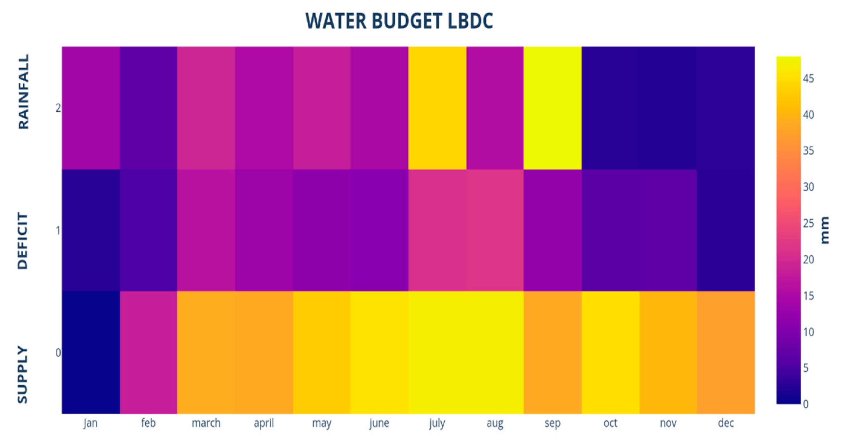
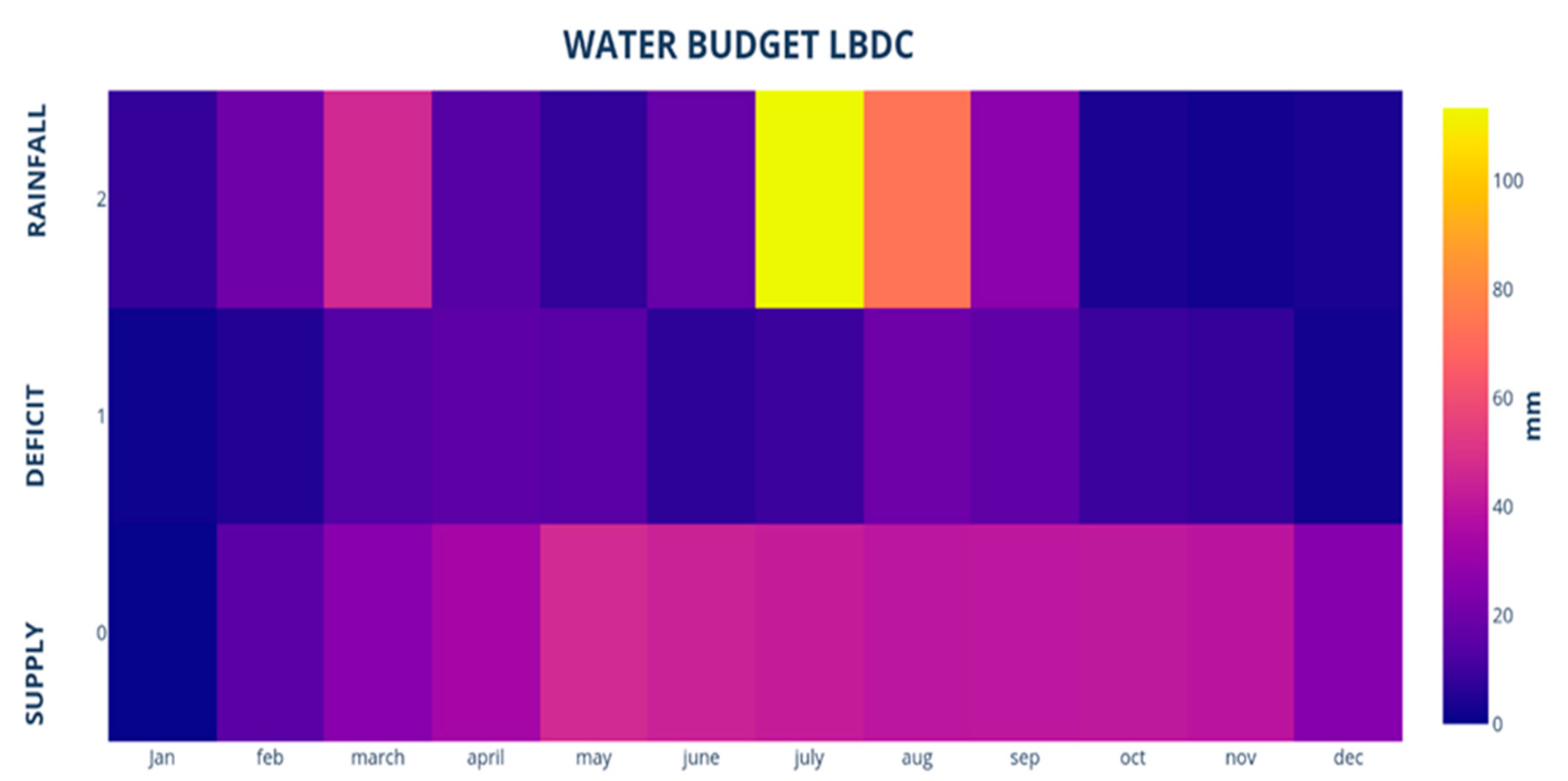
The annual cycle of water budget for 2014 (Figure 15) shows that more than 40 mm of irrigation water was supplied to the LBDC throughout the year except for the months of January and February. This constant volume of canal supply is not sufficient for the crops in the peak summer months of July and August. Although aid of precipitation, around 45 mm, was available in the month of July, it was not able to meet the crop demand. However, it is obvious that when the peak summer months were over and temperature started to fall in the month of September, rainfall was also available in a good proportion of 50 mm, the deficit fell considerably. The deficit values dropped to a range of 5–10 mm from the month of October onwards because of the sufficient decrease in Kc values, hence low water requirement of crops.
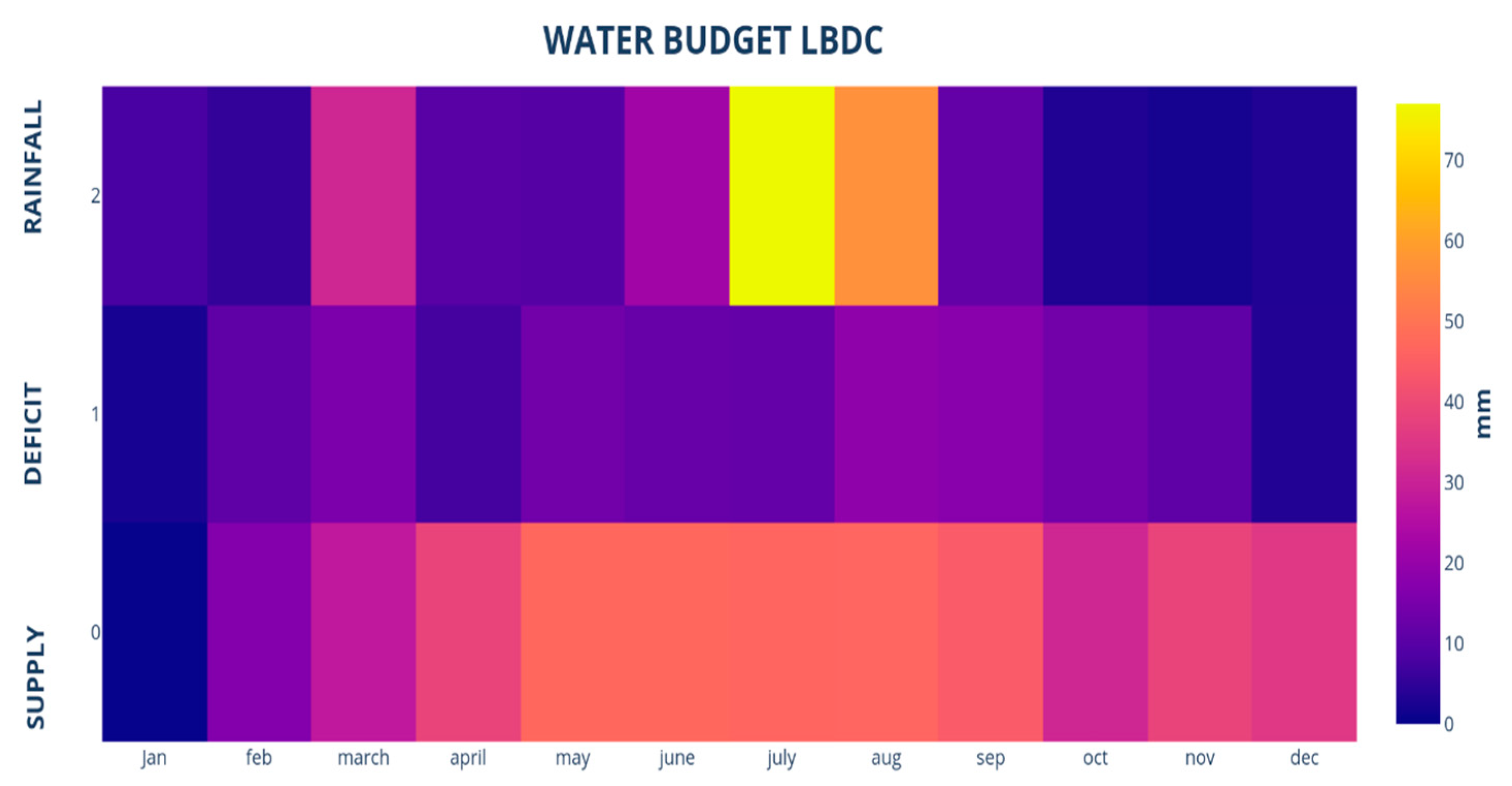
In the water budget graph of the year 2015 (Figure 16), water deficit did not attain peaks in peak summer months of June to August, because the LBDC command area received high precipitation in these months. It was observed that a very high value of rainfall (>100 mm) for the month of July restricted the deficit to as low as 5 mm. However, the irrigation supply remained in the range of 40–45 mm for April-November. It is obvious from the water budget graph of the year 2015 that rainfall volume in the study area directly influences the crop water deficit. The water deficit pattern in the winter months is much more similar to the year 2014.
Similar rainfall and irrigation supply patterns were observed in the year 2016 as shown in Figure 17. However, rabi crops are observed with a shortage of water in the peak demand month of March due to a lower amount of rainfall as compared to years 2014 and 2015. High volume of rainfall in June and July for the kharif season kept the deficit under control, similar to the year 2015.
From results of all three years, the fact is established that the study area observes relatively high water deficit in the kharif season due to higher temperature, which causes maximum evapotranspiration in the months of June, July, and August. Although irrigation supply remains relatively high during these kharif months, crop demand is not satisfied unless sufficient volume of precipitation is available or groundwater is pumped in ample proportions. For the rabi season, the months of March and April are critical to meet crop water demand because of wheat being the dominant crop at its peak growth. Moreover, increase in ET values and decline in precipitation during peak demand months of rabi and kharif seasons favor water deficit in crops. On the contrary, the months of December, January, and February, being the coolest months of the year, face minimal ET deficit in the study area because crop water demand is fulfilled by the precipitation and irrigation supply and groundwater abstraction.

4. Discussion

Canal water scarcity and inefficient management of irrigation water channels are resulting in maximization of the use of groundwater to fulfill the crop water needs. Groundwater pumping is at maximum during the driest months of the year because of the higher rate of evapotranspiration. This fact is also confirmed in different published research that shows that in south Asia, Pakistan is the country with the highest groundwater usage of around 53% [38]. It is imperative to improve crop water allocation by identifying the particular cropland under stress in irrigation districts and disseminating it to canal managers and farmers in a timely manner. Visualizing the impact of spatial precipitation variations is necessary to rationalize canal water allocation, which is possible by establishing an approach that is capable of providing estimation of the spatiotemporal dissemination of crop water requirements [39]. Availability of spatial and temporal crop distribution data is one of the major components in devising policies for the agriculture sector regarding sustainable irrigation water management. A decision support tool for water resources management should be developed by acquiring the understanding of agricultural practices and the availability of reliable assessments of crop water requirements [40]. Particular challenges in the development of a crop water management system are the size of the Punjab irrigation area, spatial and temporal crop variability, the location specific stress situation of crops that cannot be compared to standard crops, and the developmental status of technically viable monitoring techniques/models. Spatial analyses at such scale and at such short repetitive steps are only feasible with remotely sensed images.
This pilot research study attempts to provide a cost- and time-effective approach for efficient monitoring of crop health over one of the largest canal command areas in Punjab, Pakistan. The major goal of this study was to develop a spatial decision support tool to integrate and standardize the various parameters for estimation of crop water needs. Multiple datasets including hydrometeorology, irrigation, and remote sensing satellite information collected from different sources including organizational and open-source platforms were employed in GIS and remote sensing environments. Reference evapotranspiration (ETo) and crop coefficients were of major concern for quantification of crop water requirements in the study area. The Hargreaves method, considered as simple and reliable, especially in data poor areas, has been employed for calculation of reference evapotranspiration (ETo) [35,41], while reflected crop coefficients (Kcr), which proved highly correlated with the NDVIs, were derived using MODIS NDVI product and FAO defined crop coefficients (Kc) for calculation of reference and actual crop coefficients [42]. Crop type and pattern were identified using Landsat imagery for accurate crop water quantification.
The research results verified the worth of satellite data for proficient appraisal of crop health monitoring. They also highlighted the worth of open-source information for crop water requirement estimation. The multi-step scheme for near real-time irrigation water stress estimation is quite effective in nature for large scale studies with limited data availability and therefore could be employed on other regions of the same agro-climatic conditions.

5. Conclusions

This study presents a technique for crop water deficit modeling in data poor areas and concluded the following:
(i) NDVI-based crop classification revealed that wheat and cotton are the major cultivated crops for rabi and kharif seasons with an area of approximately 60% and 30%, respectively. However, maize crop is non-perennial in nature, showing a variable cultivated area in rabi and kharif seasons. Sugarcane and rice, being the perennial and non-perennial crops, respectively, are also cultivated in a small portion of the study area. It is clear from the crop statistics that the kharif season has more variation in crop cover than the rabi season, hence requiring more dynamic water allocation.
(ii) The reflection-based Kc values remained consistent with crop calendar of LBDC generated by the local experts and published reports. The Kc values remained high at middle and final stages for both rabi and kharif season crops due to the maximum NDVI value, hence maximum crop water requirement at these stages.
(iii) The LBDC command area receives a continuous canal water supply throughout the year, except the month of January, which is observed as the annual canal closure. A relatively low volume of rainfall, i.e., 50 mm, was observed in July 2014, which caused the deficit to rise up to 30 mm in July, one of the hottest months, while the year 2015 received higher rainfall, especially in July, of up to 120 mm, minimizing the deficit to as low as 5 mm. However, the study area received 80 mm rainfall in July for the year 2016, and the deficit climbed up to 40 mm because of relatively low rainfall accompanied with a reduction in irrigation supplies due to maintenance work going on in LBDC [8].
(iv) The consumptive use of irrigation supply and groundwater is vital to meet crop water needs, though consumptive use is still not able to meet crop demand as observed in the results. However, the rainfall pattern directly influences the quantitative behavior of the deficit. The research results endorsed the water budget published by the On Farm Water Management (OFWM) Agriculture Department that stated that groundwater and irrigation supply are not sufficient to meet crop demand in the LBDC, and rainfall plays an important role especially in the summer to reduce deficit. Moreover, the deficit values remained high in March and April for rabi crops and in August and September for kharif crops due to the high crop water demand. Water deficit was observed to be consistent towards the tail end of the main canal and secondary canals, which needs to be addressed to ensure equitable distribution of irrigation water resources.
There is a dire need to use modern technology of remote sensing and GIS to efficiently utilize irrigation water resources and avoid crop water stress by monitoring crop health and climate conditions simultaneously. A spatial decision support system (SPSS) needs to be developed for better management of canal water and alternate sources available for crop water use. The current study has laid the foundations for using independent and open-source technology to monitor crop water stress on a near real-time basis and guide decision makers to take informed decisions.

Author Contributions

Conceptualization: M.A.J., S.R.A., W.K.A., B.A.M.; Analysis: M.A.J., W.K.A., B.A.M.; Writing—Original Draft Preparation: M.A.J., S.R.A.; Writing—Review & Editing: B.A.M., M.A.J., S.R.A., W.K.A. All authors have read and agreed to the published version of the manuscript.

Funding

This research received no external funding.

Acknowledgments

The authors would like to acknowledge the Punjab Irrigation Department for providing irrigation discharge and crop samples for LULC validation.

Conflicts of Interest

The authors declare no conflict of interest.

References

  1. FAO’s Global Information System on Water and Agriculture. Available online: http://www.fao.org/aquastat/en/overview/methodology/water-use (accessed on 1 November 2019).
  2. Ashraf, M.; Nasir, A.; Saeed, M.M. Evaluation of the existing water productivity in the Lower Bari Doab Canal (LBDC) command—A case study. Pak. J. Agric. Sci. 2010, 47, 389–397. [Google Scholar]
  3. Siyar, M.; Khan, A.S.; Rahman, F. Spatio-temporal Assessment of Productivity in Pehur Main Canal System, Pakistan. Proc. Pak. Acad. Sci. A Phys. Comput. Sci. 2018, 55, 9–18. [Google Scholar]
  4. Mullick, M.R.A.; Khattak, M.S.; Haq, Z.U. Considering environmental flow for water resources management in South Asia: Current status and challenges. J. Eng. Appl. Sci. 2012, 31, 37–44. [Google Scholar]
  5. Bhavsar, P.N.; Patel, J.N. Development of relationship between crop coefficient and NDVI using geospatial technology. J. Agrometeorol. 2016, 18, 261. [Google Scholar]
  6. Kamble, B.; Kilic, A.; Hubbard, K. Estimating crop coefficients using remote sensing-based vegetation index. Remote Sens. 2013, 5, 1588–1602. [Google Scholar] [CrossRef] [Green Version]
  7. Qureshi, A.S.; Gill, M.A.; Sarwar, A. Sustainable groundwater management in Pakistan: Challenges and opportunities. Irrig. Drain. J. Int. Comm. Irrig. Drain. 2010, 59, 107–116. [Google Scholar] [CrossRef]
  8. On Farm Management. Directorate General Agriculture, Lahore, Pakistan. Available online: http://www.ofwm.agripunjab.gov.pk/ (accessed on 5 November 2019).
  9. Irrigation Department Punajb, Lahore, Pakistan. Available online: http://www.irrigation.punjab.gov.pk/ (accessed on 9 November 2019).
  10. Ministry of Food, Agriculture and Livestock, Pakistan. Water Development for Irrigated Agriculture in Pakistan: Past Trends, Returns and Future Requirements FAO 2002; Ministry of Food, Agriculture and Livestock: Islamabad, Pakistan, 2002.
  11. Basharat, M.; Tariq, A.R. Command-scale integrated water management in response to spatial climate variability in Lower Bari Doab Canal irrigation system. Water Policy 2014, 16, 374–396. [Google Scholar] [CrossRef]
  12. Hatfield, J.L.; Dold, C. Water-use efficiency: Advances and challenges in a changing climate. Front. Plant Sci. 2019, 10, 103. [Google Scholar] [CrossRef] [Green Version]
  13. Dhungel, S.; Barber, M.E. Estimating Calibration Variability in Evapotranspiration Derived from a Satellite-Based Energy Balance Model. Remote Sens. 2018, 10, 1695. [Google Scholar] [CrossRef] [Green Version]
  14. Mkhwanazi, M.; Chavez, J.L.; Andales, A.A. SEBAL-A: A remote sensing ET algorithm that accounts for advection with limited data. Part I: Development and validation. Remote Sens. 2015, 7, 15046–15067. [Google Scholar] [CrossRef] [Green Version]
  15. Allen, R.G. Crop Evapotranspiration-Guideline for computing crop water requirements. Irrig. Drain. 1998, 56, 300. [Google Scholar]
  16. Allen, R.; Irmak, A.; Trezza, R.; Hendrickx, J.M.; Bastiaanssen, W.; Kjaersgaard, J. Satellite-based ET estimation in agriculture using SEBAL and METRIC. Hydrol. Process. 2011, 25, 4011–4027. [Google Scholar] [CrossRef]
  17. Bendig, J.; Bolten, A.; Bennertz, S.; Broscheit, J.; Eichfuss, S.; Bareth, G. Estimating biomass of barley using crop surface models (CSMs) derived from UAV-based RGB imaging. Remote Sens. 2014, 6, 10395–10412. [Google Scholar] [CrossRef] [Green Version]
  18. Glenn, E.P.; Neale, C.M.U.; Hunsaker, D.J.; Nagler, P.L. Vegetation index-based crop coefficients to estimate evapotranspiration by remote sensing in agricultural and natural ecosystems. Hydrol. Process. 2011, 25, 4050–4062. [Google Scholar] [CrossRef]
  19. Rossi, S.; Bocchi, S. Monitoring crop evapotranspiration with time series of MODIS satellite data in Northern Italy. In New Developments and Challenges in Remote Sensing; Millpress: Rotterdam, The Netherlands, 2007. [Google Scholar]
  20. Long, D.; Singh, V.P. Assessing the impact of end-member selection on the accuracy of satellite-based spatial variability models for actual evapotranspiration estimation. Water Resour. Res. 2013, 49, 2601–2618. [Google Scholar] [CrossRef]
  21. Rajan, N.; Maas, S.J. Spectral Crop Coefficient Approach for Estimating Daily Crop Water Use. Adv. Remote Sens. 2014, 3, 197–207. [Google Scholar] [CrossRef] [Green Version]
  22. Ferreira, M.I.; Conceição, N.; Malheiro, A.C.; Silvestre, J.M.; Silva, R.M. Water stress indicators and stress functions to calculate soil water depletion in deficit irrigated grapevine and kiwi. In Proceedings of the VIII International Symposium on Irrigation of Horticultural Cropsleida, Lleida, Spain, 8–11 June 2015; Volume 1150, pp. 119–126. [Google Scholar]
  23. Navarro, A.; Rolim, J.; Miguel, I.; Catalão, J.; Silva, J.; Painho, M.; Vekerdy, Z. Crop monitoring based on SPOT-5 take-5 and Sentinel-1A data for the estimation of crop water requirements. Remote Sens. 2016, 8, 525. [Google Scholar] [CrossRef] [Green Version]
  24. Baup, F.; Villa, L.; Fieuzal, R.; Ameline, M. Sensitivity of X-Band (σ0, γ) and Optical (NDVI) Satellite Data to Corn Biophysical Parameters. Adv. Remote Sens. 2016, 5, 103. [Google Scholar] [CrossRef] [Green Version]
  25. Gago, J.; Douthe, C.; Coopman, R.; Gallego, P.; Ribas-Carbo, M.; Flexas, J.; Medrano, H. UAVs challenge to assess water stress for sustainable agriculture. Agric. Water Manag. 2015, 153, 9–19. [Google Scholar] [CrossRef]
  26. Zheng, B.; Myint, S.W.; Thenkabail, P.S.; Aggarwal, R.M. A support vector machine to identify irrigated crop types using time-series Landsat NDVI data. Int. J. Appl. Earth Obs. Geoinf. 2015, 34, 103–112. [Google Scholar] [CrossRef]
  27. Nouri, H.; Beecham, S.; Anderson, S.; Nagler, P. High spatial resolution WorldView-2 imagery for mapping NDVI and its relationship to temporal urban landscape evapotranspiration factors. Remote Sens. 2014, 6, 580–602. [Google Scholar] [CrossRef] [Green Version]
  28. Senay, G.B.; Leake, S.; Nagler, P.L.; Artan, G.; Dickinson, J.; Cordova, J.T.; Glenn, E.P. Estimating basin scale evapotranspiration (ET) by water balance and remote sensing methods. Hydrol. Process. 2011, 25, 4037–4049. [Google Scholar] [CrossRef]
  29. Punjab Irrigated Agriculture Development Sector Project: Water and Agriculture Studies; Lower Bari Doab Canal Command, Govt. of the Punjab Irrigation and Power Department: Lahore, Pakistan, 2005.
  30. Lower Bari Doab Canal Improvement Project (LBDCIP). 2015. Available online: http://lbdcip.irrigation.punjab.gov.pk/ (accessed on 2 November 2019).
  31. Hargreaves, G.H.; Allen, R.G. History and evaluation of Hargreaves evapotranspiration equation. J. Irrig. Drain. Eng. 2003, 129, 53–63. [Google Scholar] [CrossRef]
  32. Zhao, L.; Xia, J.; Xu, C.Y.; Wang, Z.; Sobkowiak, L.; Long, C. Evapotranspiration estimation methods in hydrological models. J. Geogr. Sci. 2013, 23, 359–369. [Google Scholar] [CrossRef]
  33. Berti, A.; Tardivo, G.; Chiaudani, A.; Rech, F.; Borin, M. Assessing reference evapotranspiration by the Hargreaves method in north-eastern Italy. Agric. Water Manag. 2014, 140, 20–25. [Google Scholar] [CrossRef]
  34. Nikam, B.R.; Kumar, P.; Garg, V.; Thakur, P.K.; Aggarwal, S.P. Comparative evaluation of different potential evapotranspiration estimation approaches. Int. J. Res. Eng. Technol. 2014, 3, 543–552. [Google Scholar]
  35. Li, M.; Guo, P.; Zhang, L.; Zhao, J. Multi-dimensional critical regulation control modes and water optimal allocation for irrigation system in the middle reaches of Heihe River basin, China. Ecol. Eng. 2015, 76, 166–177. [Google Scholar] [CrossRef]
  36. Jayawardhana, W.G.N.N.; Chathurange, V.M.I. Extraction of agricultural phenological parameters of Sri Lanka using MODIS, NDVI time series data. Procedia Food Sci. 2016, 6, 235–241. [Google Scholar] [CrossRef] [Green Version]
  37. Ershadi, A.; McCabe, M.F.; Evans, J.P.; Chaney, N.W.; Wood, E.F. Multi-site evaluation of terrestrial evaporation models using FLUXNET data. Agric. For. Meteorol. 2014, 187, 46–61. [Google Scholar] [CrossRef]
  38. Khan, S.; Rana, T.; Cui, Y.; Blackwell, J. Can irrigation be sustainable? J. Agric. Water Manag. 2006, 80, 87–99. [Google Scholar] [CrossRef]
  39. Scott, C.A.; Vicuña, S.; Blanco Gutiérrez, I.; Meza, F.; Varela Ortega, C. Irrigation efficiency and water-policy implications for river-basin resilience. Hydrol. Earth Syst. Sci. 2014, 18, 1339–1348. [Google Scholar] [CrossRef] [Green Version]
  40. Levidow, L.; Zaccaria, D.; Maia, R.; Vivas, E.; Todorovic, M.; Scardigno, A. Improving water-efficient irrigation: Prospects and difficulties of innovative practices. Agric. Water Manag. 2014, 146, 84–94. [Google Scholar] [CrossRef] [Green Version]
  41. Lang, D.; Zheng, J.; Shi, J.; Liao, F.; Ma, X.; Wang, W.; Zhang, M. A comparative study of potential evapotranspiration estimation by eight methods with FAO Penman–Monteith method in southwestern China. Water 2017, 9, 734. [Google Scholar] [CrossRef] [Green Version]
  42. Skakun, S.; Franch, B.; Vermote, E.; Roger, J.C.; Becker-Reshef, I.; Justice, C.; Kussul, N. Early season large-area winter crop mapping using MODIS NDVI data, growing degree days information and a Gaussian mixture model. Remote Sens. Environ. 2017, 195, 244–258. [Google Scholar] [CrossRef]
Figure 1. Time series graph of temperature and precipitation.
Ijgi 09 00173 g001
Figure 2. Study area map.
Ijgi 09 00173 g002
Figure 3. Methodological framework of the study.
Ijgi 09 00173 g003
Figure 4. Landsat tiles coverage of the study area.
Ijgi 09 00173 g004
Figure 5. Phonological profile of wheat crop.
Ijgi 09 00173 g005
Figure 6. Phonological profile of cotton crop.
Ijgi 09 00173 g006
Figure 7. (a) NDVI profile of sugarcane crop, (b) Corresponding FAO defined crop coefficients (Kc values), and (c) Linear regression calculation between NDVI and Kc values.
Ijgi 09 00173 g007
Figure 8. Crop classification-rabi season.
Ijgi 09 00173 g008
Figure 9. Crop classification-kharif season.
Ijgi 09 00173 g009
Figure 10. Crop coefficients of various crops for a crop calendar.
Ijgi 09 00173 g010
Figure 11. Distribution of reference evapotranspiration (ETo), temperature, and precipitation for 2014, 2015, and 2016.
Ijgi 09 00173 g011
Figure 12. Spatial distribution of meteorological parameters.
Ijgi 09 00173 g012
Figure 13. Season-wise spatial distribution pattern of water deficit.
Ijgi 09 00173 g013
Figure 14. Crop water balance heat map for years 2014, 2015, and 2016 (developed in R-Studio).
Ijgi 09 00173 g014
Figure 15. Crop water balance heat map for year 2014 (developed in R-Studio).
Ijgi 09 00173 g015
Figure 16. Water balance heat map for year 2015 (developed in R-Studio).
Ijgi 09 00173 g016
Figure 17. Crop water balance heat map for year 2016 (developed in R-Studio).
Ijgi 09 00173 g017
Table 1. Description of datasets.
DescriptionSourceResolutionObjectives
MODIS
Aqua/Terra
USGS250 mNDVI
Landsat 8USGS Glovis30 mCrop Classification
RainfallTRMM1 kmWater deficit calculation
TemperatureNOAA1.1 kmWater deficit calculation
Kc calculationNDVI and crop coefficients-Linear relation
Crop consumptionReference ET and Kc actual -
Crop DemandReference ET and Kc reference--
Table 2. Crop types statistics in study area.
Crop TypeSeasonStatusPercentage Area Km2
MaizeRabi/KharifNon-Perennial6.4/18.2
PotatoRabiPerennial11.7
SugarcaneRabi/KharifNon-Perennial0.8
WheatRabiPerennial59.4
RiceKharifPerennial19.8
CottonKharifPerennial30.8
Table 3. Crop calendar of different crops in the Lower Bari Doab Canal (LBDC) region.
Crop TypeInitial StageMiddle StageFinal Stage
Wheat15th–30th November15th Jan–15th February30th March–30th April
Rice1st–20th July1st–10th September15th–30th October
Double MaizeMid-March to
Mid-July
May start
Mid-September
Mid-June
End November
PotatoMid-NovemberJanuaryMid-March
Cotton1st–15th May10th–20th August15th–30th October
SugarcaneFebruary-MarchSeptemberJanuary-February

