Article

An Improved Parallelized Multi-Objective Optimization Method for Complex Geographical Spatial Sampling: AMOSA-II

1
College of Land Science and Technology, China University of Geosciences, Beijing 100083, China
2
Beijing Research Center for Information Technology in Agriculture, Beijing 100097, China
3
College of Land Science and Technology, China Agricultural University, Beijing 100083, China
4
National Engineering Research Center for Information Technology in Agriculture, Beijing 100097, China
5
Key Laboratory of Agri-informatics, Ministry of Agriculture, Beijing 100097, China
*
Author to whom correspondence should be addressed.
ISPRS Int. J. Geo-Inf. 2020, 9(4), 236; https://0-doi-org.brum.beds.ac.uk/10.3390/ijgi9040236
Submission received: 1 March 2020 / Revised: 7 April 2020 / Accepted: 8 April 2020 / Published: 10 April 2020
(This article belongs to the Special Issue Geographic Complexity: Concepts, Theories, and Practices)

Abstract

:
Complex geographical spatial sampling usually encounters various multi-objective optimization problems, for which effective multi-objective optimization algorithms are much needed to help advance the field. To improve the computational efficiency of the multi-objective optimization process, the archived multi-objective simulated annealing (AMOSA)-II method is proposed as an improved parallelized multi-objective optimization method for complex geographical spatial sampling. Based on the AMOSA method, multiple Markov chains are used to extend the traditional single Markov chain; multi-core parallelization technology is employed based on multi-Markov chains. The tabu-archive constraint is designed to avoid repeated searches for optimal solutions. Two cases were investigated: one with six typical traditional test problems, and the other for soil spatial sampling optimization applications. Six performance indices of the two cases were analyzed—computational time, convergence, purity, spacing, min-spacing and displacement. The results revealed that AMOSA-II performed better which was more effective in obtaining preferable optimal solutions compared with AMOSA and NSGA-II. AMOSA-II can be treated as a feasible means to apply in other complex geographical spatial sampling optimizations.

1. Introduction

In complex geographical spaces, spatial sampling scenarios are commonly involved in various sampling purposes and different monitoring factors, which leads to the diversity and complexity of sampling objectives. The basic spatial sampling purposes mainly include estimation, interpolation, inspection, classification and detection [1]. These sampling purposes are always combined based on different situations—such as for the estimation of variogram parameters and mapping accuracy, or for population mean estimation and interpolation; multi-objective spatial sampling problems are derived from such multiple sampling purposes [2,3]. In addition, multiple factors are required to be monitored for each sample in a survey. For example, the soil survey requires the collection of heavy metal factors and nutrient factors in one sample, or meteorological monitoring requires the observation of factors such as temperature, humidity and air pressure. Sampling for multiple monitoring indicators constitutes a multi-objective spatial sampling problem with multiple feature spaces [4,5]. Further, when multiple sampling purposes are combined with multiple sampling factors, such multi-objective spatial sampling problems become a lot more complex.
The widespread multi-objective optimization problems of spatial sampling can be tackled in two ways—direct and indirect optimization. In indirect optimization, multiple objectives are converted to one objective function by weighting and optimized with the single objective optimization method [6,7,8]. For example, Brus incorporated the trend estimation error and spatial interpolation error into the spatially averaged universal kriging variance by weighting [8]. It was used to obtain the optimal pattern in the spread of both geographical and feature spaces. However, under most circumstances, multiple objectives cannot be transformed into a single objective by weighting arbitrarily, as their representative implication is fundamentally different—for example, the cost for monitoring and the quality of samples. It is unscientific to integrate multiple objectives with different measurement units in virtue of weighting. In addition, the determination of weight is rather controversial for the influence of subjective intention, and the optimization for each of the multiple objectives cannot be guaranteed. Therefore, it is necessary to apply the method that can directly optimize multiple objectives for complex geographical spatial sampling.
Direct multi-objective optimization methods solve problems directly in order to obtain Pareto optimal solutions by making tradeoffs between multiple objectives [9,10,11,12,13,14,15]. The corresponding values of the multi-objective functions of Pareto optimal solutions are Pareto optimality, which cannot be improved further without any other objectives becoming worse. The archived multi-objective simulated annealing (AMOSA) algorithm is a simple and frequently used direct multi-objective optimization method [16]; it was introduced by Lark into spatial sampling for optimizing multi-objective sampling design [17]. With this algorithm, two objectives for soil sampling were directly optimized and a set of optimal sampling solutions was provided, thereby revealing the inspiring competence of this algorithm in geographical spatial sampling. Nevertheless, the efficiency of the AMOSA method restricts its sampling optimization performance. It was a time-consuming process to complete the optimization in Lark’s applied case. In practice, the geographical sampling space is generally much more complex [18,19,20], and the time taken by the optimization process is significantly longer. However, it is important to provide optimal sampling schemes in time by optimizing efficiently. Therefore, in order to achieve intensive application for diverse multi-objective sampling optimization scenarios, the efficiency of AMOSA requires further improvement.
In this paper, an improved parallelized multi-objective optimization method from AMOSA, which is called AMOSA-II, is proposed for improving the efficiency of the spatial sampling optimization process in the complex geographic space. The improvements in AMOSA are mainly concerned with following three aspects. (1) The design of multiple Markov chains is built to strengthen the intensity of the searching degree for accelerating the convergence process. (2) The parallelization technology on the basis of multi-Markov chains is established to further enhance the iteration efficiency without premature convergence. (3) The tabu-archive constraint is added to avoid the regeneration of solutions that have already been searched to save redundant computational time.
The remainder of this paper is organized in the following manner: The extant literature on multi-objective optimization of geographical spatial sampling is reviewed in Section 2. The AMOSA-II methodology is elaborated in Section 3. The case with six traditional test problems and the case used for soil sampling in previous studies are studied to analyze the performance of AMOSA-II in Section 4 and Section 5. The setting of related parameters for AMOSA-II is further discussed in Section 6. The conclusions are presented in Section 7.

2. Literature Review

For complex geographical spatial sampling, it is always desirable to perform a sampling survey for multiple objectives due to the limitations of resources, time and technology. The geographical spatial sampling problems are diverse for different multiple optimization objectives. When dealing with the grid sampling, it is necessary to obtain a balance between grid spacing and mapping precision based on the available budget [21,22]. When there is no prior knowledge of a certain region in terms of variation characteristics, variogram parameter estimation and interpolation are the sampling purposes that need to be optimized [2,8]. Occasionally, differential management need to be done based on the grade of the survey object, and the sampling for classification and detection purposes is expected to reflect the grade distribution [23,24]. When covariate data of certain regions is abundant, with the aims of population trend estimation and interpolation, the sample points are expected to be optimized for evenly distribution in both the geographical and feature spaces [25]. Moreover, when prior knowledge regarding variogram parameters is absent, and information on covariates is accessible, the sampling scenario becomes complex and must be optimized in geographical space, feature space and point pair distribution to achieve population estimation, variogram estimation and interpolation [26]. The even more complex case is that multivariate need to be sampled for precise interpolation and population estimation [27,28].
In the domain of spatial sampling, the popular means for multi-objective sampling optimization problems is transferring multiple objectives into one single objective by weighting. First employed by van Groenigen to optimize the combined objective with related criterions for spatial environmental sampling [29,30,31], the spatial simulated annealing (SSA) algorithm is billed as one of the most widely used approaches in the indirect sampling optimization process. Brus took advantage of the SSA algorithm to optimize the spatially averaged universal kriging variance, which includes the trend estimation error and the spatial interpolation error [8]. Webster provided a description of the detailed optimization process with this algorithm, aiming to ensure the fitness of sample design both for the variogram estimation and kriging interpolation [32]. Gao proposed a spatial conditioned Latin hypercube sampling method by using SSA to optimize sample points evenly spreading in both feature and geographical spaces [26]. Further, Garbor applied the SSA algorithm in second-phase sampling for the optimization of multivariate soil mapping purposes [4]. In these researches, the weights for combining multiple objectives require the consideration of expert knowledge or model estimation. Nevertheless, it is generally challenging for the relationship among multiple objectives to be reflected by the determined weights, which is rather arbitrary. Even the model estimation result exists with uncertainty, not to mention the situations because of which the involved multiple objectives are fundamentally different. In addition, the optimization result—which is able to merely reflect the optimal sample solution for the combined objective—cannot guarantee the optimization for each of the multiple objectives. Moreover, the optimization effect of each objective is unknown, which is fused by the weight.
The development of computer science and technology has been witnessing the emergence of numerous direct multi-objective optimization approaches in other fields. This reality helps provide the opportunity for the application of these approaches in complex geospatial sampling. These direct optimization approaches mainly belong to three primary types: the gene algorithm series(such as MOGA [9], NSGA [10] and NSGA-II [11]), the evolution algorithm series(such as PAES [12] and PESA-II [13]) and the simulated annealing series (such as SMOSA [14], PSA [15] and AMOSA [16]). These methods, which can contribute to more than one optimal solution in an intelligent manner without considering weighting or restriction, are being widely applied in numerous fields, such as wireless sensor network design [33,34], routine plan [35,36], job dispatchment [37,38,39,40], engineer system configuration [41,42,43] and so on. AMOSA, which functions as one of the representative algorithms, is characterized by two unique aspects: the domination amount that exists between solutions and the archive to store optimal solutions [16]. The domination amount makes searching gradually toward the region where global optimal solutions exist, thereby ensuring the likely jumping out of local search on the basis of the Metropolis criterion. The archive is designed with a limit size for the storage of optimal solutions which are nondominated to each other. The multiple objectives strike the trade-offs in the optimization process, which drives Pareto optimal solutions to be finally archived. Compared with other multi-objective optimization methods, particularly the appreciatively used NSGA-II, AMOSA is able to obtain a better Pareto solution set with higher efficiency [16,44]. This proves to be more competent in optimizing problems with a large number of objectives.
AMOSA was first introduced into the field of spatial sampling by Lark in 2016 [17]. A hypothesized case was designed to portray the manner in which the AMOSA method is applied in multi-objective sampling optimization. On the basis of direct and simultaneous optimization on multiple objectives, it didn’t need to consider the intractable allocation of weights and provided more than one optimal sampling design. Lark harbored the idea that AMOSA could be further applied to other complex geographical spatial sampling scenarios, such as the sampling for interpolation, additional sampling or nonstationary spatial sampling.
However, the efficiency of AMOSA actually functions as a bottleneck, which restricts its performance for widespread application in the multi-objective optimization of complex spatial sampling. Taking Lark’s experimental case as a reference, it took almost 10 h for each run on a 3.4-GHz processor with 8 GB RAM. AMOSA is equipped with one single Markov chain which results in inherently sequential iteration, the iteration process is unable to be parallelized and rather time-consuming. As illustrated above, it is common and complex for multi-objective optimization sampling problems to become involved in multiple sampling purposes and multiple monitoring indicators. It means the optimization process will be more time-consuming. In addition, in face of the sampling space with large geographical coverage and high heterogeneity [18], the computational quantity is extraordinarily large. Hence, it is necessary to improve the efficiency of AMOSA for multi-objective sampling optimization scenarios of the complex geographical space.

3. Methodology

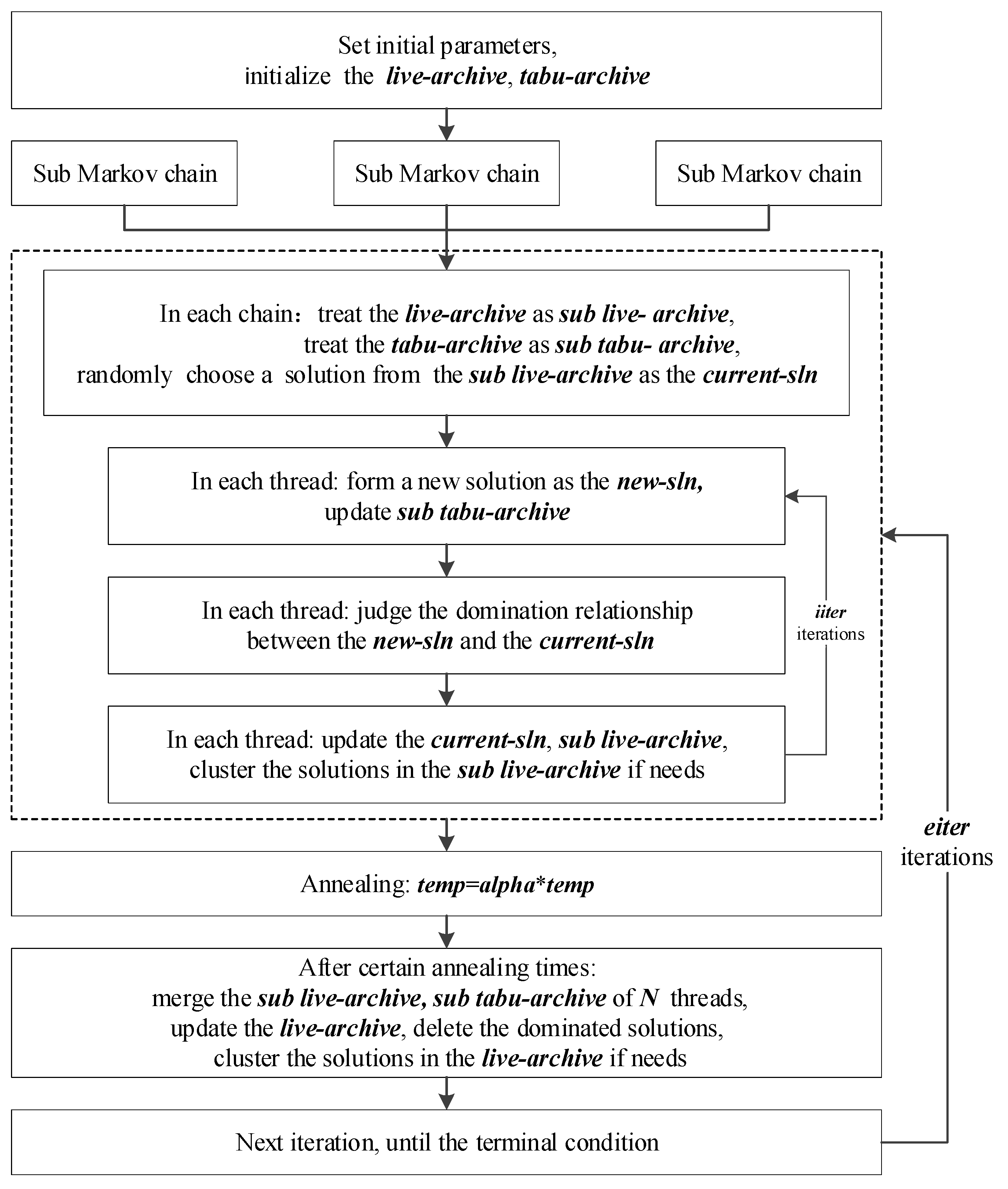
3.1. The Framework of AMOSA-II

The AMOSA-II method for spatial sampling is developed based on AMOSA. It mainly improves the optimization efficiency in terms of three aspects. First, multiple Markov chains are designed to extend the original, single Markov chain. Each one of these chains iterates independently and then shares the information after certain iterations. More chains give rise to the reinforcement of search degree and the acceleration of convergence process. The multi-core parallelization technology is introduced based on multiple Markov chains. A single Markov chain is a serialization process that is difficult to parallelize and, thus, causes limited iteration efficiency. However, parallelization becomes feasible for multiple chains and helps to further improve the iteration efficiency. In addition, a tabu-archive is designed to store the searched solutions. There is no need for any new solution that exists in the tabu-archive to be compared with the optimal solutions again, and then the computational time is saved by avoiding such repetitive and invalid comparison process.
The workflow scheme of the AMOSA-II algorithm is presented in Figure 1. The basic steps of the AMOSA-II algorithm are described below.
Step 1: Set the listed parameters: the initial temperature, Tmax; the annealing ratio, alpha; the maximum number of solutions in the live-archive that are finally returned, HL; the largest number of solutions in live-archive that triggers clustering operation, SL; the number of annealing times, eiter; the iteration number at the current temperature, iiter.
Step 2: Initialize two archives—one for storing optimal solutions, live-archive, and the other one for storing searched solutions, tabu-archive. A few initial solutions are found by using a simple hill-climbing technique; these remain nondominated to each other and then are added into the two archives.
Step 3: Create multiple Markov chains. Multiple Markov chains run in parallel based on multiple threads with the support of multi-core parallelization technology.
Step 4: In each chain, the tabu-archive is treated as the sub tabu-archive, the live-archive is treated as the sub live-archive, and one solution is selected randomly from the sublive-archive as the chain’s current solution, current-sln.
Step 5: In each chain, a new solution is generated by random perturbation of the current-sln, and its existence in the sub tabu-archive is judged. If it is not in the sub tabu-archive, then it is treated as the new solution, new-sln, and the sub tabu-archive is updated by archiving the new-sln and clustered to the HL size if its size exceeds SL. Otherwise, a new solution must be generated.
Step 6: In each chain, compare the domination relationship between the current-sln and the new-sln by the judgment rule based on AMOSA.
Step 7: In each chain, update the current-sln, sub live-archive based on the comparison output.
Step 8: The process above, from Steps 4 to 7, is repeated with iiter iterations.
Step 9: After the iiterth iteration, the current temperature tau is annealed by tau=tau*alpha.
Step 10: Repeat Steps 3 to 9, after certain annealing times, merge the sub live-archives and the sub tabu-archives in all Markov chains. The combined archive from the sub live-archives must be managed to be consisting of the solutions that are nondominated to each other and clustered to the HL size if its size exceeds SL; finally, the live-archive is updated with the processed combined archive.
Step 11: Repeat Steps 3 to 10 with eiter iterations until the terminal condition is satisfied.

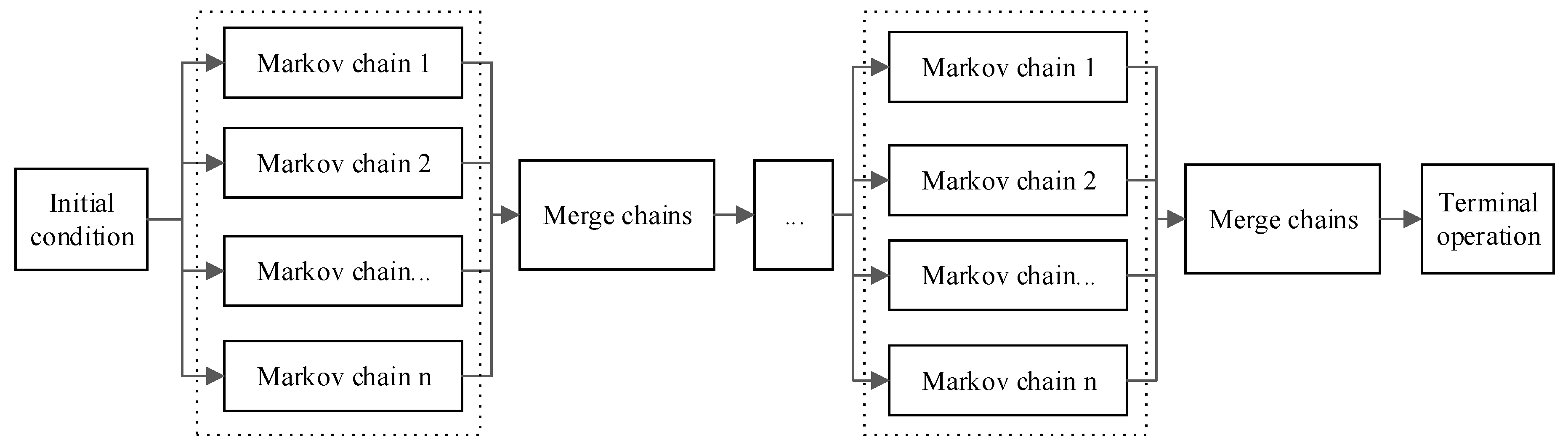
3.2. Multiple Markov Chains

Multiple Markov chains are separated from one simulated annealing chain, and they cannot only grow independently—that is, simultaneously or asynchronously—but also share information at certain moments [45]. It becomes feasible for them to parallelize with the multi-core technology in the optimization process. Multiple Markov chains obtain the optimal solutions through their own iterations, which greatly extends the search scale compared to one single Markov chain. When the combination condition is satisfied, the optimal solutions from all chains are compared, and the most optimal solutions are obtained and treated as the input of the next iteration stage for all chains. The convergence is sped up by the information interaction. Thus, optimization efficiency is improved as a result of multiple Markov chains.
In the AMOSA-II method, multiple Markov chains are designed to iterate simultaneously. The specific operation mode is presented in Figure 2. Based on the same initial condition, each Markov chain grows independently with the same frequency and gets its own nondominated solutions; thereafter, all chains are combined to extract the optimal solutions, which are treated as the inputs of the next iteration stage for each chain. The phased iteration and combination continue until the termination conditions are met.
During independent growth, for each Markov chain, the live-archive and tabu-archive are treated as the sub live-archive and sub tabu-archive, respectively. A solution is randomly selected as the current solution current-sln from the respective sub live-archive, and then the current-sln is perturbed randomly to form a new solution which is treated as the new-sln if it is not in the respective sub tabu-archive. Any newly formed solution must be added into the respective sub tabu-archive. The domination relationship between the new-sln and the current-sln is judged by the judgement rule, and then update the respective sub live-archive and the current-sln conditionally. Each chain must iterate the same frequency.
In the combination stage, each chain has its own updated sub live-archive and sub tabu-archive. All sub tabu-archives are combined, and all solutions are extracted to update the tabu-archive. The solutions from all sub live-archives are collected and compared with each other to judge the domination relationship; thereafter, the nondominated optimal solutions are then finally stored in the live-archive. Through the combination of all chains, the live-archive and tabu-archive are updated and treated as the input sub live-archive and sub tabu-archive of each chain in the next iteration stage.

3.3. Parallelization based on Multiple Markov Chains

Based on multiple Markov chains, the multi-core parallelization technology is employed in AMOSA-II to improve optimization efficiency. With the rapid development of computer science, multi-core parallelization technology has shown great computational performance [46,47]. With this technology, the main task is divided into several sub-tasks that are allocated to multiple processors as certain patterns. These processors can be the cores from the same or different computers. Then, these sub-tasks are executed independently and synchronously, the implementation process of each sub-task does not depend on those of the others. When all sub-tasks are completed, the results of all sub-tasks are collected on the basis of certain mechanisms and output as the integrated result of the main task. A single Markov chain is a serializable process that cannot be decomposed into parallel sub-tasks. For multiple Markov chains, each one iterates independently, and the iterative results must be combined after certain iterations. Therefore, the multi-core parallelization technology can be applied to multiple Markov chains, which decomposes the entire process into parallel sub-tasks to iterate synchronously with the aim of improving efficiency.
The sketch of parallelization based on multiple Markov chains is presented Figure 3. Based on a high-performance computer configured with multiple cores, the main thread first must apply for S sub-threads, and then decompose the entire iterative task based on multiple Markov chains into multiple sub-tasks. These sub-tasks are dynamically distributed to the sub-threads and each sub-thread is ensured to have one sub-task. Once one sub-task of a sub-thread is completed and then another sub-task is called in. As all sub-threads complete all sub-tasks, the results of all sub-tasks are collected by the main thread and treated as the output of the entire iterative task.
In order to attain parallelization based on multi-Markov chains, the function sfClusterApplyLB integrated in the package snowfall (provided in the R platform) is employed [48]. It only requires a few parameters—such as the size of the cores for parallelization and the functions or arguments to call—and it is not concerned with the specific parallelization operation, such as task decomposition or thread allocation. Moreover, it is exceedingly convenient for developers to learn and use. In addition, the function sfClusterApplyLB can achieve load balancing compared with other parallelization functions, which implies that when one thread completes its sub-task, it will call in the next sub-task immediately without waiting for all the other threads to complete their sub-tasks. Thus, the load balancing mode can improve computational efficiency by making full use of threads and cutting out idle time.

3.4. The Tabu-Archive Constraint

The tabu-archive constraint is designed based on the tabu search operation to avoid repeated searching solutions. As there is a possibility of searching a solution multiple times, the tabu search operation is a traditional method to avoid repeated searching in optimization [49]. In AMOSA-II, a tabu-archive with no size limit is designed to store solutions that have already been searched by all Markov chains, and it is shared by all Markov chains as their own sub tabu-archives; moreover, each sub tabu-archive is updated when forming a new solution during their own iteration process, and then all sub tabu-archives are combined during the combination stage to update the tabu-archive. During the independent iteration process, once a new solution is formed by random perturbation, it is necessary to judge whether the solution exists in the subtabu-archive of the respective chain. If archived, the newly formed solution must be ignored, and another perturbation must be performed to obtain another new solution. All the newly formed solutions of each Markov chain are added to the respective sub tabu-archive.
Due to the fact that repeatedly searching a solution leads to extra computational time without any optimization, the tabu-archive constraint is designed to help save the optimization time. In the absence of the tabu-archive constraint, solutions that have been found in previous procedures may be searched by perturbation; then, its domination relationships with other solutions in the live-archive would be judged repeatedly. However, the judging process is complex and time-consuming; moreover, it is invalid without any improvement in the convergence of the optimal solutions and, finally, this would give rise to extra computational time. On the contrary, with the tabu-archive constraint, the duplicate solution can be excluded, and the extra invalid judging process is avoided; consequently, the extra computational time is saved, and the overall optimization efficiency is improved.

3.5. Complexity Analysis

The complexity of AMOSA-II was analyzed based on the AMOSA method. As illustrated above, the AMOSA-II method has n ( n >1) Markov chains and AMOSA has only one, which is the main difference between them. The multi-core parallelization technology with m threads is applied on the basis of multiple Markov chains; then, the computational time for multiple Markov chains is the same for one Markov chain within the equal iterations at the current temperature. However, for the same stable distribution of solutions, the number of iterations at current temperature for AMOSA-II is less than that of AMOSA with the advantage of multiple chains; thus, the total number of iterations for AMOSA-II is less than that of AMOSA. The other parts of the proposed method AMOSA-II are almost the same as that of AMOSA. As illustrated by Bandyopadhyay [16], the complexity of AMOSA is expressed in the following manner.
C o m p l e x i t y = O ( T o t a l I t e r × N × ( M + log ( N ) ) )
where T o t a l I t e r stands for the total number of iterations, N is the archive size HL and M is the number of objectives.
Based on the above analysis, the complexity of AMOSA-II is expressed in the following manner.
C o m p l e x i t y = O ( T o t a l I t e r n × N × ( M + log ( N ) )

3.6. Performance Indices

A good multi-objective optimization method is expected to provide satisfied optimal solutions efficiently. The computational time is a performance index to reflect the efficiency of converging to the Pareto optimal solution set. In addition, A preeminent set of optimal solutions obtained by a multi-objective optimization method must satisfy two conditions [50]. One is that the Pareto front, consisting of optimal solutions, must be as convergent to the true Pareto front as possible. The other one is that the optimal solutions must be as diverse as possible. In order to evaluate the performance of the optimal solutions obtained by a multi-objective optimization method according to these two conditions, five performance indices have been proposed and widely accepted in the multi-objective optimization field. These are: the convergence [11], purity, spacing, min-spacing [51] and displacement [52]. The formulas and parameters’ descriptions of these six indices are listed in Table 1.
Convergence is the quantification of the convergent degree of the obtained Pareto optimal solution set to a known Pareto optimal set. The lower the value, the more approximate the obtained set to the known set. Purity is to evaluate the contribution degree of different solution sets. These solution sets are first collected to form the final optimal solution set, and then the proportion of the optimal solutions from a specific solution set, which are also part of the final optimal solution set; this is calculated to reflect its contribution degree, between 0 and 1. The higher the value, the more convergent the solution set compared to other solution sets. The spacing index can indicate the uniformity of the optimal solutions, and the min-spacing index is evolved to make up for the defect that the spacing index may yield wrong results for extreme cases, even though occasionally it may also under perform. The lower the values of these indices, the more uniform the solutions. The displacement index is used to estimate the difference between the obtained solution set and the known Pareto front. The lower the value, the better the convergence and diversity of the obtained optimal solutions.

4. Performance Test on Traditional Test Problems

4.1. Experiment Case

In order to analyze the optimization performance of AMOSA-II for multi-objective optimization problems, the experiment case is designed based on traditional test problems as the manner which is widely used by other studies [11,13,16]. There are disparate Pareto front types for different multi-objective optimization problems. The form may be convex or nonconvex, and the distribution may be continuous or discontinuous, uniform or non-uniform. On behalf of different types of Pareto front, six traditional test problems are selected to test the performance of the AMOSA-II method. These are: ZDT1, ZDT2, ZDT3, ZDT4, ZDT6 [50], and DTLZ2 [53]. Detailed information regarding the functions and the form traits of the Pareto fronts are listed in Table 2.

4.2. Experiment Design
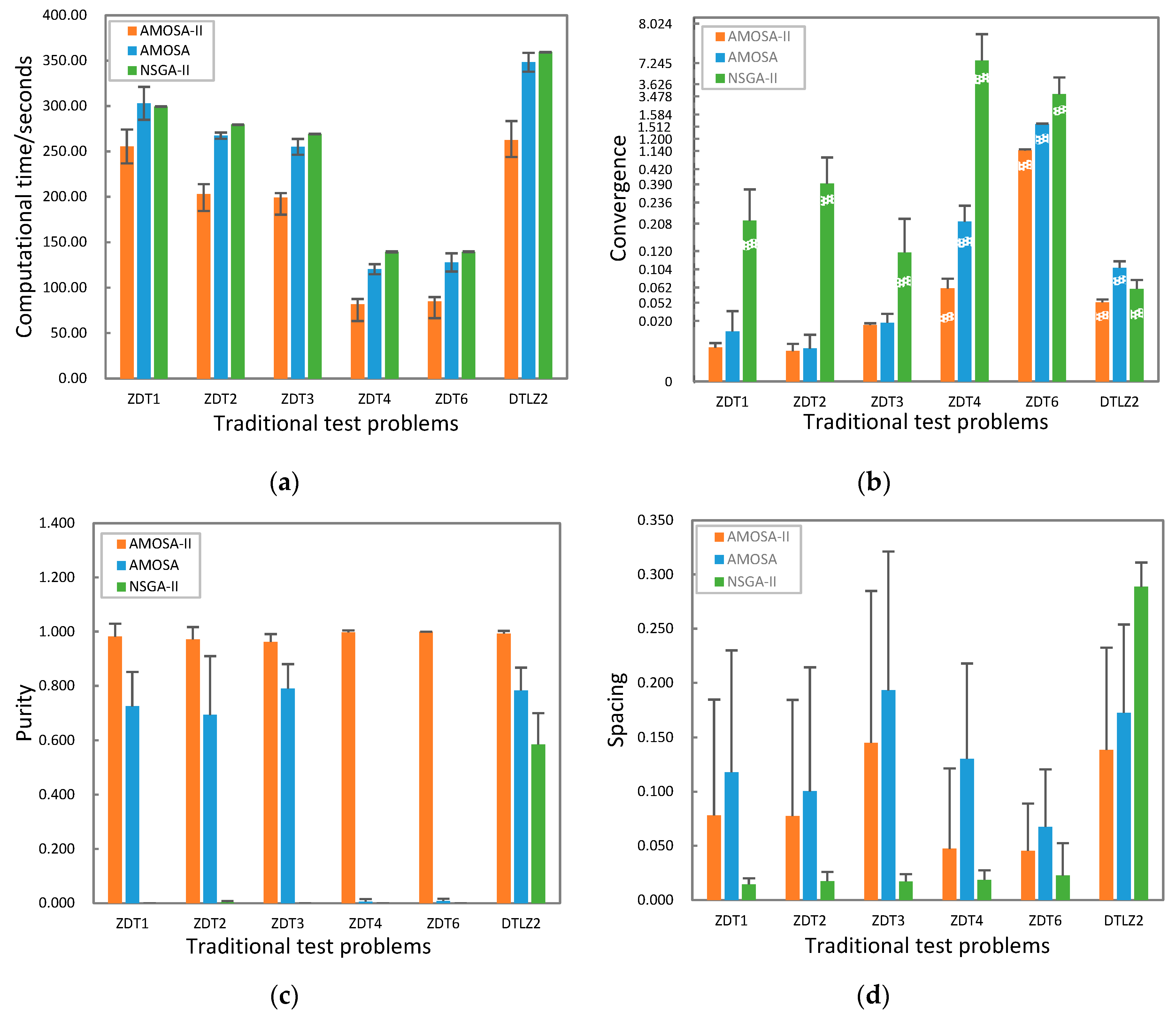
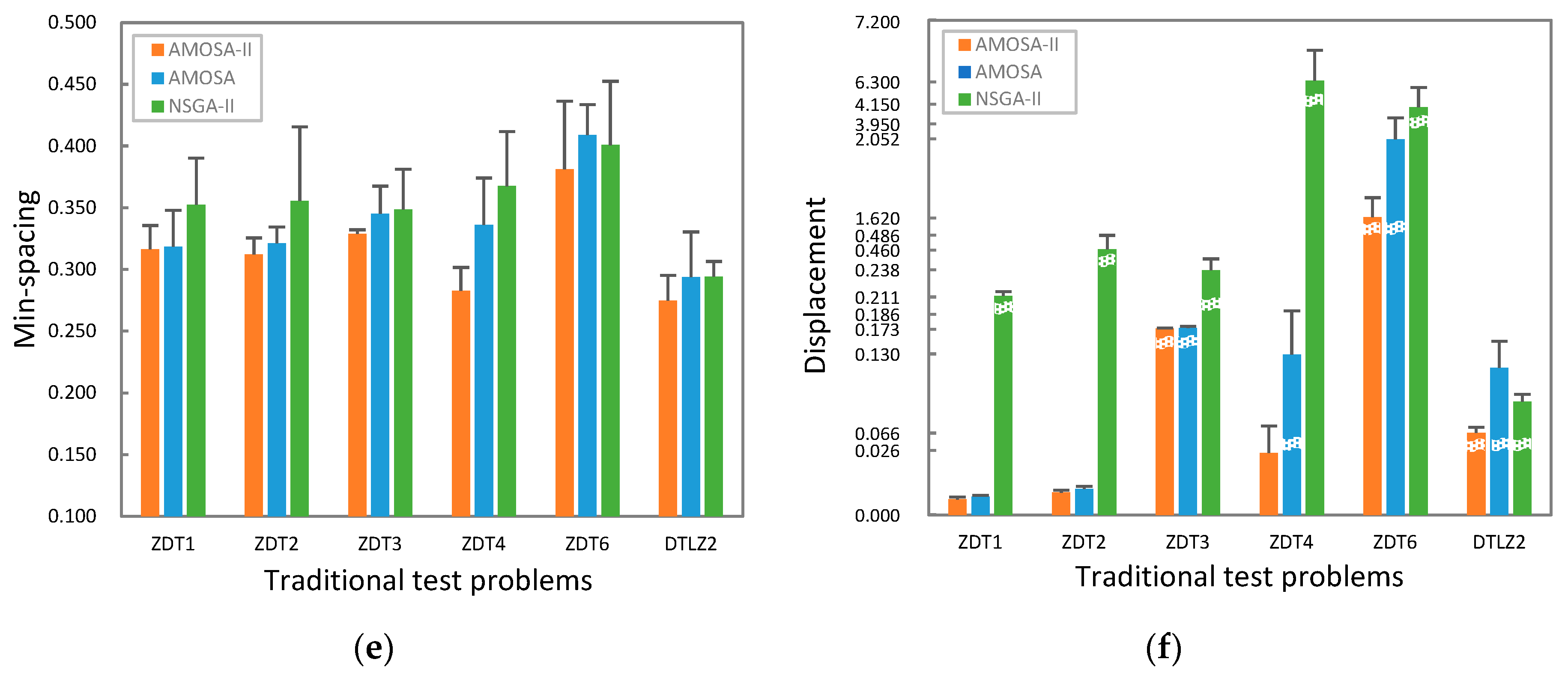
Based on the six traditional test problems, the performance of AMOSA-II is compared with its unimproved version AMOSA, and NSGA-II which is a frequently used multi-objective optimization method in other fields with high computing efficiency [54,55,56]. For all algorithms, the test problems were respectively initialized with the same sets of solutions. For the former two algorithms, the random perturbation was used to generate a new solution—the HL was 100 and SL was 110 for each problem; meanwhile, the traditional method of selection, crossover and mutation is used to obtain the offspring solutions for NSGA-II, and its solution set size was 100 for each problem. For AMOSA-II and AMOSA, the initial temperature and annealing ratio were set as the comparison experiment of the AMOSA algorithm used by Bandyopadhyay [16], which were 200 and 0.8. For NSGA-II, the crossover probability was 0.9 and the mutation probability was 1/l (l is the string length), both of which are recommended by Goldberg [57]. For AMOSA-II, there were three Markov chains, three parallelizing threads. The respective iiter for all six problems were 50, 50, 50, 20, 20, and 50, and the respective eiter were 15, 15, 15, 10, 10, and 7, the respective combination frequency were 7, 7, 7, 2, 2, and 5. For AMOSA, the iteration number for all six problems was 500. For NSGA-II, the generation numbers were 240, 240, 240, 110, 110, and 300. The true Pareto front with 200 solutions for each test problem was obtained based on the definition provided by Deb [50]. These three algorithms, related multi-objective functions, and the extraction of the solutions in the true Pareto front for six test problems were coded based on the R language. The traditional problems were tested on a PC with 128GB RAM and four processors (Inter R Xeon R CPU e7-4850, 2.20GHz, 14cores).

4.3. Results

Based on the design illustrated in the Section 4.2, experiments for AMOSA-II, AMOSA and NSGA-II were executed ten times for each test problem. The performance indices of each problem were obtained by counting the average value and standard deviation (SD) of the ten rounds.
The results of performance indices are listed in Figure 4. For all six test problems, the computational time for AMOSA-II is distinctly less than that of AMOSA and NSGA-II. The convergence of AMOSA-II is slightly greater than that of AMOSA and NSGA-II, and the purity of AMOSA-II is significantly greater than that of the other two algorithms. The two indices indicate that AMOSA-II has better convergence performance than AMOSA and NSGA-II. The spacing and min-spacing indices of AMOSA-II are lower than those of AMOSA, which signifies that AMOSA-II obtains more uniform coverage of the Pareto front as compared to AMOSA. The spacing and min-spacing indices of AMOSA-II and NASG-II tend to fluctuate, which reflects that the uniformity of the coverage of optimal solutions with the two algorithms depends on the case. The displacement of AMOSA-II is lower than that of AMOSA and NSGA-II, thereby implying that AMOSA-II can obtain better optimal solutions that are more convergent and more diverse.
In addition, the respective SD indices for each algorithm, which is represented by the error line of the bar graph in the Figure 4, is analyzed. The SD of computational time for AMOSA-II is comparable with AMOSA, but higher than NSGA-II, which implies that the computational time for AMOSA-II is not as stable as that for NSGA-II. This is partially because the number of searched optimal solutions changes in each iteration for AMOSA-II and AMOSA. Based on the varying number of solutions, the amount of judging operating is varying and the time for clustering operation is also not guaranteed to be stable. However, for NSGA-II, the number of solutions is fixed in each generation which makes it much more stable in terms of computational time. The SD indices of convergence, purity, and displacement for AMOSA-II is lower than those of AMOSA and NSGA-II, which implies that the quality of optimal solutions is more stable. The SD indices of spacing and min-spacing for three algorithms is fluctuant, which implies that the uniform distribution of optimal solutions is not stable.
Based on the results of these six indices, in comparison with AMOSA and NSGA-II, AMOSA-II obtained optimal solutions with better convergence in less time, the uniformity of AMOSA-II is better than that of AMOSA but not NSGA-II, which depends on the case. The stability of its running time is comparable with AMOSA but not as good as NSGA-II, and the quality of its optimal solutions is more stable than that of the other two.

5. Performance Analysis in Spatial Sampling

5.1. Experiment Case

In order to test the application performance of AMOSA-II for complex geographical spatial sampling optimization, the study case employed by Lark [17] for soil sampling is imported here. In this application case, the field to be sampled is square, with each side measuring 100 m; however, the part that is centered on the right corner with a 40-meter radius is missing. As Lark described, the spatial statistical quality and sampling efficiency are two key points that need to be taken into consideration in a sampling design. The spatial statistical quality can be estimated by the sample standard error which is expected to be less for better spatial coverage of the sample points; moreover, the sampling efficiency can be reflected by the total distance to all sample points which is expected to be minimized. There are tradeoffs between the spatial coverage and sampling efficiency. In general, better sampling efficiency may result in poor spatial coverage, and good spatial coverage can lead to poor sampling efficiency. Thus, the multi-objective optimization method can be applied to obtain optimal sampling designs that satisfy these two aspects.
In this case, the first objective function is the variance of the sample mean. It is optimized to achieve good spatial coverage. The spatial correlation of the soil variable in this region is assumed to be a spherical variogram whose range is 100m, nugget variance is 500 and correlated variance is 4500, Then, the variance of the sample mean is estimated based on the following formulas with the given variogram parameters [58]:
σ m 2 = 2 n i = 1 n γ ¯ ( X i , B ) 1 n 2 i = 1 n j = 1 n γ ( X i X j ) γ ¯ ( B , B )
γ ¯ ( X i , B ) = X k B o γ ( X i X k ) d X k
γ ¯ ( B , B ) = X k B 0 X l B o γ ( X k X l ) d X l d X k
where X i represents the coordinates of the i th sample site, and γ is the variogram of two sites in domain B .
The other one is the total distance to all sample points. The optimization yields the minimum total distance. The starting and leaving locations are at the bottom-left of the domain, with the coordinates (0, 0), and the shortest route to visit a set of candidate sample points is estimated based on the solve_TSP method, which is a two-edge exchange improvement procedure integrated in the TSP package by the R platform [59].

5.2. Experiment Design
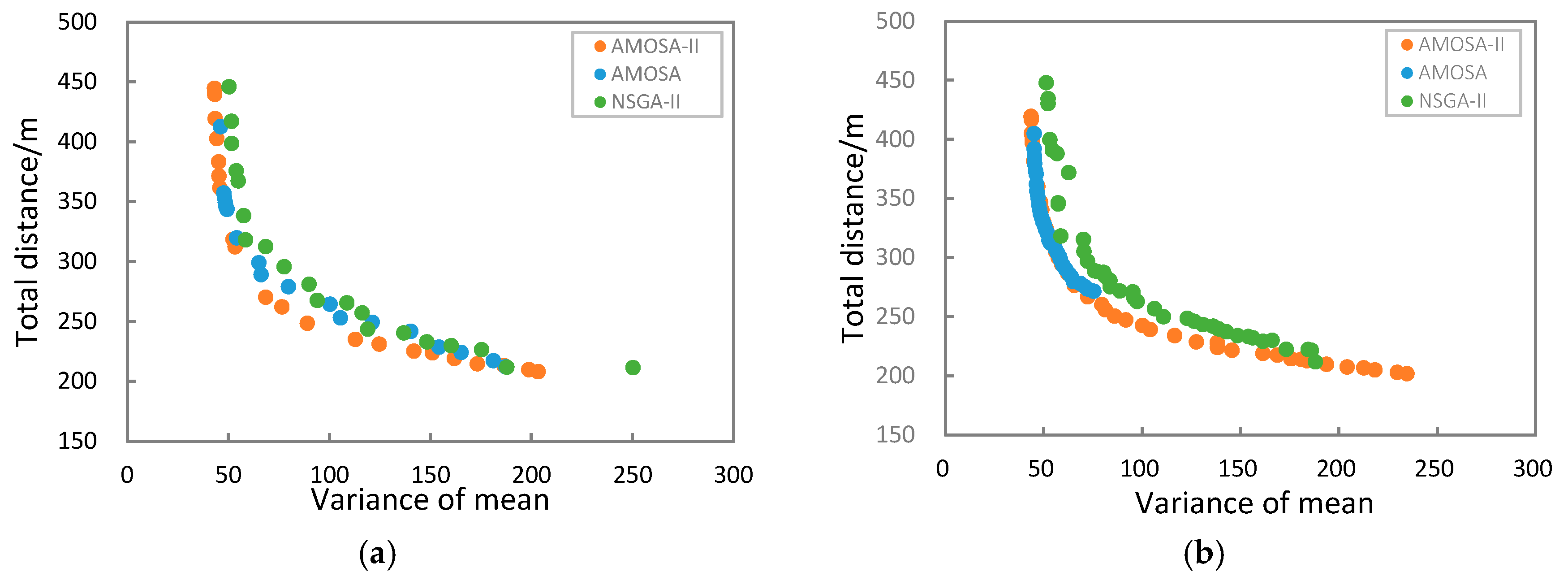
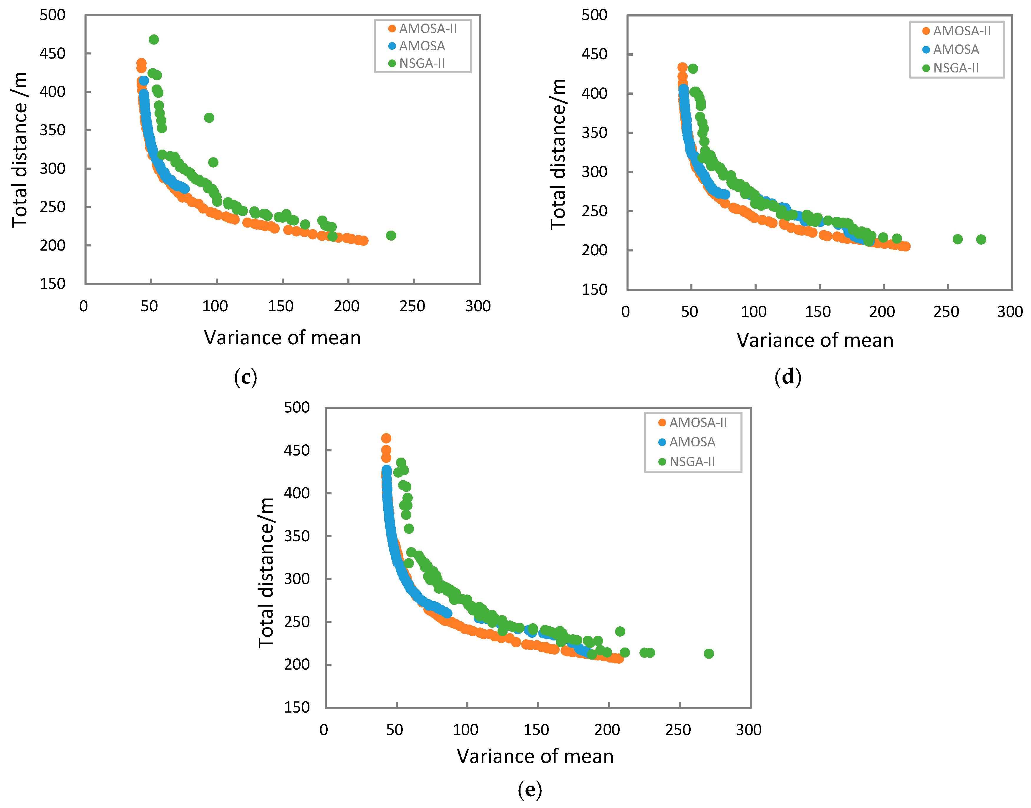
Based on the multi-objective optimization spatial sampling case, the application performance of AMOSA-II is compared with AMOSA and NSGA-II. Five experiment groups with the sample size (HL) 20, 40, 60, 80, and 100 are designed in the following manner. For all experiments with the former two algorithms, the related parameter settings in Lark’s case were shared. The sample size remained 20, the initial temperature was 1, and annealing ratio was 0.99. The SL was respectively set as 30, 50, 70, 90, and 110. For AMOSA-II, there were 20 Markov chains, and 20 parallelization threads; the combination frequency was 8 and the total iteration number was 3200 across five experiments, respectively. For AMOSA, the total iteration number was 2000. For NSGA-II, the crossover probability was 0.9, the mutation probability was 0.1, and the respective generation numbers were 8400, 5200, 3000, 2300, and 1800. The parameter settings are listed in Table 3. The code for these multi-objective functions provided in Lark’s work is employed in this paper. This experiment case was performed on a PC with 128GB RAM and four processors (Inter R Xeon R CPU e7-4850, 2.20GHz, 14cores).
In addition, related experiments were conducted to further analyze the efficiency of AMOSA-II from three aspects. Experiment A is designed for analyzing the effect of the number of Markov chains on operating efficiency, experiment B is for analyzing the effect of the number of parallelization threads on operating efficiency, and experiment C is for analyzing the effect of the combination frequency on operating efficiency. For each case, five sub experimental groups with the sample size (HL) 20, 40, 60, 80, and 100 are designed in the following manner. For all groups, the initial temperature was 1, the annealing ratio was 0.99, and the SL was respectively set as 30, 50, 70, 90, and 110. The parameters settings for experiments A, B, and C are listed in Table 4.

5.3. Results

Based on the design illustrated in Section 5.2, AMOSA-II, AMOSA and NSGA-II are applied for soil sampling optimization; the results of the performance indices are listed in Figure 5. For all optimal solution set sizes (20HL, 40HL, 60HL, 80HL, and 100HL), as depicted in Figure 5a, the computational time of AMOSA-II is approximately 223 min, and that of AMOSA is nearly 316 min, that of NSGA-II is about 330 min. The convergence time of AMOSA-II is almost 40% lower than that of AMOSA and 47% lower than that of NSGA-II. Figure 5b indicates that all the convergence indices of AMOSA-II are lower than those of AMOSA and greatly lower than those of NSGA-II. Figure 5c indicates that all the purity indices of AMOSA-II are close to 1, and the purity indices of AMOSA for the optimal solution set size with 20HL, 40HL, and 100HL are lower than 0.8 and those for 60HL, 80HL are close to 0. Moreover, the purity indices of NSGA-II for all set size are almost 0. The lower convergence indices and higher purity indices for all optimal solution set sizes illustrate that the optimal solutions obtained by AMOSA-II are much more convergent than those obtained by AMOSA and NSGA-II. As depicted in Figure 5d,e, the spacing indices of AMOSA-II with the 40HL, 80HL, and 100HL solution set sizes are higher than those of AMOSA and NSGA-II, while the min-spacing indices of AMOSA-II with the 20HL, 40HL, and 80HL solution set sizes are higher than those of AMOSA and NSGA-II. This indicates that the diversity or uniformity of these solution sets obtained by AMOSA-II is not superior to or even worse than that of AMOSA or NSGA-II. As illustrated in Figure 5f, the displacement indices of all optimal solution set sizes based on AMOSA-II are much higher than those of AMOSA and NSGA-II. This indicates that the optimal solutions generated by AMOSA-II are much more convergent and more diverse than those generated by AMOSA and NSGA-II. The results of the displacement indices are not unanimous with the results of the spacing and min-spacing indices, and this supports that idea that the spacing and min-spacing indices are not sufficiently adequate to reflect the uniformity degree of the solutions in certain cases, which are explained by Bandyopadhyay [16]. Based on the four indices of computational time, convergence, purity and displacement, for the soil sampling optimization application case, it can be inferred that AMOSA-II improved the optimization efficiency with more optimal solutions than those provided by AMOSA and NSGA-II.
Based on the optimization result obtained with AMOSA-II, AMOSA, and NSGA-II, the spreading of their optimal solutions is presented in Figure 6. The results reveal that the optimal solutions from AMOSA-II denominate more solutions than those of AMOSA and NSGA-II, which implies that the optimal solutions of AMOSA-II are more convergent. The spreading of the optimal solution set obtained with AMOSA-II is relatively more uniform, while the optimal solutions obtained with AMOSA and NSGA-II algorithms are relatively more unevenly spread. This is inconsistent with the above results of the spacing and min-spacing indices, and it further supports the argument that the two indices do not accurately describe the distribution uniformity of the solution set, which is declared by Bandyopadhyay [16]. In conclusion, the optimization of soil multi-objective sampling with AMOSA-II is improved not only for the computational efficiency, but also for the convergence and uniformity of the optimal solution set.

6. Discussion

The AMOSA-II method is developed based on the simulated annealing algorithm: the setting of initial parameters determines the implementation performance of the simulated annealing schedule. As illustrated in Section 3.1, the related key initial parameters are the maximum temperature (Tmax), annealing ratio (alpha), number of iterations (iiter) and terminal condition. The maximum temperature is treated as the initial temperature to get the entire solution space, and several methods for its selection have been recommended by Suman and Kumar [60]. The acceptance ratio is a key index that must be taken into consideration. In AMOSA-II, the initial temperature is set in the same manner as in AMOSA to obtain an initial acceptance rate of approximately 50% [16]. The annealing schedule determines the rate of temperature change. The proportional annealing schedule is used in the proposed method and the value of alpha can be set between 0.5 and 0.99 based on the need [60]. The parameter iiter indicates the number of iterations at each temperature. The determination of the iiter value must consider the actual situation [60], but the main criterion is to ensure efficient searching for the stable distribution of solutions at each temperature. The terminal condition can be set in various ways such as the minimum temperature, the number of total iterations or the value constraints of multiple objectives [60]. In AMOSA-II, the number of total iterations is recommended as the product of the number of iterations at each temperature (iiter) and the number of annealing times (eiter). Additionally, the hard and soft limit size of live-archiveHL and SL can be set depending on user needs—there is no set criterion for this.
The influence on the efficiency of AMOSA-II in terms of three aspects—the number of chains, number of parallelization threads, and combination frequency, are discussed further below.
First, the effect of the number of Markov chains on the algorithm efficiency is analyzed on the basis of experiment A. As depicted in Figure 7, the running time gradually increased from 150 min to approximately 220 min as the number of Markov chains increased, which implies that more chains increase the running time. In addition, more chains also imply more intensive search for optimal solutions, and fewer chains means possible insufficient search, which may affect the performance of optimal solutions. However, an excessive number of chains can result in extraordinary running time, which is unacceptable for providing optimal solutions within required time; thus, the number of Markov chains must be suitable in terms of the acceptable operation time and the quality of optimal solutions.
Next, the influence of different parallelization cores on algorithm efficiency is analyzed based on the experiment B. As depicted in Figure 8, with the number of cores increasing, the running time decreased from initial 900 min (5 cores) to 280 min (20 cores), and then remained stable. In this case, just 20 cores for parallelization can take full advantage of the computer with 56 cores, and there is no need to parallelize all the computer cores. On the contrary, taking up more unnecessary cores implies less cores for other tasks, wastage of computational resources, and sacrificing the efficiency of other tasks. Therefore, the number of parallelization kernels must be more than half of the computer’s configuration, which not only guarantees the running efficiency but also saves the computing space.
Moreover, the effect of different combination frequencies on algorithm efficiency is discussed based on experiment C. As illustrated in Figure 9, the running time decreased from 230 min initially to approximately 160 min after fluctuation, and then remained stable while the combination frequency increased. The result implies that a higher combination frequency leads to greater efficiency. However, an excessively high combination frequency may result in bad convergence performance of the optimal solutions, because each chain does not iterate enough times before combined, and then the convergence of obtained optimal solutions becomes insufficient. As such, the demand for the performance of optimal solutions and the acceptable running time must be considered together to set the combination frequency.
Based on the above discussion, in the practical spatial sampling application of AMOSA-II, the acceptable running time, search intensity, and computer configuration must be considered comprehensively when setting the number of Markov chains, the number of parallelization cores and the combination frequency. A computer or cluster of computers with super high computing performance is recommended if available. When running AMOSA-II with a specific computer, if the need is to emphasize saving running time while ensuring a certain degree of search intensity, then fewer Markov chains may be better. The parallelization cores can be set at almost two to three quarters of the total, and the combination frequency can be more. If the need is to emphasize search intensity while ensuring an acceptable amount of running time, then more Markov chains can be set. It is suggested that the combination frequency must not be excessive; the parallelization cores come with the same recommendation.
Although the optimization efficiency is improved, there are a few limitations for AMOSA-II. The random perturbation way is not effective enough to form new optimal solutions, because it may get invalid solutions which are much inferior to the archived ones. In addition, the outliers of optimal solutions can lead to locally optimal search which results in affecting the globally optimal search; however, certain measures are lacked for the proposed method to deal with such outliers. These limitations provide insights for the future researches, certain perturbation mechanism can be developed to form less invalid new solutions and search optimal solutions efficiently. Moreover, some strategies can be designed to obtain optimal solutions with more diverse and uniform distribution. In future spatial sampling optimization researches, the geographical spaces are usually complex and the optimization objectives are various, the proposed AMOSA-II can be treated as a feasible method for such scenarios to obtain multiple optimal sampling designs without considering weighting.

7. Conclusions

With the aim of improving computational efficiency of the optimization process for spatial sampling which usually deals with large sampling fields and complex multiple objectives, an improved parallelized multi-objective optimization method for spatial sampling, AMOSA-II, is proposed in this article. Multiple Markov chains are designed in AMOSA-II for intensive searching optimal solutions to replace the single chain that is used in AMOSA, and the optimization information of these chains is shared among them after a certain number of iterations to promote convergence. The parallelization mechanism is employed to further accelerate the iteration process. The tabu-archive constraint is designed to avoid repeated searching for saving invalid computational time. Two experimental cases are conducted to analyze the optimization performance of AMOSA-II by comparing with AMOSA and NSGA-II, respectively. The case of six typical traditional test problems received better optimal solutions within less time using AMOSA-II than those using the other two methods, which proves the improved optimization efficiency of the proposed method. In the other case, the results for soil spatial sampling optimization show that AMOSA-II has better performance which is more effective in obtaining preferable optimal sampling designs in comparison with AMOSA and NSGA-II. Finally, it is suggested that the acceptable running time, search intensity, and computer configuration must be considered comprehensively to determine the number of Markov chains, parallelization threads and combination frequency when applying AMOSA-II for multi-objective spatial sampling optimization. With the limitations of the proposed method, future research is expected to develop perturbation mechanisms to form more valid solutions and create a strategy to obtain more diverse distribution of optimal solutions. In conclusion, AMOSA-II can be considered as a feasible method to apply in other complex geographical spatial sampling optimization problems with multiple objectives.

Author Contributions

Conceptualization, Xiaolan Li and Bingbo Gao; Methodology, Xiaolan Li, Yuchun Pan; Validation, Xiaolan Li and Bingbo Gao; Writing-Original Draft Preparation, Xiaolan Li; Writing-Review & Editing, Xiaolan Li, Bingbo Gao and Zhongke Bai; Supervision, Zhongke Bai; Project Administration, Yunbing Gao; Funding Acquisition, Yunbing Gao. All authors have read and agreed to the published version of the manuscript.

Funding

This research was funded by the National key Research and Development Program of China (2017YFD0801205), and the Science and Technology Innovation Ability Construction Project of Beijing Academy of Agriculture and Forestry Sciences (KJCX20200414).

Acknowledgments

The valuable comments from anonymous reviewers are much appreciated.

Conflicts of Interest

The authors declare no conflict of interest.

References

  1. De Gruijter, J.J.; Brus, D.J.; Bierkens, M.F.P.; Knotters, M. Sampling for Natural Resource Monitoring; Springer: Berlin, Germany, 2006. [Google Scholar]
  2. Zimmerman, D.L. Optimal network design for spatial prediction, covariance parameter estimation, and empirical prediction. Environmetics 2006, 17, 635–652. [Google Scholar] [CrossRef]
  3. Heuvelink, G.B.M.; Brus, D.J.; de Gruijter, J.J. Opimization of sample configurations for digital mapping of soil properties with universal kriging. In Digital Soil Mapping. An Introductory Perspective; Lagacherie, P., Mcbratney, A.B., Voltz, M., Eds.; Elisevier: Oxford, UK, 2007; pp. 137–154. [Google Scholar]
  4. Szatmári, G.; László, P.; Takács, K.; Szabó, J.; Bakacsi, Z.; Koós, S.; Pásztor, L. Optimization of second-phase sampling for multivariate soil mapping purposes: Case study from a wine region, Hungary. Geoderma 2018, 352, 373–384. [Google Scholar] [CrossRef]
  5. Vašát, R.; Heuvelink, G.B.M.; Borůvka, L. Sampling design optimization for multivariate soil mapping. Geoderma 2010, 155, 147–153. [Google Scholar] [CrossRef]
  6. Ballari, D.; de Bruin, S.; Bregt, A.K. Value of information and mobility constraints for sampling with mobile sensors. Comput. Geosci. 2012, 49, 102–111. [Google Scholar]
  7. Zhu, Z.; Stein, M.L. Spatial sampling design for prediction with estimated parameters. J. Agric. Biol. Environ. Stat. 2006, 11, 24–44. [Google Scholar] [CrossRef] [Green Version]
  8. Brus, D.J.; Heuvelink, G.B.M. Optimization of sample patterns for universal kriging of environmental variables. Geoderma 2007, 138, 86–95. [Google Scholar] [CrossRef]
  9. Carlos, M.F.; Peter, J.F. An overview of evolutionary algorithms in multiobjective optimization. Evol. Comput. 1995, 3, 1–16. [Google Scholar]
  10. Srinivas, N.; Deb, K. Multiobjective optimization using nondominated sorting in genetic algorithms. Evol. Comput. 1995, 2, 221–248. [Google Scholar] [CrossRef]
  11. Deb, K.; Pratap, A.; Agarwal, S.; Meyarivan, T. A fast and elitist multiobjective genetic algorithm: NSGA-II. IEEE Trans. Evol. Comput. 2002, 6, 182–197. [Google Scholar] [CrossRef] [Green Version]
  12. Joshua, D.K.; David, W.C. Approximating the nondominated front using the Pareto archived evolution strategy. Evol. Comput. 2000, 8, 149–172. [Google Scholar]
  13. David, C.; Nick, R.J.; Joshua, D.K.; Martin, J.O. PESA-II: Region-based selection in evolutionary multiobjective. In Proceedings of the Genetic and Evolutionary Computation Conference (GECCO-2001), San Francisco, CA, USA, 7–11 July 2001; pp. 283–290. [Google Scholar]
  14. Suman, B. Multiobjective simulated annealing-a metaheuristic technique for multiobjective optimization of a constrained problem. Found. Comput. Decis. Sci. 2002, 27, 171–191. [Google Scholar]
  15. Suman, B. Study of simulated annealing based algorithms for multiobjective optimization of a constrained problem. Comput. Chem. Eng. 2004, 28, 1849–1871. [Google Scholar]
  16. Bandyopadhyay, S.; Saha, S.; Maulik, U.; Deb, K. A simulated annealing-based multiobjective optimization algorithm: AMOSA. IEEE Trans. Evol. Comput. 2008, 12, 269–283. [Google Scholar] [CrossRef] [Green Version]
  17. Lark, R.M. Multi-objective optimization of spatial sampling. Spat. Stat. 2016, 18, 412–430. [Google Scholar] [CrossRef]
  18. Cheng, C.X.; Shi, P.J.; Song, C.Q.; Gao, J.B. Geographic big-data: A new opportunity for geography complexity study. Acta Geogr. Sin. 2018, 73, 1397–1406. [Google Scholar]
  19. Shen, S.; Ye, S.J.; Cheng, C.X.; Song, C.Q.; Gao, J.B.; Yang, J.; Ning, L.X.; Su, K.; Zhang, T. Persistence and Corresponding Time Scales of Soil Moisture Dynamics During Summer in the Babao River Basin, Northwest China. J. Geophys. Res. Atmos. 2018, 123, 8936–8948. [Google Scholar] [CrossRef]
  20. Zhang, T.; Shen, S.; Cheng, C.X.; Song, C.Q.; Ye, S.J. Long-range correlation analysis of soil temperature and moisture on A’rou Hillsides, Babao River Basin. Atmospheres 2018, 123, 12606–12620. [Google Scholar] [CrossRef]
  21. Burgess, T.M.; Webster, R.; Mcbratney, A.B. Optimal interpolation and isarithmic mapping of soil properties: IV. Sample strategy. Eur. J. Soil Sci. 1981, 32, 643–659. [Google Scholar] [CrossRef]
  22. Mcbratney, A.B.; Webster, R.; Burgess, T.M. The design of optimal sampling schemes for local estimation and mapping of regionalized variables.1. Theory and method. Comput. Geosci. 1981, 7, 331–334. [Google Scholar]
  23. Juang, K.; Liao, W.; Liu, T.; Tsui, L.; Lee, D. Additional sampling based on regulation threshold and kriging variance to reduce the probability of false delineation in a contaminated site. Sci. Total Environ. 2008, 389, 20–28. [Google Scholar] [CrossRef]
  24. Meirvenne, M.V.; Goovaerts, P. Evaluating the probability of exceeding a site-specific soil cadmium contamination threshold. Geoderma 2001, 102, 75–100. [Google Scholar] [CrossRef]
  25. Hengl, T.; David, G.R.; Stein, A. Soil sampling strategies for spatial prediction by correlation with auxiliary. Aust. J. Soil Res. 2003, 41, 1403–1422. [Google Scholar] [CrossRef]
  26. Gao, B.B.; Pan, Y.C.; Chen, Z.Y.; Wu, F.; Ren, X.H.; Hu, M.G. A spatial conditioned latin hypercube sampling method for mapping using ancillary data. Trans. GIS 2016, 20, 735–754. [Google Scholar] [CrossRef] [Green Version]
  27. Lin, Y.P.; Chu, H.J.; Huang, Y.L.; Tang, C.H.; Rouhani, S. Monitoring and identification of spatiotemporal landscape changes in multiple remote sensing images by using a stratified conditional Latin hypercube sampling approach and geostatistical simulation. Environ. Monit. Assess. 2011, 177, 353–373. [Google Scholar] [CrossRef]
  28. Ge, Y.; Wang, J.H.; Heuvelink, G.B.M.; Jin, R.; Li, X.; Wang, J.F. Sampling design optimization of a wireless sensor network for monitoring ecohydrological processes in the Babao River basin, China. Int. J. Geogr. Inf. Sci. 2014, 29, 92–110. [Google Scholar] [CrossRef]
  29. Van Groenigen, J.W.; Stein, A. Constrained optimization of spatial sampling using continuous simulated annealing. J. Environ. Qual. 1998, 27, 1078–1086. [Google Scholar] [CrossRef]
  30. Van Groenigen, J.W.; Siderius, W.; Stein, A. Constrained optimisation of soil sampling for minimisation of the kriging variance. Geoderma 1999, 87, 239–259. [Google Scholar] [CrossRef]
  31. Van Groenigen, J.W. The influence of variogram parameters on optimal sampling schemes for mapping by kriging. Geoderma 2000, 97, 223–236. [Google Scholar] [CrossRef]
  32. Richard, W.; Murray, L. Filed Sampling for Environmental Science and Management; Routledge: Oxon, UK, 2013. [Google Scholar]
  33. Wadoux, A.; Brus, D.J.; Heuvelink, G.B.M. Sampling design optimization for soil mapping with random forest. Geoderma 2019, 355, 11. [Google Scholar] [CrossRef]
  34. Tavakoli-Someh, S.; Rezvani, M.H. Multi-objective virtual network function placement using NSGA-II meta-heuristic approach. J. Supercomput. 2019, 75, 6451–6487. [Google Scholar] [CrossRef]
  35. Xue, Y. Mobile robot path planning with a non-dominated sorting genetic algorithm. Appl. Sci. Basel 2018, 8, 2253. [Google Scholar] [CrossRef] [Green Version]
  36. Rayat, F.; Musavi, M.; Bozorgi-Amiri, A. Bi-objective reliable location-inventory-routing problem with partial backordering under disruption risks: A modified AMOSA approach. Appl. Soft Comput. 2017, 59, 622–643. [Google Scholar] [CrossRef]
  37. Memari, A.; Rahim, A.R.A.; Hassan, A.; Ahmad, R. A tuned NSGA-II to optimize the total cost and service level for a just-in-time distribution network. Neural Comput. Appl. 2017, 28, 3413–3427. [Google Scholar]
  38. Rabiee, M.; Zandieh, M.; Ramezani, P. Bi-objective partial flexible job shop scheduling problem: NSGA-II, NRGA, MOGA and PAES approaches. Int. J. Prod. Res. 2012, 50, 7327–7342. [Google Scholar] [CrossRef]
  39. Kaveh, A.; Moghanni, R.M.; Javadi, S.M. Ground motion record selection using multi-objective optimization algorithms: A comparative study. Period. Polytech. Civ. Eng. 2019, 63, 812–822. [Google Scholar] [CrossRef] [Green Version]
  40. Saadatpour, M.; Afshar, A.; Khoshkam, H. Multi-objective multi-pollutant waste load allocation model for rivers using coupled archived simulated annealing algorithm with QUAL2Kw. J. Hydroinform. 2019, 21, 397–410. [Google Scholar] [CrossRef]
  41. An, H.; Green, D.; Johrendt, J.; Smith, L. Multi-objective optimization of loading path design in multi-stage tube forming using MOGA. Int. J. Mater. Form. 2013, 6, 125–135. [Google Scholar] [CrossRef]
  42. Arora, R.; Kaushik, S.C.; Arora, R. Multi-objective and multi-parameter optimization of two-stage thermoelectric generator in electrically series and parallel configurations through NSGA-II. Energy 2015, 91, 242–254. [Google Scholar] [CrossRef]
  43. Pang, J.; Zhou, H.; Tsai, Y.-C.; Chou, F.-D. A scatter simulated annealing algorithm for the bi-objective scheduling problem for the wet station of semiconductor manufacturing. Comput. Ind. Eng. 2018, 123, 54–66. [Google Scholar]
  44. 44. Daniel, P.; Christoph, B.; Martin, K.; Marta, G.; Menéndez, M.; Sainz-Palmero, G.I.; Bertrand, C.M.; Klawonn, F.; Benitez, J.M. Multiobjective optimization for railway maintenance plans. J. Comput. Civ. Eng. 2018, 32, 1–11. [Google Scholar]
  45. Chandy, J.A.; Sungho, K.; Ramkumar, B.; Parkes, S.; Banerjee, P. An evaluation of parallel simulated annealing strategies with application to standard cell placement. IEEE Trans. Comput. Aided Des. Integr. Circuits Syst. 1997, 16, 398–410. [Google Scholar] [CrossRef] [Green Version]
  46. Borin, E.; Devloo, P.R.B.; Vieira, G.S.; Shauer, N. Accelerating engineering software on modern multi-core processors. Adv. Eng. Softw. 2015, 84, 77–84. [Google Scholar] [CrossRef]
  47. Ray, R.; Gurung, A.; Das, B.; Bartocci, E.; Bogomolov, S.; Grosu, R. XSpeed: Accelerating reachability analysis on multi-core processors. In Hardware and Software: Verification and Testing. HVC 2015. Lecture Notes in Computer Science; Springer: Cham, Switzerland, 2015. [Google Scholar]
  48. Mannuel, J.A.E.; Jochen, K.; Christine, P.; Markus, S.; Esmeralda, V. Hands-on tutorial for parallel computing with R. Comput. Stat. 2011, 26, 219–239. [Google Scholar]
  49. Glover, F.; Taillard, E. A Users Guide to Tabu Search. Ann. Oper. Res. 1993, 41, 1–28. [Google Scholar] [CrossRef]
  50. Deb, K. Multi-objective_optimization Using Evolutionary Algorithms; Wiley: Wiltshire, UK, 2001. [Google Scholar]
  51. Sanghamitra, B.; Pal, S.K.; Aruna, B. Multiobjective GAs, quantitative indices, and pattern classification. IEEE Trans. Syst. Man Cybern. Part B Cybern. 2004, 34, 2088–2099. [Google Scholar]
  52. Sanghamitra, B.; Sriparna, S. Unsupervised Classification: Similarity Measures, Classical and Metaheuristic Approaches, and Applications; Springer: Berlin, Germany, 2013. [Google Scholar]
  53. Deb, K.; Thiele, L.; Laumanns, M.; Zitzler, E. Scalable Multi-Objective Optimization Test Problems. In Proceedings of the 2002 Congress on Evolutionary Computation. CEC’02 (Cat. No.02TH8600), Honolulu, HI, USA, 12–17 May 2002; pp. 825–830. [Google Scholar]
  54. Turkson, R.F.; Yan, F.; Ali, M.K.A.; Liu, B.; Hu, J. Modeling and multi-objective optimization of engine performance and hydrocarbon emissions via the use of a computer aided engineering code and the NSGA-II genetic algorithm. Sustainability 2016, 8, 72. [Google Scholar] [CrossRef] [Green Version]
  55. Arshad, M.H.; Abido, M.A.; Salem, A.; Elsayed, A.H. Weighting factors optimization of model predictive torque control of induction motor using NSGA-II With TOPSIS decision making. IEEE Access 2019, 7, 177595–177606. [Google Scholar] [CrossRef]
  56. Bandyopadhyay, S.; Pal, S.K. Classification and Learning Using Genetic Algorithms Applications in Bioinformatics and Web Intelligence; Springer: Heidelberg/Berlin, Germany, 2007. [Google Scholar]
  57. Goldberg, D.E. Genetic Algorithms in Search, Opimization and Machine Learning; Addison-Wesley: New York, NY, USA, 1989. [Google Scholar]
  58. Webster, R.; Oliver, M.A. Statistical Methods in Soil and Land Resource Survey; Oxford University: Oxford, UK, 1991; Volume 86, pp. 1149–1150. [Google Scholar]
  59. Michael, H.; Kurt, H. TSP-Infrastructure for the traveling salesperson problem. J. Stat. Softw. 2007, 23. [Google Scholar]
  60. Suman, B.; Kumar, P. A survey of simulated annealing as a tool for single and multiobjective optimization. J. Oper. Res. Soc. 2006, 57, 1143–1160. [Google Scholar] [CrossRef]
Figure 1. The workflow scheme of the archived multi-objective simulated annealing (AMOSA)-II algorithm.
Ijgi 09 00236 g001
Figure 2. Scheme of multiple Markov chains.
Ijgi 09 00236 g002
Figure 3. Parallelization based on multiple Markov chains.
Ijgi 09 00236 g003
Figure 4. Performance indices of AMOSA-II, AMOSA, and NSGA-II with traditional test problems (ZDT1, ZDT2, ZDT3, ZDT4, ZDT6, and DTLZ2): (a) computational time; (b) convergence; (c) purity; (d) spacing; (e) min-spacing; (f) displacement.
Ijgi 09 00236 g004aIjgi 09 00236 g004b
Figure 5. Performance indices of AMOSA-II, AMOSA, and NSGA-II with the optimal solution set size (20HL, 40HL, 60HL, 80HL, and 100HL): (a) computational time; (b) convergence; (c) purity; (d) spacing; (e) min-spacing; (f) displacement.
Ijgi 09 00236 g005aIjgi 09 00236 g005b
Figure 6. The distribution of optimal solutions based on AMOSA-II, AMOSA, and NSGA-II with different optimal solution sizes:(a) 20HL; (b) 40HL; (c) 60HL; (d) 80HL; (e) 100HL.
Ijgi 09 00236 g006aIjgi 09 00236 g006b
Figure 7. The computational time based on different numbers of Markov chains.
Ijgi 09 00236 g007
Figure 8. The computational time based on different numbers of parallelization cores.
Ijgi 09 00236 g008
Figure 9. The computational time based on different combination frequencies.
Ijgi 09 00236 g009
Table 1. Performance indices.
Performance IndicesFormulaParameters’ Description
Computational time t = T e n d T s t a r t T s t a r t is the beginning time, T e n d is the terminating time.
Convergence [11] C = i = 1 N ( m i n { D i s ( R i , R * ) } ) / N
i = 1 , 2 , , N
N is the number of solutions in the set R ,
R i is the i th solution in the set R,
R * is the true Pareto front,
D i s ( R i , R * ) is the Euclidean distance of the R i solution from the true Pareto front R * .
Purity [51] P = r h * r h
r h = | { γ | γ ϵ S h } |
r h * = | { γ | γ ϵ S h   a n d   γ ϵ S * } |
h = 1 , 2 , , H
H is the number of algorithms used to obtain optimal solutions;
h is the h th algorithm;
γ is the solution listed in the set;
S h is the solution set obtained based on the h th algorithm;
S * is the solution set obtained based on the all algorithms by combining all solutions of all sets and retaining the nondominated solutions;
r h is the number of solutions in the set S h obtained based on the h th algorithm;
r h * is the number of solutions which not only in the set R 1 * but also in the set S * .
Spacing [51] S = 1 | Q | i = 1 | Q | ( d i d ) 2
d i = m i n { m = 1 M | f m i f m k | }
i = 1 , 2 , , Q
   k = 1 , 2 , , Q a n d k i
m = 1 , 2 , , M
i ,   k is the i th and k th solution in the obtained optimal solution set;
Q is the number of solutions in the obtained optimal solution set;
M is the number of objectives,
m is the m th of objectives;
f m i , f m k are the normalized values that indicate the m th objective values of the i th and k th solution in the optimal solution set,
d i is the sequence of the values that are the minimum sums of the absolute values of the difference between the respective objective normalized values of the i th and that of the other solutions in the set;
d is the mean value of all the d i .
Min-spacing [51] S m = 1 | Q 1 | i = 1 | Q 1 | ( d i * d * ) 2
d i * = m i n { d 1 , d 2 , , d Q }
d i = m i n { m = 1 M | f m s e q i h + 1 f m s e q i h | }
s e q i = { s i 1 , s i 2 , , s i Q }
i = 1 , 2 , , Q
h = 1 , 2 , , Q 1
m = 1 , 2 , , M
i is the i th solution in the obtained optimal solution set;
h is the h th solution ranked in the s e q i sequence;
s e q i is such a sequence of solutions: the i t h solution is treated as the seed s i 1 and marked; the unmarked solution is identified in the obtained optimal solution set that has the minimum distance to the seed and then the found solution is treated as seed s i 2 and marked. Repeat the process until all unmarked solutions are treated as seed once; such a solution sequence is called the sequence of the i th solution;
M is the number of objectives;
m is the m th of objectives;
f m s e q i h and f m s e q i h + 1 are the normalized values which indicate the m th objective values of the h th and ( h + 1 ) th solution in the s e q i sequence;
d i is the sequence of the values which are the minimum sums of the absolute values of the difference between the respective objective normalized values of the h th and ( h + 1 ) th solution in the s e q i sequence;
d i * is the corresponding sequence that has the minimum sum;
d * is the mean value of all the d i *
Displacement [52] D = 1 | P * | i = 1 | P * | ( m i n j = 1 | Q | d ( i , j ) )
i = 1 , 2 , , P *
j = 1 , 2 , , Q
i is the i th solution in the true Pareto front,
j is the j th solution in the obtained optimal solution set,
P * is the number of solutions in the true Pareto front,
Q is the number of solutions in the obtained optimal solution set,
d ( i , j ) is the Euclidean distance between the i th solution in the true Pareto front and j th solution of the obtained optimal solution set.
Table 2. The traditional test problems.
Test ProblemObjective FunctionsPareto FrontPareto Front Traits
ZDT1 [50]Two objective functions:
M i n : { f 1 ( x ) = x 1 f 2 ( x ) = g ( x ) h ( f 1 ( x ) , g ( x ) )
g ( x ) = 1 + 9 n 1 i = 2 n x i
h ( f 1 , g ) = 1 f 1 / g
n = 30 , 0 x 1 , x 2 , , x i , , x 30 1
Ijgi 09 00236 i001Convex, continuous, uniform
ZDT2 [50]Two objective functions:
M i n : { f 1 ( x ) = x 1 f 2 ( x ) = g ( x ) h ( f 1 ( x ) , g ( x ) )
g ( x ) = 1 + 9 n 1 i = 2 n x i
h ( f 1 , g ) = 1 ( f 1 / g ) 2
n = 30 , 0 x 1 , x 2 , , x i , , x 30 1
Ijgi 09 00236 i002Nonconvex, continuous, uniform
ZDT3 [50]Two objective functions:
M i n : { f 1 ( x ) = x 1 f 2 ( x ) = g ( x ) h ( f 1 ( x ) , g ( x ) )
g ( x ) = 1 + 9 n 1 i = 2 n x i
h ( f 1 , g ) = 1 f 1 / g ( f 1 / g ) s i n ( 10 π f 1 )
n = 30 , 0 x 1 , x 2 , , x i , , x 30 1
Ijgi 09 00236 i003Nonconvex, discontinuous
ZDT4 [50]Two objective functions:
M i n : { f 1 ( x ) = x 1 f 2 ( x ) = g ( x ) h ( f 1 ( x ) , g ( x ) )
g ( x ) = 1 + 10 ( n 1 ) + 2 n ( x i 2 10 c o s ( 4 π x i ) )
h ( f 1 , g ) = 1 f 1 / g
n = 10 , 0 x 1 1 , 5 x 2 , , x i , , x 10 5
Ijgi 09 00236 i004Convex
ZDT6 [50]Two objective functions:
M i n : { f 1 ( x ) = 1 exp ( 4 x 1 ) s i n 6 ( 6 π x 1 ) f 2 ( x ) = g ( x ) h ( f 1 ( x ) , g ( x ) )
g ( x ) = 1 + 9 [ ( i = 2 n x i ) / 9 ] 0.25
h ( f 1 , g ) = 1 ( f 1 / g ) 2
n = 10 , 0 x 1 , x 2 , , x i , , x 10 1
Ijgi 09 00236 i005Nonconvex, non-uniform
DTLZ2 [53]Three objective functions:
M i n : { f 1 ( x ) = ( 1 + g ( x ) ) c o s ( x 1 π / 2 ) c o s ( x 2 π / 2 ) f 2 ( x ) = ( 1 + g ( x ) ) cos ( x 1 π / 2 ) sin ( x 2 π / 2 ) f 3 ( x ) = ( 1 + g ( x ) ) sin ( x 1 π / 2 )
g ( x ) = i = 3 n ( x i 0.5 ) 2
n = 30 , 0 x 1 , x 2 , , x i , , x 30 1
Ijgi 09 00236 i006Convex
Table 3. The parameter settings of AMOSA-II, AMOSA and NSGA-II.
ParametersAMOSA-IIAMOSANSGA-II
Sample points202020
Markov chains 2011
Parallelization threads2011
Combination frequency800
Table 4. The parameter settings for Experiments A, B, and C.
ItemParametersValue
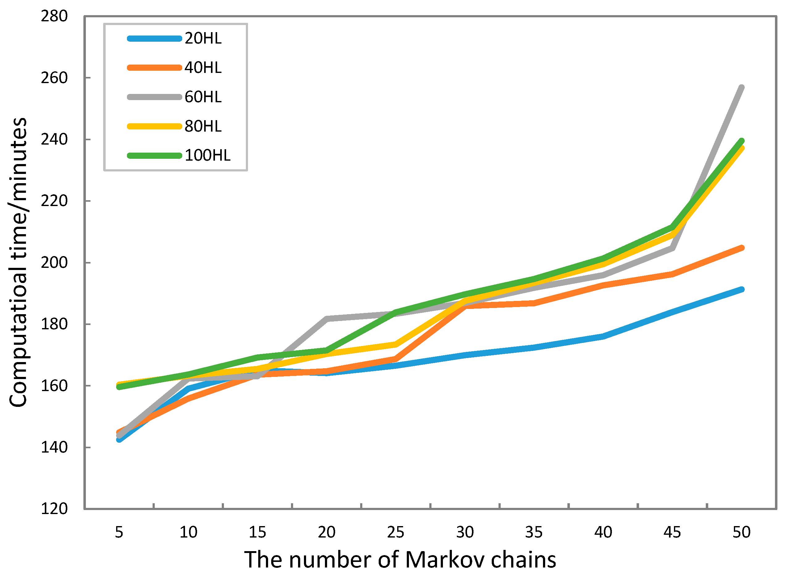
Experiment A.
The effect of the number of Markov chains on operating efficiency
Sample points20
Markov chains5, 10, 15, 20, 25, 30, 35, 40, 45, 50
Parallelization threads50
Combination frequency8
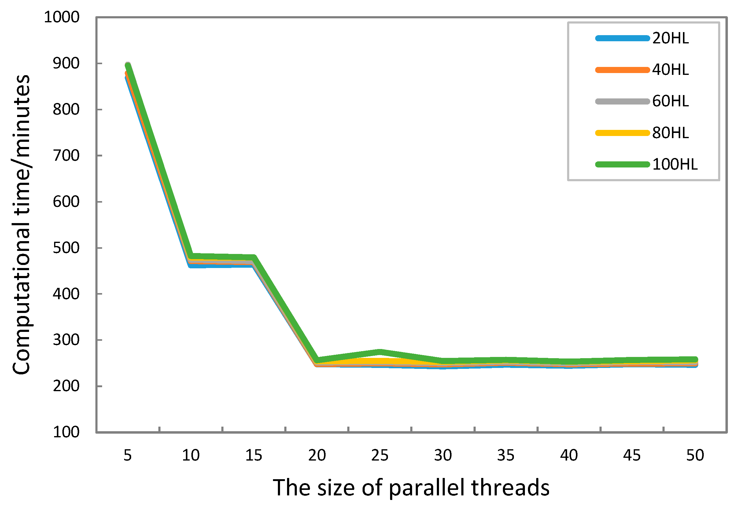
Experiment B.
The effect of the number of parallelization threads on operating efficiency
Sample points20
Markov chains20
Parallelization threads5, 10, 15, 20, 25, 30, 35, 40, 45, 50
Combination frequency8
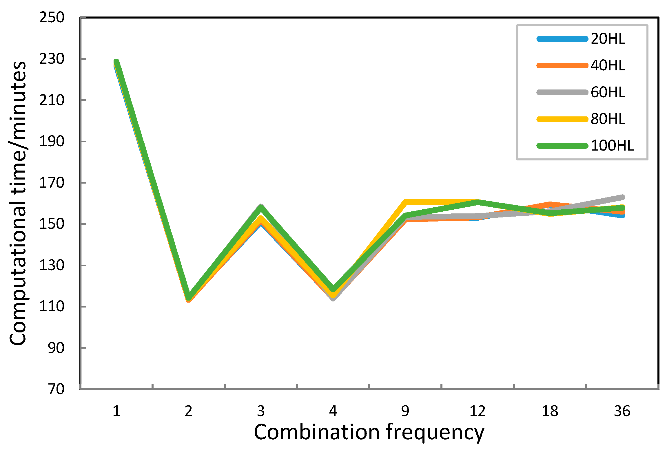
Experiment C.
The effect of combination frequency on operating efficiency
Sample points20
Markov chains20
Parallelization threads20
Combination frequency1, 2, 3, 4, 9, 12, 18, 36

