Identifying Urban Residents’ Activity Space at Multiple Geographic Scales Using Mobile Phone Data


Abstract
:1. Introduction
2. Study Area and Datasets
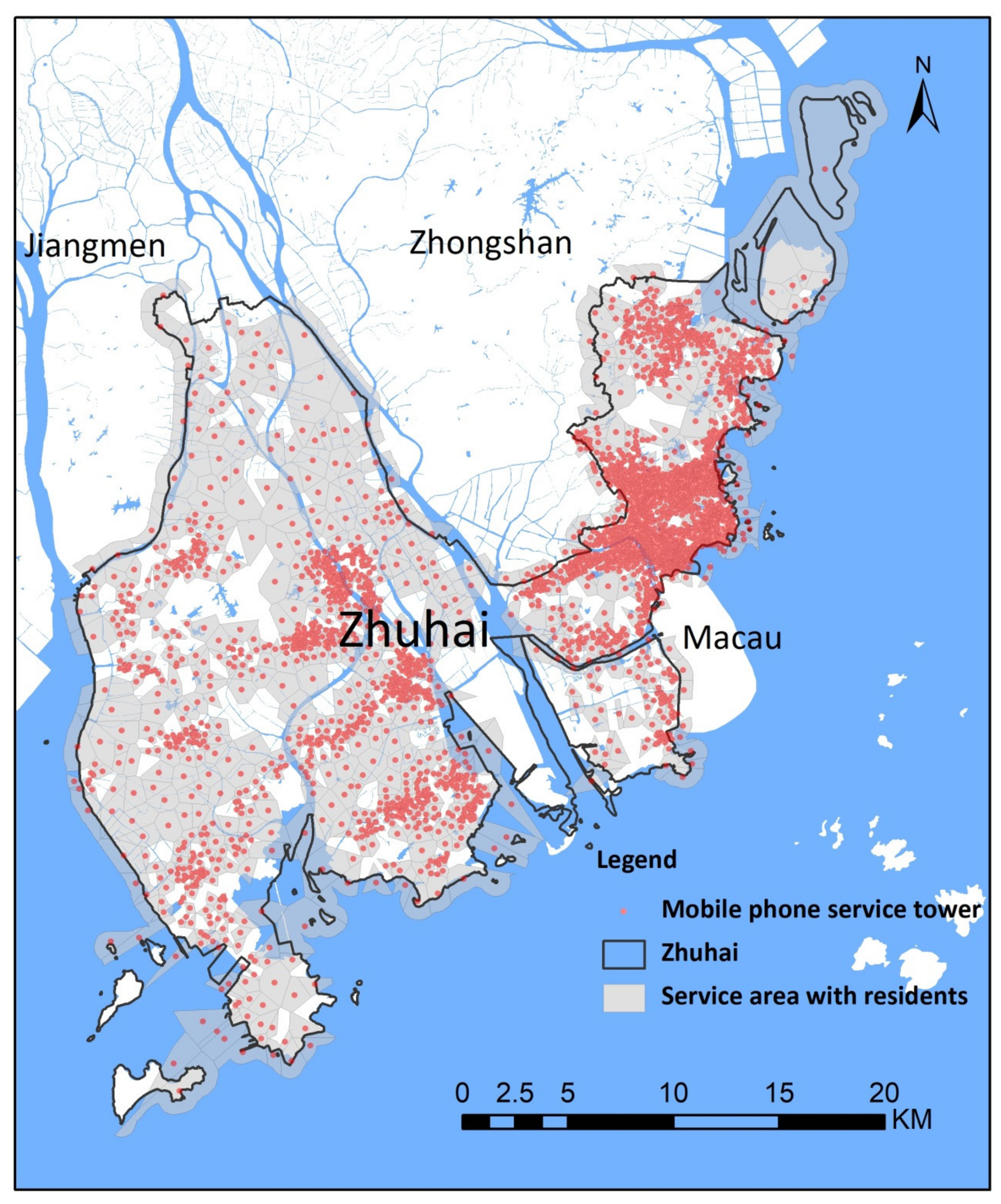
2.1. Study Area
2.2. Datasets
3. Methodology
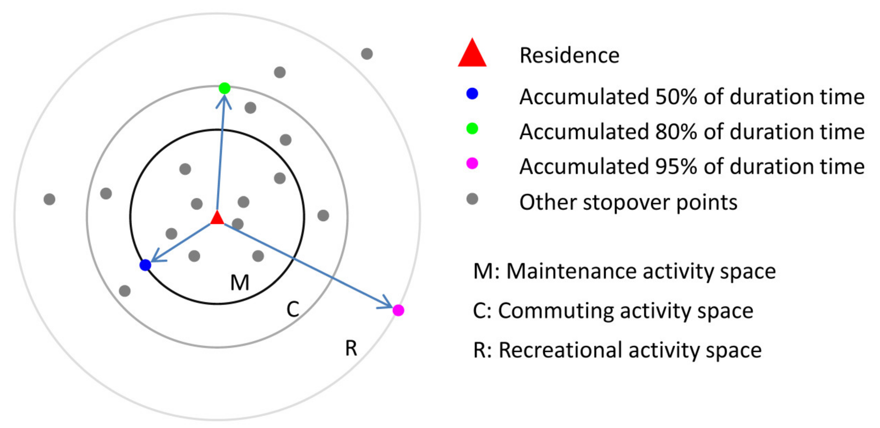
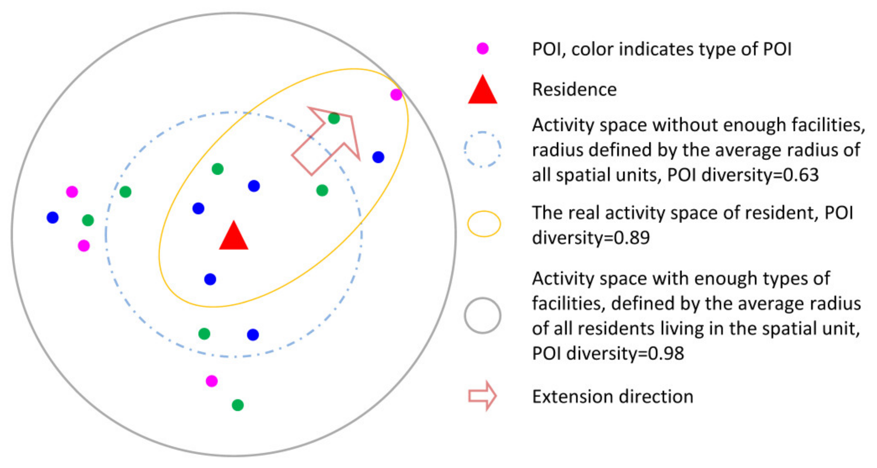
3.1. Activity Space
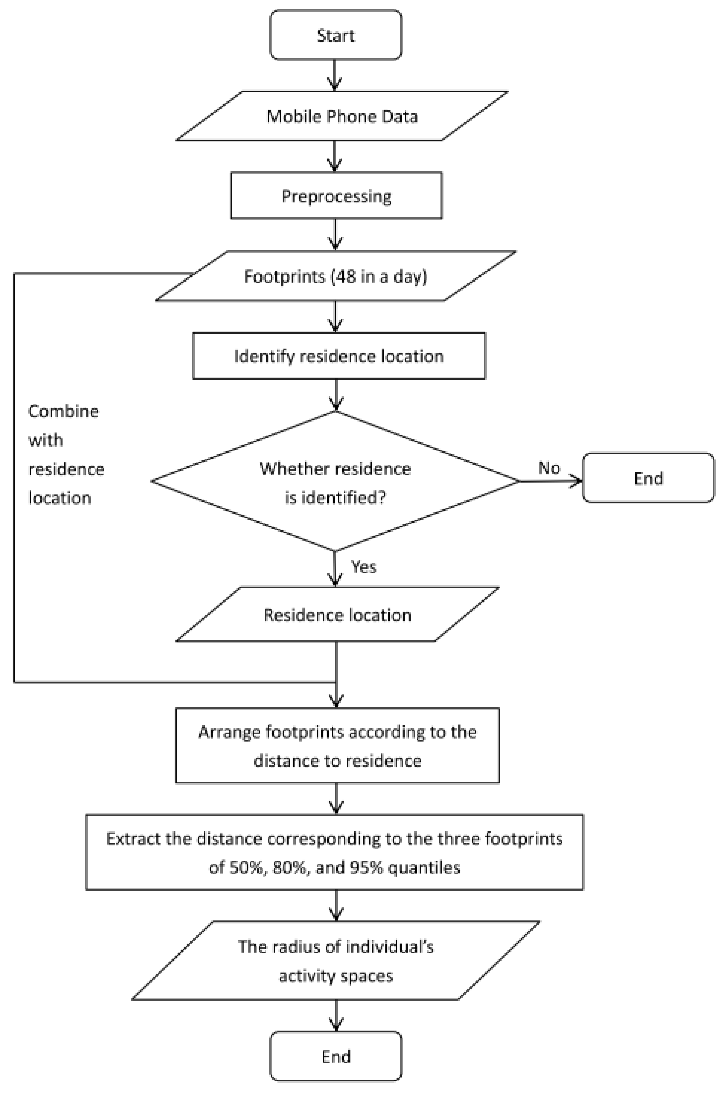
3.2. Activity Space Identifying Algorithm
3.3. Correspondence between Activity Space and Built Environment
4. Empirical Study
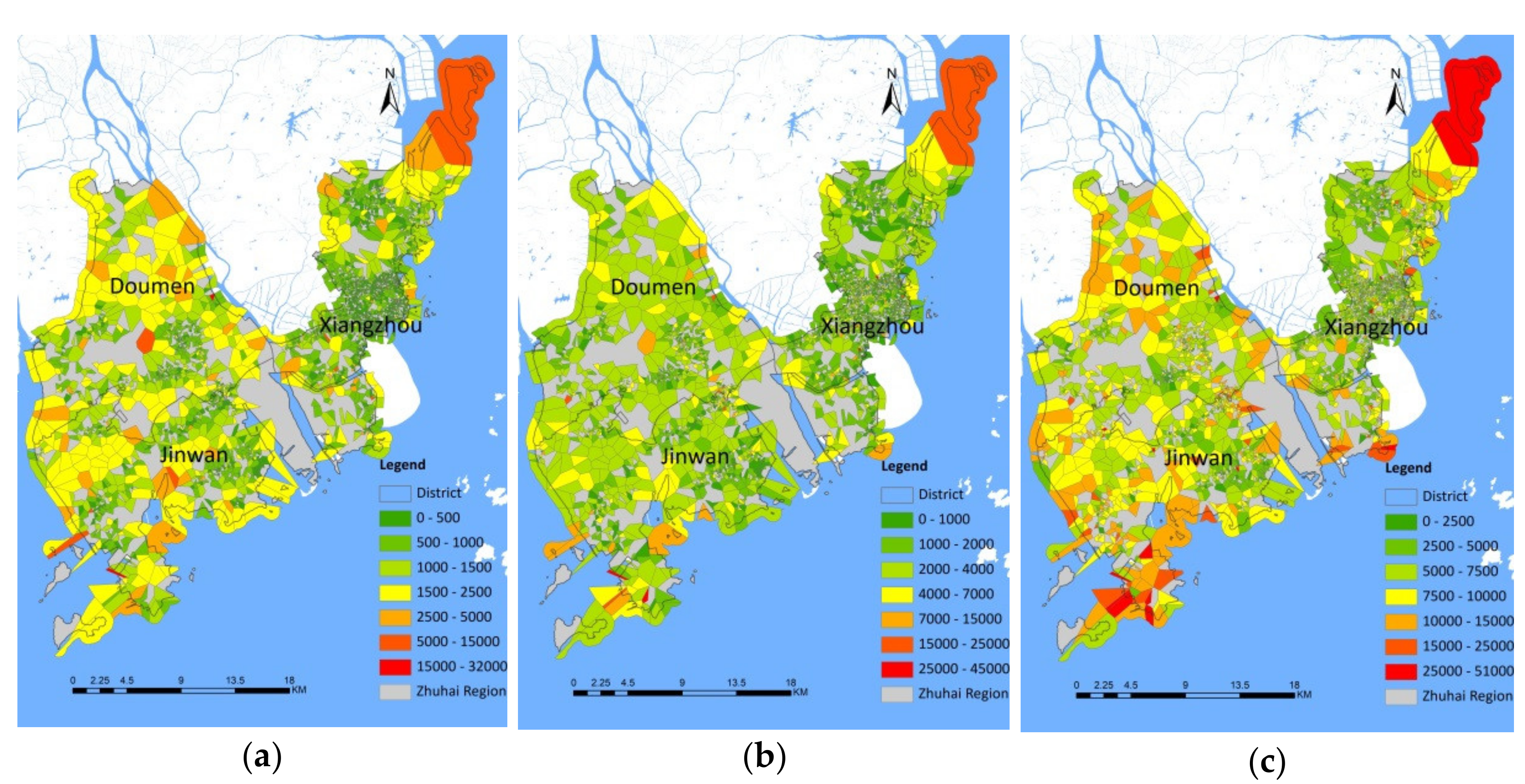
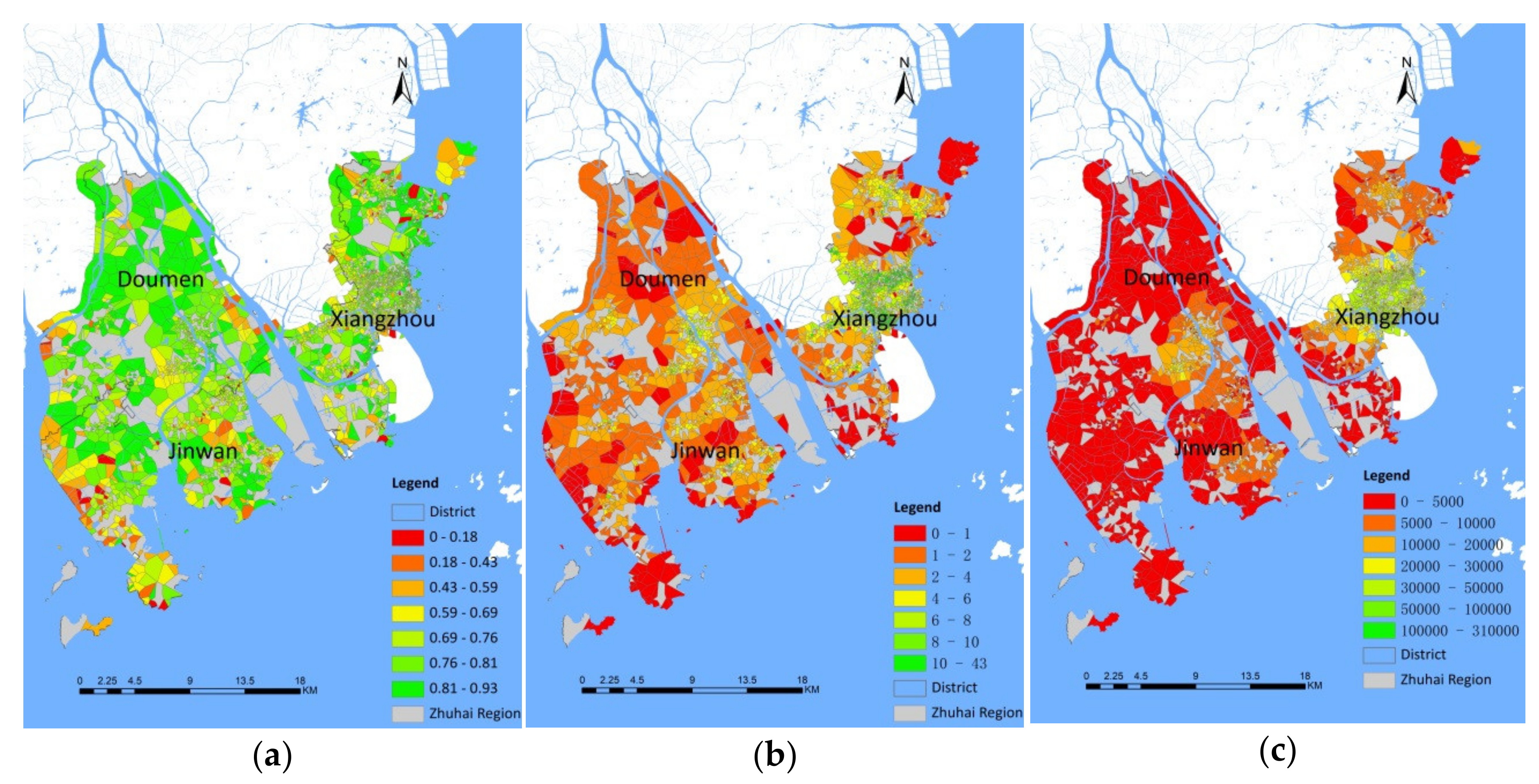
4.1. Activity Space Identification Result
4.2. Built Environment Factors and the Regression Model
4.3. Discussion
5. Conclusions
- We propose a multiple geographic scale activity space measuring method using the temporal duration of activities on the top of Time Geography theory and apply the massive mobile phone data on discovering the activity space at multiple geographic scales according to activity types. Using this method, the human activity space for multiple activities can be accurately captured and depicted. We also demonstrate the proposed method using Zhuhai mobile phone data.
- We analyze the relationship between activity space size and the built environment in detail at multiple geographic scales in Zhuhai. We find that different types of land-use affect the size of activity space differently. We also discover the positive relationship between POI diversity and the size of activity space at each geographic scale, which was much different from existing studies. This may be owed to the varying size of activity spaces defined by the average radius of the activity spaces of residents living in the spatial unit.
- In general, this research provides a method for measuring human activity space and can reveal the spatio-temporal characteristics of urban activities. For example, this method can identify areas with large activity space and dense population, which means that these areas need to build more functional facilities. Also, the findings from these results offer a better understanding of the relationships between the urban activity and the built environment at multiple geographic scales, revealing the main environmental factors that need to be built or improved. These can facilitate the urban planner to ameliorate the facility distributions for improving citizens’ life quality.
Author Contributions
Funding
Acknowledgments
Conflicts of Interest
References
- Golledge, R.G.; Stimson, R.J. Spatial Behavior: A Geographic Perspective; The Guilford Press: New York, NY, USA, 1997; pp. 277–282. [Google Scholar]
- Sherman, J.E.; Spencer, J.; Preisser, J.S.; Gesler, W.M.; Arcury, T.A. A suite of methods for representing activity space in a healthcare accessibility study. Int. J. Health Geogr. 2005, 4, 24. [Google Scholar] [CrossRef] [PubMed] [Green Version]
- Vallée, J.; Cadot, E.; Grillo, F.; Parizot, I.; Chauvin, P. The combined effects of activity space and neighbourhood of residence on participation in preventive health-care activities: The case of cervical screening in the paris metropolitan area (france). Health Place 2010, 16, 838–852. [Google Scholar] [CrossRef] [PubMed] [Green Version]
- Palmer, J.R.B. Activity-Space Segregation: Understanding Social Divisions in Space and Time. Ph.D. Thesis, Princeton University, Princeton, NJ, USA, 2013. [Google Scholar]
- Mason, M.J. Attributing activity space as risky and safe: The social dimension to the meaning of place for urban adolescents. Health Place 2010, 16, 926–933. [Google Scholar] [CrossRef] [PubMed] [Green Version]
- Kestens, Y.; Lebel, A.; Chaix, B.; Clary, C.; Daniel, M.; Pampalon, R.; Theriault, M.; Subramanian, S.V. Association between activity space exposure to food establishments and individual risk of overweight. PLoS ONE 2012, 7, e41418. [Google Scholar] [CrossRef]
- Hägerstrand, T. What about people in regional science? Pap. Reg. Sci. Assoc. 1970, 24, 6–21. [Google Scholar] [CrossRef]
- Congrès International d’Architecture Modern. Charter of Athens. In Proceedings of the 4th meeting of CIAM, Athens, The Hellenic Republic, 29 July–31 August 1933. [Google Scholar]
- Handy, S.L.; Boarnet, M.G.; Ewing, R.; Killingsworth, R.E. How the built environment affects physical activity: Views from urban planning. Am. J. Prev. Med. 2002, 23, 64–73. [Google Scholar] [CrossRef]
- Yang, L.; Hu, L.; Wang, Z. The built environment and trip chaining behaviour revisited: The joint effects of the modifiable areal unit problem and tour purpose. Urban Stud. 2019, 56, 795–817. [Google Scholar] [CrossRef]
- Golledge, R.G. Learning about urban environments. In Timing Space and Spacing Time; Parkes, D.N., Thrift, N., Eds.; Edward Arnold: London, UK, 1978. [Google Scholar]
- Bagrow, J.P.; Koren, T. Investigating bimodal clustering in human mobility. In Proceedings of the International Conference on Computational Science and Engineering, Vancouver, BC, Canada, 29–31 August 2009; Volume 4, pp. 944–947. [Google Scholar]
- Kutter, E. A model for individual travel behaviour. Urban Stud. 1973, 10, 235–258. [Google Scholar] [CrossRef]
- Roof, K.; Oleru, N. Public health: Seattle and King County’s push for the built environment. J. Environ. Health 2008, 71, 24–27. [Google Scholar]
- Boarnet, M.; Crane, R. The influence of land use on travel behavior: Specification and estimation strategies. Transp. Res. Part A Policy Pract. 2001, 35, 823–845. [Google Scholar] [CrossRef]
- Cervero, R.; Kockelman, K. Travel demand and the 3Ds: Density, diversity, and design. Transp. Res. Part D Transp. Environ. 1997, 2, 199–219. [Google Scholar] [CrossRef]
- Cao, X.J.; Mokhtarian, P.L.; Handy, S.L. The relationship between the built environment and nonwork travel: A case study of Northern California. Transp. Res. Part A Policy Pract. 2009, 43, 548–559. [Google Scholar] [CrossRef]
- Pushkar, A.O.; Hollingworth, B.J.; Miller, E.J. A multivariate regression model for estimating greenhouse gas emissions from alternative neighborhood designs. In Proceedings of the 79th Annual Meeting of the Transportation Research Board, Washington, DC, USA, 9–13 January 2000. [Google Scholar]
- Haybatollahi, M.; Czepkiewicz, M.; Laatikainen, T.; Kyttä, M. Neighbourhood preferences, active travel behaviour, and built environment: An exploratory study. Transp. Res. Part F Traffic Psychol. Behav. 2015, 29, 57–69. [Google Scholar] [CrossRef]
- Alfonzo, M.; Boarnet, M.G.; Day, K.; Mcmillan, T.; Anderson, C.L. The relationship of neighbourhood built environment features and adult parents’ walking. J. Urban Des. 2008, 13, 29–51. [Google Scholar] [CrossRef]
- Cervero, R. Built environments and mode choice: Toward a normative framework. Transp. Res. Part D Transp. Environ. 2002, 7, 265–284. [Google Scholar] [CrossRef]
- Levinson, D.M.; Kumar, A. Density and the journey to work. Growth Chang. 1997, 28, 147–172. [Google Scholar] [CrossRef]
- Schwanen, T. The impact of metropolitan structure on commute behavior in the netherlands: A multilevel approach. Growth Chang. 2010, 35, 304–333. [Google Scholar] [CrossRef]
- Moilanen, M. Matching and settlement patterns: The case of norway. Pap. Reg. Sci. 2010, 89, 607–623. [Google Scholar] [CrossRef]
- Schwanen, T.; Ettema, D.; Timmermans, H. If you pick up the children, I’ll do the groceries: Spatial differences in between-partner interactions in out-of-home household activities. Environ. Plan. A 2007, 39, 2754–2773. [Google Scholar] [CrossRef]
- Xu, Y.; Shaw, S.L.; Zhao, Z.; Yin, L.; Fang, Z.; Li, Q. Understanding aggregate human mobility patterns using passive mobile phone location data: A home-based approach. Transportation 2015, 42, 625–646. [Google Scholar] [CrossRef]
- Kang, C.; Liu, Y.; Ma, X.; Wu, L. Towards estimating urban population distributions from mobile call data. J. Urban Technol. 2012, 19, 3–21. [Google Scholar] [CrossRef]
- Xu, Y.; Shaw, S.L.; Zhao, Z.; Yin, L.; Lu, F.; Chen, J.; Fang, Z.; Li, Q. Another tale of two cities: Understanding human activity space using actively tracked cellphone location data. Ann. Am. Assoc. Geogr. 2016, 106, 489–502. [Google Scholar]
- Yuan, Y.; Raubal, M. Analyzing the distribution of human activity space from mobile phone usage: An individual and urban-oriented study. Int. J. Geogr. Inf. Sci. 2016, 30, 1594–1621. [Google Scholar] [CrossRef]
- Calabrese, F.; Diao, M.; Di Lorenzo, G.; Ferreira, J., Jr.; Ratti, C. Understanding individual mobility patterns from urban sensing data: A mobile phone trace example. Transp. Res. Part C Emerg. Technol. 2013, 26, 301–313. [Google Scholar] [CrossRef]
- Saelens, B.E.; Handy, S.L. Built environment correlates of walking: A review. Med. Sci. Sports Exerc. 2008, 40, S550. [Google Scholar] [CrossRef] [Green Version]
- Yue, Y.; Zhuang, Y.; Yeh, A.G.O.; Xie, J.Y.; Ma, C.L.; Li, Q.Q. Measurements of poi-based mixed use and their relationships with neighbourhood vibrancy. Int. J. Geogr. Inf. Sci. 2017, 31, 658–675. [Google Scholar] [CrossRef] [Green Version]
- Srinivasan, S.; Bhat, C.R. Modeling household interactions in daily in-home and out-of-home maintenance activity participation. Transportation 2005, 32, 523–544. [Google Scholar] [CrossRef] [Green Version]
- Schönfelder, S.; Axhausen, K.W. Activity spaces: Measures of social exclusion? Transp. Policy 2003, 10, 273–286. [Google Scholar] [CrossRef] [Green Version]
- Ham, S.A.; Kruger, J.; Tudor-Locke, C. Participation by US adults in sports, exercise, and recreational physical activities. J. Phys. Act. Health 2009, 6, 6–14. [Google Scholar] [CrossRef]
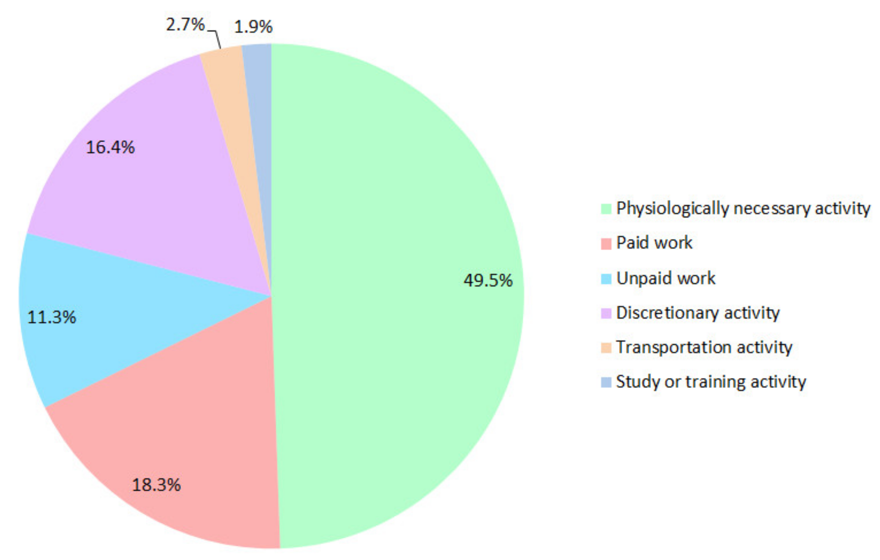
- Bureau of Statistics of China. The 2018 National Time Utilization Survey Bulletin. China Statistics 2019, 2, 10–14. [Google Scholar]
- Ren, M.; Lin, Y.; Jin, M.; Duan, Z.; Gong, Y.; Liu, Y. Examining the effect of land-use function complementarity on intra-urban spatial interactions using metro smart card records. Transportation 2019. [Google Scholar] [CrossRef]
- Shiftan, Y.; Barlach, Y. Effect of employment site characteristics on commute mode choice. Transp. Res. Rec. 2002, 1781, 19–25. [Google Scholar] [CrossRef]
- Zhang, M. The role of land use in travel mode choice: Evidence from Boston and Hong Kong. J. Am. Plan. Assoc. 2004, 70, 344–360. [Google Scholar] [CrossRef]
- Greenwald, M.J.; Boarnet, M.G. Built environment as determinant of walking behavior: Analyzing nonwork pedestrian travel in Portland, Oregon. Transp. Res. Record. 2001, 1780, 33–41. [Google Scholar] [CrossRef] [Green Version]
- Bichler, G.; Christie-Merrall, J.; Sechrest, D. Examining juvenile delinquency within activity space: Building a context for offender travel patterns. J. Res. Crime Delinq. 2011, 48, 472–506. [Google Scholar] [CrossRef]
- Boussauw, K.; Neutens, T.; Witlox, F. Relationship between spatial proximity and travel-to-work distance: The effect of the compact city. Reg. Stud. 2012, 46, 687–706. [Google Scholar] [CrossRef]


| Primary Categories | Subcategories | Numbers |
|---|---|---|
| Consumption | Catering Shopping Recreation Accommodation Comprehensive | 19,242 37,745 2652 2213 18,812 |
| Corporation | Corporation | 17,000 |
| Public service | Government and social groups Park and square Public facility Hospital and pharmacy | 3494 573 671 3394 |
| Traffic | Transportation facility | 4416 |
| Education | Educational and scientific service | 3555 |
| Residence | Residence | 3292 |
| Variables | Model 1 | Model 2 | Model 3 |
|---|---|---|---|
| (Maintenance) | (Commuting) | (Recreational) | |
| Catering | √ | - | - |
| Shopping | √ | - | - |
| Recreation | - | - | √ |
| Comprehensive | - | - | √ |
| Public facility | - | - | √ |
| Educational and scientific service | - | √ | - |
| Residence | √ | √ | - |
| POI diversity | √ | √ | √ |
| Distance to city center | √ | - | √ |
| Road network density | √ | √ | - |
| Working population density | - | √ | - |
| Variables | Model 1 | Model 2 | Model 3 | |||
|---|---|---|---|---|---|---|
| Mean | Std. | Mean | Std. | Mean | Std. | |
| Catering | 125.944 | 227.684 | 73.901 | 125.575 | 51.676 | 94.139 |
| Shopping | 247.603 | 737.304 | 137.854 | 297.888 | 96.012 | 187.692 |
| Recreation | 16.697 | 29.084 | 10.353 | 16.288 | 7.104 | 10.681 |
| Comprehensive | 15.037 | 38.174 | 8.799 | 17.798 | 5.965 | 12.159 |
| Public facility | 3.538 | 7.863 | 2.315 | 4.260 | 1.641 | 3.282 |
| Educational and- Scientific service | 22.442 | 42.756 | 14.121 | 24.733 | 10.065 | 17.326 |
| Residence | 18.897 | 32.632 | 11.403 | 21.070 | 8.185 | 18.233 |
| POI Diversity | 0.067 | 0.040 | 0.074 | 0.024 | 0.075 | 0.017 |
| Distance to city- Center | 16.889 | 14.733 | 16.889 | 14.733 | 16.889 | 14.733 |
| Road network density | 6.839 | 5.188 | 67.326 | 733.822 | 3.727 | 2.640 |
| Working population- Density | 125.944 | 227.684 | 73.901 | 125.575 | 51.676 | 94.139 |
| Model | Standardization Coefficient | Sig. | Adjust R2 |
|---|---|---|---|
| Model 1 (Maintenance) | |||
| Catering | −0.047 | 0.010 | 0.514 |
| Shopping | −0.059 | 0.000 | |
| Residence | −0.111 | 0.000 | |
| POI Diversity | 0.354 | 0.000 | |
| Distance to city center | 0.255 | 0.000 | |
| Road network density | −0.434 | 0.000 | |
| Model 2 (Commuting) | |||
| Educational and- scientific service | −0.088 | 0.000 | 0.524 |
| Working population- density | 0.085 | 0.000 | |
| POI diversity | 0.443 | 0.000 | |
| Distance to city center | 0.095 | 0.000 | |
| Road network density | −0.517 | 0.000 | |
| Model 3 (Recreational) | |||
| Recreation | −0.394 | 0.000 | 0.458 |
| Comprehensive | −0.212 | 0.000 | |
| POI Diversity | 0.440 | 0.000 | |
| Distance to city center | 0.012 | 0.422 | |
| Public facility | 0.287 | 0.000 |
| Model 1 | Model 2 | Model 3 | |||
|---|---|---|---|---|---|
| Variables | VIF | Variables | VIF | Variables | VIF |
| Catering | 2.262 | Educational and- scientific service | 1.005 | Recreation | 10.104 |
| Shopping | 1.620 | Working population- density | 2.120 | Comprehensive | 3.244 |
| Residence | 1.217 | POI density | 1.027 | Diversity | 1.153 |
| POI density | 1.046 | Distance to city center | 1.912 | Distance to city center | 1.292 |
| Distance to- city center | 1.343 | Road density | 1.659 | Public facility | 6.100 |
| Road density | 1.722 | ||||
| Model | Coefficient | Sig. |
|---|---|---|
| Maintenance activity space | −0.618 | 0.000 |
| Commuting activity space | −1.413 | 0.000 |
| Recreational activity space | −1.363 | 0.000 |
© 2020 by the authors. Licensee MDPI, Basel, Switzerland. This article is an open access article distributed under the terms and conditions of the Creative Commons Attribution (CC BY) license (http://creativecommons.org/licenses/by/4.0/).
Share and Cite
Gong, L.; Jin, M.; Liu, Q.; Gong, Y.; Liu, Y. Identifying Urban Residents’ Activity Space at Multiple Geographic Scales Using Mobile Phone Data. ISPRS Int. J. Geo-Inf. 2020, 9, 241. https://0-doi-org.brum.beds.ac.uk/10.3390/ijgi9040241
Gong L, Jin M, Liu Q, Gong Y, Liu Y. Identifying Urban Residents’ Activity Space at Multiple Geographic Scales Using Mobile Phone Data. ISPRS International Journal of Geo-Information. 2020; 9(4):241. https://0-doi-org.brum.beds.ac.uk/10.3390/ijgi9040241
Chicago/Turabian StyleGong, Lunsheng, Meihan Jin, Qiang Liu, Yongxi Gong, and Yu Liu. 2020. "Identifying Urban Residents’ Activity Space at Multiple Geographic Scales Using Mobile Phone Data" ISPRS International Journal of Geo-Information 9, no. 4: 241. https://0-doi-org.brum.beds.ac.uk/10.3390/ijgi9040241