Ambient Population and Larceny-Theft: A Spatial Analysis Using Mobile Phone Data

 , ,
, ,
Abstract
:1. Introduction
2. Background
2.1. Ambient Population in Crime Analysis
2.2. Mobile Phone Data for Crime Analysis
2.3. Routine Activity Theory
2.4. Crime Pattern Theory
3. Study Area, Data, and Methods
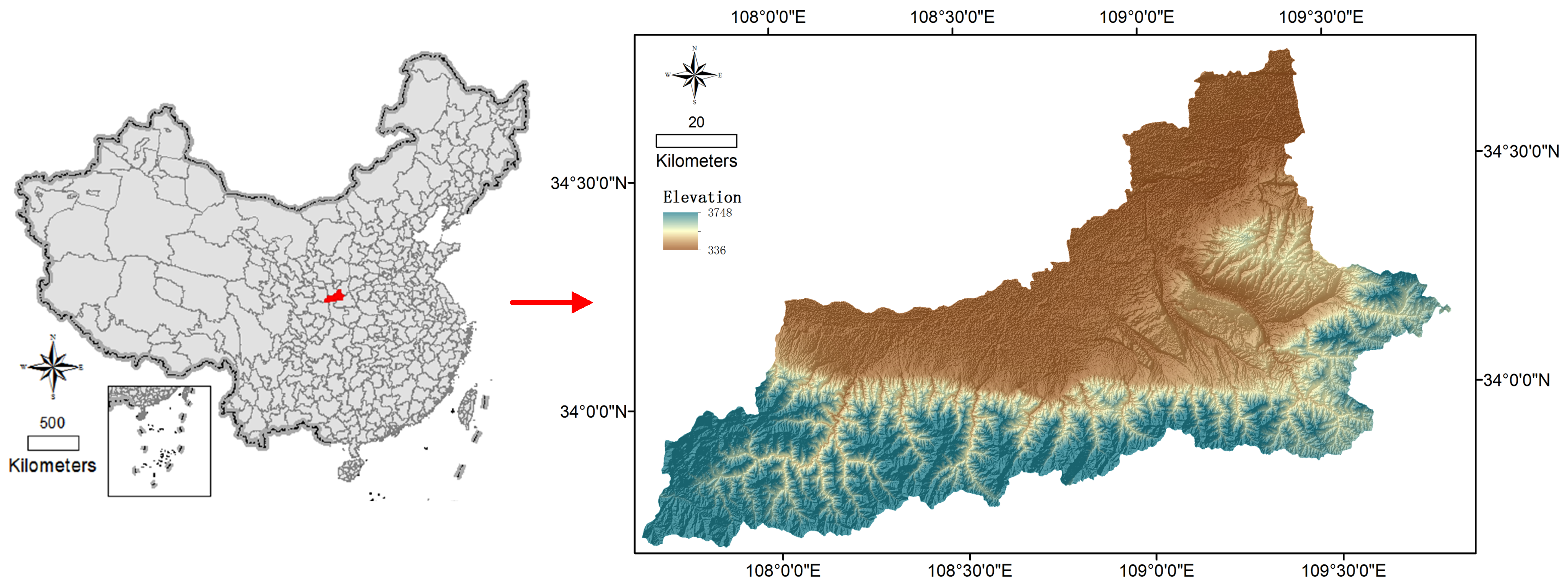
3.1. Study Area
3.2. Data
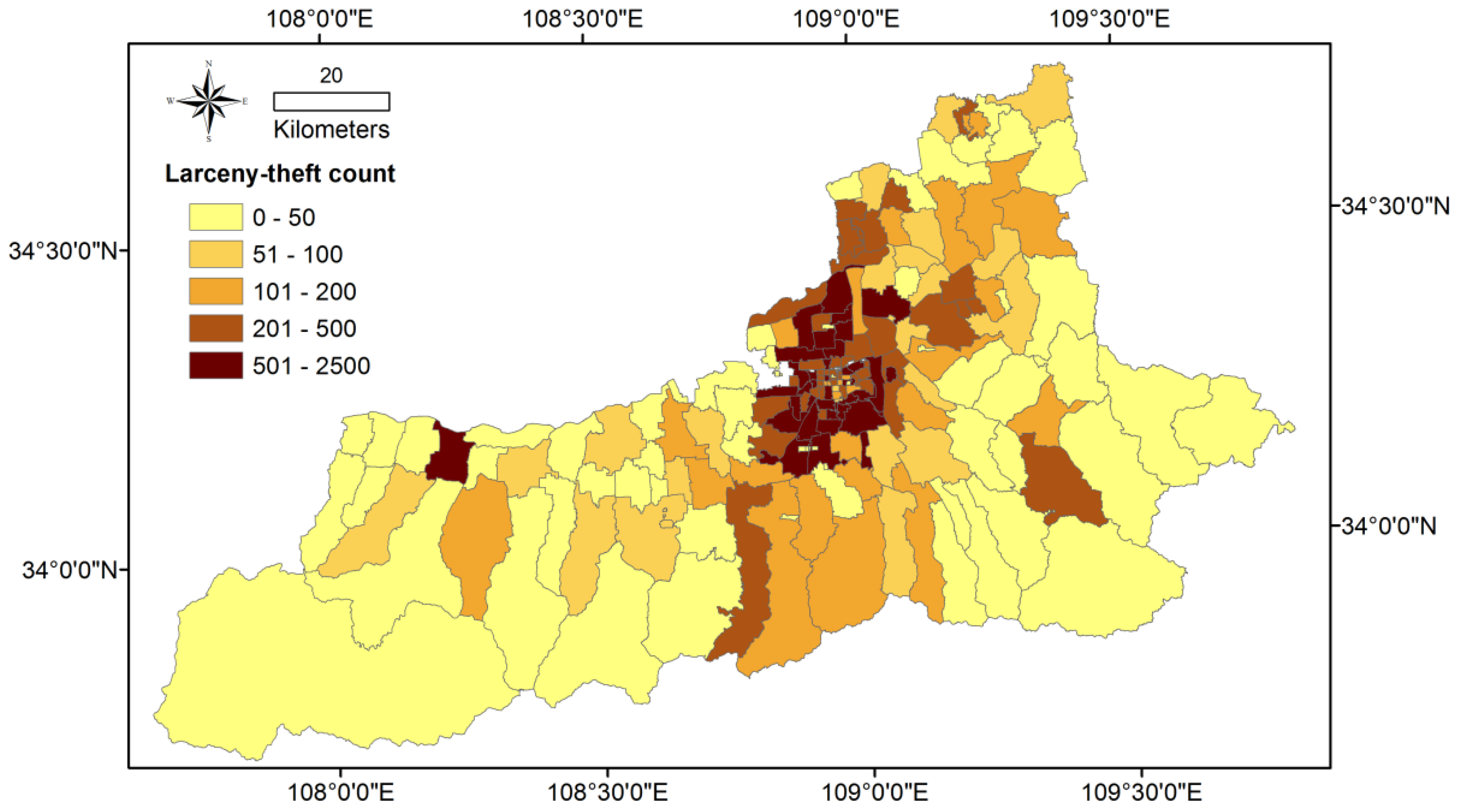
3.2.1. Crime Data
3.2.2. Spatially Referenced Mobile Phone Big Data
3.2.3. Point of Interest (POI) Data
3.2.4. Luojia 1-01 Nighttime Light Imaging
3.3. Methods
3.3.1. Exploratory Spatial Data Analysis
3.3.2. Negative Binomial Regression
4. Analysis and Results
4.1. Exploratory Spatial Data Analysis
4.2. Regression Analysis
5. Discussion
6. Conclusions
Supplementary Materials
Author Contributions
Funding
Acknowledgments
Conflicts of Interest
References
- Andresen, M.A. The Ambient Population and Crime Analysis. Prof. Geogr. 2011, 63, 193–212. [Google Scholar] [CrossRef]
- Malleson, N.; Andresen, M.A. The impact of using social media data in crime rate calculations: Shifting hot spots and changing spatial patterns. Cartogr. Geogr. Inf. Sc. 2015, 42, 112–121. [Google Scholar] [CrossRef]
- Malleson, N.; Andresen, M.A. Exploring the impact of ambient population measures on London crime hotspots. J. Crim. Justice 2016, 46, 52–63. [Google Scholar] [CrossRef] [Green Version]
- Hanaoka, K. New insights on relationships between street crimes and ambient population: Use of hourly population data estimated from mobile phone users’ locations. Environ. Plan. B Urban Anal. City Sci. 2016, 45, 295–311. [Google Scholar] [CrossRef]
- Song, G.; Liu, L.; Bernasco, W.; Xiao, L.; Zhou, S.; Liao, W. Testing Indicators of Risk Populations for Theft from the Person across Space and Time: The Significance of Mobility and Outdoor Activity. Ann. Am. Assoc. Geogr. 2018, 108, 1370–1388. [Google Scholar] [CrossRef]
- Deville, P.; Linard, C.; Martin, S.; Gilbert, M.; Stevens, F.R.; Gaughan, A.E.; Blondel, V.D.; Tatem, A.J. Dynamic population mapping using mobile phone data. Proc. Natl. Acad. Sci. 2014, 111, 15888–15893. [Google Scholar] [CrossRef] [Green Version]
- Hipp, J.; Bates, C.; Lichman, M.; Smyth, P. Using Social Media to Measure Temporal Ambient Population: Does it Help Explain Local Crime Rates? Justice Q. 2018, 36, 1–31. [Google Scholar] [CrossRef] [Green Version]
- Kinney, J.B.; Brantingham, P.L.; Wuschke, K.; Kirk, M.G.; Brantingham, P.J. Crime Attractors, Generators and Detractors: Land Use and Urban Crime Opportunities. Built Environ. 2008, 34, 62–74. [Google Scholar] [CrossRef]
- Brantingham, P.L.; Brantingham, P.J. Criminality of place: Crime generators and crime attractors. Eur. J. Crim. Pol. Res. 1995, 3, 1–26. [Google Scholar] [CrossRef]
- Felson, L.E.C. Social Change and Crime Rate Trends: A Routine Activity Approach. Am. Sociol. Rev. 1979, 44, 588. [Google Scholar] [CrossRef]
- Morency, C.; Páez, A.; Roorda, M.; Mercado, R.; Farber, S. Distance traveled in three Canadian cities: Spatial analysis from the perspective of vulnerable population segments. J. Transp. Geogr. 2011, 19, 39–50. [Google Scholar] [CrossRef]
- Clarke, R.V. OPPORTUNITY-BASED CRIME RATESThe Diffculties of Further Refinement. Br. J. Criminol. 1984, 24, 74–83. [Google Scholar] [CrossRef]
- Andresen, M.A. Location Quotients, Ambient Populations, and the Spatial Analysis of Crime in Vancouver, Canada. Environ. Plan. A: Econ. Space 2007, 39, 2423–2444. [Google Scholar] [CrossRef]
- Liu, L.; Jiang, C.; Zhou, S.; Liu, K.; Du, F. Impact of public bus system on spatial burglary patterns in a Chinese urban context. Appl. Geogr. 2017, 89, 142–149. [Google Scholar] [CrossRef]
- Lan, M.; Liu, L.; Hernandez, A.; Liu, W.; Zhou, H.; Wang, Z. The Spillover Effect of Geotagged Tweets as a Measure of Ambient Population for Theft Crime. Sustainability 2019, 11, 6748. [Google Scholar] [CrossRef] [Green Version]
- Crols, T.; Malleson, N. Quantifying the ambient population using hourly population footfall data and an agent-based model of daily mobility. GeoInformatica 2019, 23, 201–220. [Google Scholar] [CrossRef] [Green Version]
- Li, T.; Sun, D.; Jing, P.; Yang, K. Smart Card Data Mining of Public Transport Destination: A Literature Review. Information 2018, 9, 18. [Google Scholar] [CrossRef] [Green Version]
- Dobson, J.E.; Bright, E.A.; Coleman, P.R.; Durfee, R.C.; Worley, B.A. LandScan: A global population database for estimating populations at risk. Photogramm. Eng. Rem. S. 2000, 66, 849–857. [Google Scholar]
- Bowers, K.J.; Johnson, S.D.; Pease, K. Prospective Hot-Spotting: The Future of Crime Mapping? Br. J. Criminol. 2004, 44, 641–658. [Google Scholar] [CrossRef]
- Shiode, S. Street-level Spatial Scan Statistic and STAC for Analysing Street Crime Concentrations. Trans. GIS 2011, 15, 365–383. [Google Scholar] [CrossRef]
- Vespignani, A. Predicting the Behavior of Techno-Social Systems. Science 2009, 325, 425–428. [Google Scholar] [CrossRef]
- Lazer, D.; Pentland, A. (Sandy); Adamic, L.; Aral, S.; Barabasi, A.-L.; Brewer, D.; Christakis, N.; Contractor, N.; Fowler, J.H.; Gutmann, M.; et al. SOCIAL SCIENCE: Computational Social Science. Science 2009, 323, 721–723. [Google Scholar] [CrossRef] [PubMed] [Green Version]
- Liu, Y.; Liu, X.; Gao, S.; Gong, L.; Kang, C.; Zhi, Y.; Chi, G.; Shi, L. Social Sensing: A New Approach to Understanding Our Socioeconomic Environments. Ann. Assoc. Am. Geogr. 2015, 105, 512–530. [Google Scholar] [CrossRef]
- Panigutti, C.; Tizzoni, M.; Bajardi, P.; Smoreda, Z.; Colizza, V. Assessing the use of mobile phone data to describe recurrent mobility patterns in spatial epidemic models. R. Soc. Open Sci. 2017, 4, 160950. [Google Scholar] [CrossRef] [PubMed] [Green Version]
- González, M.C.; Pinheiro, F.L.; Barabasi, A.-L. Understanding individual human mobility patterns. Nature 2008, 453, 779–782. [Google Scholar] [CrossRef]
- Song, G.; Bernasco, W.; Liu, L.; Xiao, L.; Zhou, S.; Liao, W. Crime Feeds on Legal Activities: Daily Mobility Flows Help to Explain Thieves’ Target Location Choices. J. Quant. Criminol. 2019, 35, 831–854. [Google Scholar] [CrossRef] [Green Version]
- Griffiths, G.; Johnson, S.D.; Chetty, K. UK-based terrorists’ antecedent behavior: A spatial and temporal analysis. Appl. Geogr. 2017, 86, 274–282. [Google Scholar] [CrossRef]
- Bogomolov, A.; Lepri, B.; Staiano, J.; Oliver, N.; Pianesi, F.; Pentland, A. Once Upon a Crime: Towards Crime Prediction from Demographics and Mobile Data. In Proceedings of the 16th International Conference on Multimodal Interaction; Istanbul, Turkey, 12–16 November 2014, Association for Computing Machinery: Istanbul, Turkey; pp. 427–434.
- Reades, J.; Calabrese, F.; Ratti, C. Eigenplaces: Analysing cities using the space – time structure of the mobile phone network. Environ. Plan. B Plan. Des. 2009, 36, 824–836. [Google Scholar] [CrossRef] [Green Version]
- Dhondt, S.; Beckx, C.; Degraeuwe, B.; Lefebvre, W.; Kochan, B.; Bellemans, T.; Panis, L.I.; Macharis, C.; Putman, K. Integration of population mobility in the evaluation of air quality measures on local and regional scales. Atmospheric Environ. 2012, 59, 67–74. [Google Scholar] [CrossRef]
- He, L.; Páez, A.; Liu, D. Built environment and violent crime: An environmental audit approach using Google Street View. Comput. Environ. Urban Syst. 2017, 66, 83–95. [Google Scholar] [CrossRef]
- Eck, J.E.; Weisburd, D. Crime Places in Crime Theory. In Crime and Place, crime Prevention Studies; Eck, J.E., Weisburd, D., Eds.; Criminal Justice Press: Monsey, NY, USA, 1995. [Google Scholar]
- Sherman, L.W.; Gartin, P.R.; Buerger, M.E. HOT SPOTS OF PREDATORY CRIME: ROUTINE ACTIVITIES AND THE CRIMINOLOGY OF PLACE*. Criminology 1989, 27, 27–56. [Google Scholar] [CrossRef]
- Cozens, P.; Love, T.; Nasar, J.L. A Review and Current Status of Crime Prevention through Environmental Design (CPTED). J. Plan. Lit. 2015, 30, 393–412. [Google Scholar] [CrossRef]
- Wilcox, P.; Quisenberry, N.; Cabrera, D.T.; Jones, A. Busy Places and Broken Windows? Toward Defining the Role of Physical Structure and Process in Community Crime Models. Sociol. Q. 2004, 45, 185–207. [Google Scholar] [CrossRef]
- Andresen, M.A. Crime measures and the spatial analysis of criminal activity. Brit. J. Criminol. 2006, 46, 258–285. [Google Scholar] [CrossRef]
- He, L.; Páez, A.; Liu, D.; Jiang, S. Temporal stability of model parameters in crime rate analysis: An empirical examination. Appl. Geogr. 2015, 58, 141–152. [Google Scholar] [CrossRef]
- He, L.; Páez, A.; Liu, D. Persistence of Crime Hot Spots: An Ordered Probit Analysis. Geogr. Anal. 2016, 49, 3–22. [Google Scholar] [CrossRef] [Green Version]
- Bernasco, W.; Block, R.; Rengert, G.; Groff, E.; Eck, J. Robberies in Chicago: A Block-Level Analysis of the Influence of Crime Generators, Crime Attractors, and Offender Anchor Points. J. Res. Crime Delinquency 2010, 48, 33–57. [Google Scholar] [CrossRef]
- Mburu, L.W.; Helbich, M. Environmental Risk Factors influencing Bicycle Theft: A Spatial Analysis in London, UK. PLoS ONE 2016, 11, e0163354. [Google Scholar] [CrossRef] [Green Version]
- Sypion-Dutkowska, N.; Leitner, M. Land Use Influencing the Spatial Distribution of Urban Crime: A Case Study of Szczecin, Poland. ISPRS Int. J. Geo-Information 2017, 6, 74. [Google Scholar] [CrossRef] [Green Version]
- Roncek, D.W.; Maier, P.A. BARS, BLOCKS, AND CRIMES REVISITED: LINKING THE THEORY OF ROUTINE ACTIVITIES TO THE EMPIRICISM OF "HOT SPOTS"*. Criminology 1991, 29, 725–753. [Google Scholar] [CrossRef]
- Stucky, T.D.; Ottensmann, J.R. LAND USE AND VIOLENT CRIME*. Criminology 2009, 47, 1223–1264. [Google Scholar] [CrossRef] [Green Version]
- Browning, C.R.; Byron, R.A.; Calder, C.; Krivo, L.J.; Kwan, M.-P.; Lee, J.-Y.; Peterson, R.D. Commercial Density, Residential Concentration, and Crime: Land Use Patterns and Violence in Neighborhood Context. J. Res. Crime Delinquency 2010, 47, 329–357. [Google Scholar] [CrossRef]
- Song, G.; Liu, L.; Bernasco, W.; Zhou, S.; Xiao, L.; Long, D. Theft from the person in urban China: Assessing the diurnal effects of opportunity and social ecology. Habitat Int. 2018, 78, 13–20. [Google Scholar] [CrossRef]
- Feng, J.; Liu, L.; Long, D.; Liao, W. An Examination of Spatial Differences between Migrant and Native Offenders in Committing Violent Crimes in a Large Chinese City. ISPRS Int. J. Geo-Information 2019, 8, 119. [Google Scholar] [CrossRef] [Green Version]
- Steffensmeier, D.; Harris, C.T.; Painter-Davis, N. Gender and Arrests for Larceny, Fraud, Forgery, and Embezzlement: Conventional or Occupational Property Crime Offenders? J. Crim. Justice 2015, 43, 205–217. [Google Scholar] [CrossRef]
- Cabrera-Barona, P.; Pontón, G.J.; Melo, P. Types of Crime, Poverty, Population Density and Presence of Police in the Metropolitan District of Quito. ISPRS Int. J. Geo-Inf. 2019, 8, 558. [Google Scholar] [CrossRef] [Green Version]
- Chen, J.; Liu, L.; Zhou, S.; Xiao, L.; Jiang, C. Spatial Variation Relationship between Floating Population and Residential Burglary: A Case Study from ZG, China. ISPRS Int. J. Geo-Inf. 2017, 6, 246. [Google Scholar] [CrossRef] [Green Version]
- Chen, J.; Liu, L.; Xiao, L.; Xu, C.; Long, D. Integrative Analysis of Spatial Heterogeneity and Overdispersion of Crime with a Geographically Weighted Negative Binomial Model. ISPRS Int. J. Geo-Inf. 2020, 9, 60. [Google Scholar] [CrossRef] [Green Version]
- Papa, G.L.; Palermo, V.; Dazzi, C. Is land-use change a cause of loss of pedodiversity? The case of the Mazzarrone study area, Sicily. Geomorphology 2011, 135, 332–342. [Google Scholar] [CrossRef]
- Shi, K.; Yu, B.; Huang, Y.; Hu, Y.; Yin, B.; Chen, Z.; Chen, L.; Wu, J. Evaluating the Ability of NPP-VIIRS Nighttime Light Data to Estimate the Gross Domestic Product and the Electric Power Consumption of China at Multiple Scales: A Comparison with DMSP-OLS Data. Remote. Sens. 2014, 6, 1705–1724. [Google Scholar] [CrossRef] [Green Version]
- Bruederle, A.; Hodler, R. Nighttime lights as a proxy for human development at the local level. PLoS ONE 2018, 13, e0202231. [Google Scholar] [CrossRef] [PubMed] [Green Version]
- Yin, Z.; Li, X.; Tong, F.; Li, Z.; Jendryke, M. Mapping urban expansion using night-time light images from Luojia1-01 and International Space Station. Int. J. Remote. Sens. 2019, 41, 2603–2623. [Google Scholar] [CrossRef]
- Zhou, H.; Liu, L.; Lan, M.; Yang, B.; Wang, Z. Assessing the Impact of Nightlight Gradients on Street Robbery and Burglary in Cincinnati of Ohio State, USA. Remote. Sens. 2019, 11, 1958. [Google Scholar] [CrossRef] [Green Version]
- Griffith, D.A. Spatial Autocorrelation and Spatial Filtering: Gaining Understanding through Theory and Scientific Visualization; Springer: Berlin, Germany, 2003. [Google Scholar]
- Moran, P.A.P. Notes on Continuous Stochastic Phenomena. Biometrika 1950, 37, 17. [Google Scholar] [CrossRef] [PubMed]
- Cliff, A.D.; Griffith, D.A.; Amrhein, C.G. Multivariate Statistical Analysis for Geographers. J. Am. Stat. Assoc. 1999, 94, 654. [Google Scholar] [CrossRef]
- Osgood, D.W. Poisson-Based Regression Analysis of Aggregate Crime Rates. J. Quant. Criminol. 2000, 16, 21–43. [Google Scholar] [CrossRef]
- Anselin, L.; Syabri, I.; Kho, Y. GeoDa: An Introduction to Spatial Data Analysis. Geogr. Anal. 2006, 38, 5–22. [Google Scholar] [CrossRef]
- Ranjan, C.; Najari, V. ProcessMiner/nlcor: Compute Nonlinear Correlations. 2019. Available online: https://github.com/ProcessMiner/nlcor (accessed on 16 April 2020).
- Glaeser, E.L.; Sacerdote, B. Why is There More Crime in Cities? J. Politi- Econ. 1999, 107, S225–S258. [Google Scholar] [CrossRef] [Green Version]
- Chang, Y.S.; Kim, H.E.; Jeon, S. Do Larger Cities Experience Lower Crime Rates? A Scaling Analysis of 758 Cities in the US. Sustainability 2019, 11, 3111. [Google Scholar] [CrossRef] [Green Version]
- Ladbrook, D.A. Why are crime rates higher in urban than in rural areas? — Evidence from Japan. Aust. N. Zealand J. Criminol. 1988, 21, 81–103. [Google Scholar] [CrossRef]
- Sampson, R.J.; Groves, W.B. Community Structure and Crime: Testing Social-Disorganization Theory. Am. J. Sociol. 1989, 94, 774–802. [Google Scholar] [CrossRef] [Green Version]
- Chun, Y. Analyzing Space-Time Crime Incidents Using Eigenvector Spatial Filtering: An Application to Vehicle Burglary. Geogr. Anal. 2014, 46, 165–184. [Google Scholar] [CrossRef]
- Sampson, R.J.; Raudenbush, S.W. Systematic Social Observation of Public Spaces: A New Look at Disorder in Urban Neighborhoods. Am. J. Sociol. 1999, 105, 603–651. [Google Scholar] [CrossRef] [Green Version]
- Bursik, R.J. SOCIAL DISORGANIZATION AND THEORIES OF CRIME AND DELINQUENCY: PROBLEMS AND PROSPECTS*. Criminology 1988, 26, 519–552. [Google Scholar] [CrossRef]
- Marcum, C.D.; Higgins, G.E.; Ricketts, M.L. Potential Factors of Online Victimization of Youth: An Examination of Adolescent Online Behaviors Utilizing Routine Activity Theory. Deviant Behav. 2010, 31, 381–410. [Google Scholar] [CrossRef]
- Pratt, T.C.; Holtfreter, K.; Reisig, M.D. Routine Online Activity and Internet Fraud Targeting: Extending the Generality of Routine Activity Theory. J. Res. Crime Delinquency 2010, 47, 267–296. [Google Scholar] [CrossRef]
- Maimon, D.; Kamerdze, A.; Cukier, M.; Sobesto, B. Daily Trends and Origin of Computer-Focused Crimes Against a Large University Computer Network: An Application of the Routine-Activities and Lifestyle Perspective. Br. J. Criminol. 2013, 53, 319–343. [Google Scholar] [CrossRef]
- Bax, T. Internet Addiction in China: The Battle for the Hearts and Minds of Youth. Deviant Behav. 2014, 35, 687–702. [Google Scholar] [CrossRef]
- Anderson, J.M.; Macdonald, J.; Bluthenthal, R.; Ashwood, J.S. Reducing Crime by Shaping the Built Environment with Zoning: An Empirical Study of Los Angeles. SSRN Electron. J. 2012, 161, 699–756. [Google Scholar] [CrossRef] [Green Version]
- Zahnow, R. Mixed Land Use: Implications for Violence and Property Crime. City Community 2018, 17, 1119–1142. [Google Scholar] [CrossRef]
- Clark., B.A.J. Outdoor lighting and crime. Part 1: Little or no benefit. In Astronomical Society of Victoria, Inc. 2002. Available online: https://www.researchgate.net/publication/239923212_Outdoor_Lighting_and_Crime_Part_1_Little_or_No_Benefit (accessed on 16 April 2020).
- Clark, B.A.J. Outdoor lighting and crime. Part 2: Coupled growth. In Astronomical Society of Victoria, Inc. 2003. Available online: https://www.researchgate.net/publication/265248247_Outdoor_Lighting_and_Crime_Part_2_Coupled_Growth (accessed on 16 April 2020).


| Code | Variables | Mean | Std. | Min | Max |
|---|---|---|---|---|---|
| Dependent variable | |||||
| Y | # of larceny-theft | 279.71 | 353.53 | 0.00 | 2491.00 |
| Ambient population variables | |||||
| X1 | % of non-local population (ln) | −0.61 | 0.19 | −1.06 | −0.27 |
| X2 | % of population with regular social activity (SR) (ln) | −0.02 | 0.01 | −0.03 | 0.00 |
| X3 | Diversity index of population’s native place (DINP) | 2.79 | 0.47 | 0.79 | 3.67 |
| Crime attractors | |||||
| X4 | # of internet bars, billiards rooms (ln) | −0.68 | 4.92 | −9.21 | 4.57 |
| X5 | # of bars, card rooms, bath centers, KTV rooms (ln) | −0.71 | 5.07 | −9.21 | 4.49 |
| Crime generators | |||||
| X6 | # of bus stops, metro stations | 40.71 | 38.74 | 0.00 | 239.00 |
| X7 | # of convenience stores, supermarkets, shopping malls (ln) | 1.61 | 2.76 | −9.21 | 4.33 |
| X8 | # of restaurants (ln) | 4.65 | 1.91 | −9.21 | 7.56 |
| Crime detractors | |||||
| X9 | # of industrial plants, public security organs (ln) | 3.49 | 1.54 | −9.21 | 6.00 |
| Socio-economic status | |||||
| X10 | Radiance mean value of NTL (ln) | −24.24 | 3.68 | −39.14 | −18.33 |
| Y | 1 | ||||||||||
| X1 | 0.427 | 1 | |||||||||
| X2 | −0.406 | −0.393 | 1 | ||||||||
| X3 | 0.181 | −0.281 | −0.325 | 1 | |||||||
| X4 | 0.488 | 0.398 | −0.397 | 0.172 | 1 | ||||||
| X5 | 0.513 | 0.374 | −0.511 | 0.292 | 0.615 | 1 | |||||
| X6 | 0.487 | 0.162 | −0.323 | 0.158 | 0.411 | 0.405 | 1 | ||||
| X7 | 0.377 | 0.162 | −0.290 | 0.019 | 0.495 | 0.471 | 0.398 | 1 | |||
| X8 | 0.600 | 0.411 | −0.509 | 0.197 | 0.734 | 0.684 | 0.493 | 0.596 | 1 | ||
| X9 | 0.493 | 0.385 | −0.386 | 0.137 | 0.592 | 0.646 | 0.510 | 0.551 | 0.682 | 1 | |
| X10 | 0.493 | 0.608 | −0.579 | 0.214 | 0.581 | 0.599 | 0.225 | 0.263 | 0.632 | 0.443 | 1 |
| Y | X1 | X2 | X3 | X4 | X5 | X6 | X7 | X8 | X9 | X10 |
| Variables | Coefficient | p-Value |
|---|---|---|
| Constant | 6.390 | 0.000 |
| Ambient population variables | ||
| % of non-local population (ln 1) | 0.929 | 0.047 |
| % of population with regular social activity (SR) (ln) | −30.238 | 0.027 |
| Diversity index of population’s native place (DINP) | - | - |
| Crime attractors | ||
| # of internet bars, billiards rooms (ln) | 0.075 | 0.001 |
| # of bars, card rooms, bath centers, KTV rooms (ln) | 0.086 | 0.000 |
| Crime generators | ||
| # of bus stops, metro stations | 0.005 | 0.016 |
| # of convenience stores, supermarkets, shopping malls (ln) | 0.132 | 0.000 |
| # of restaurants (ln) | - | - |
| Crime detractors | ||
| # of industrial plants, public security organs (ln) | −0.126 | 0.035 |
| Socio-economic status | ||
| Radiance mean value of NTL (ln) | 0.046 | 0.047 |
| lnalpha | −0.224 | |
| alpha | 0.799 | |
| Pseudo R2 | 0.071 | 0.000 |
| AIC | 2278.504 | |
| BIC | 2310.815 | |
| Moran’s I in residuals 2 | 0.037 | 0.190 |
© 2020 by the authors. Licensee MDPI, Basel, Switzerland. This article is an open access article distributed under the terms and conditions of the Creative Commons Attribution (CC BY) license (http://creativecommons.org/licenses/by/4.0/).
Share and Cite
He, L.; Páez, A.; Jiao, J.; An, P.; Lu, C.; Mao, W.; Long, D. Ambient Population and Larceny-Theft: A Spatial Analysis Using Mobile Phone Data. ISPRS Int. J. Geo-Inf. 2020, 9, 342. https://0-doi-org.brum.beds.ac.uk/10.3390/ijgi9060342
He L, Páez A, Jiao J, An P, Lu C, Mao W, Long D. Ambient Population and Larceny-Theft: A Spatial Analysis Using Mobile Phone Data. ISPRS International Journal of Geo-Information. 2020; 9(6):342. https://0-doi-org.brum.beds.ac.uk/10.3390/ijgi9060342
Chicago/Turabian StyleHe, Li, Antonio Páez, Jianmin Jiao, Ping An, Chuntian Lu, Wen Mao, and Dongping Long. 2020. "Ambient Population and Larceny-Theft: A Spatial Analysis Using Mobile Phone Data" ISPRS International Journal of Geo-Information 9, no. 6: 342. https://0-doi-org.brum.beds.ac.uk/10.3390/ijgi9060342