Article

Spatial Analysis of Housing Prices and Market Activity with the Geographically Weighted Regression

Department of Spatial Analysis and Real Estate Market, University of Warmia and Mazury in Olsztyn, 10-720 Olsztyn, Poland
*
Author to whom correspondence should be addressed.
ISPRS Int. J. Geo-Inf. 2020, 9(6), 380; https://0-doi-org.brum.beds.ac.uk/10.3390/ijgi9060380
Submission received: 20 May 2020 / Revised: 4 June 2020 / Accepted: 5 June 2020 / Published: 9 June 2020

Abstract

:
The main part of the study will be to demonstrate that models taking into account spatial heterogeneity (Geographically Weighted Regression and Mixed Geographically Weighted Regression) which reproduce housing market determinants better reflect market relationships than conventional regression models. The spatial heterogeneity of the housing market determinants results in the spatial diversity of the market activity, as well as of real estate prices and values. The main aim of the study was to analyse an effect of these socio-demographic and environmental factors on average housing property prices and on the number of transactions in a spatial approach. In previous research conducted on a national scale, usually all variables were treated in a similar way, i.e., as global or local variables. During the research, an attempt was also made to answer the question of which of the variables adopted for analysis have a local impact on prices and market activity, and which are global. The study was conducted in Poland and used data from the year 2018 on 380 counties (Local Administrative Units). The study showed that determinants both for average prices and for the housing market activity show spatial autocorrelation with high–high and low–low cluster groups. Owing to these models, it was possible to draw specific conclusions on local determinants of flat prices and the market activity in Poland. The study findings have confirmed that they are an extremely effective tool for spatial data analysis.

Graphical Abstract

1. Introduction

Space, in its physical, economic, institutional, legal and social dimension, is the basic element of the processes that take place on the housing market. The factors that have an impact on the housing market display spatial heterogeneity with resulting spatial diversity of the market activity as well as of real estate prices and value. These factors include global factors, associated mainly with macroeconomic conditions, as well as local factors. It is accepted that global factors have the same impact on the market at each space point and are independent of it, while the impact of local factors is non-stationary and variable, both temporally and spatially. Because of the effects of the real estate permanence at a place, one can assume that spatial relations are of fundamental importance as part of the market mechanism on the real estate market. Proper understanding of the process of supply and demand formation on the housing market requires special attention paid to spatial information, especially given the rapid development of spatial infrastructure and GIS (Geographic Information System) tools. Therefore, identification of sources of spatial diversity of supply and demand for real estate caused by exogenous (economic, legal, social, etc.) and endogenous (i.e., related to a real estate as a physical object and its location value) factors is one of the research problems which appear in the context of studies of the housing market.
The main objective of the study is to analyse the prices on the housing market and its activity under the impact of economic, social and environmental factors, which can have the form of either global or local variables. The research being conducted aims to show that models that take into account spatial heterogeneity describe the market relationships better than conventional regression models. Although this problem has been described in the literature many times, studies have usually been conducted on a local (towns) rather than regional or national scale. The analyses employed GWR (Geographically Weighted Regression) and MGWR (Mixed Geographically Weighted Regression) models, which were used to assess an impact of socio-economic factors on the prices and housing market activity on the national level. The study was conducted for the area of Poland.
In previous research conducted on a national scale, usually all variables were treated in a similar way, i.e., as global or local variables. During the research, an attempt was also made to answer the question of which of the variables adopted for analysis have a local impact on prices and market activity, and which are global.

2. Literature Review

The development of the housing market is determined by many closely related economic, legal, financial, institutional and political factors [1]. They can be quantified primarily in international terms, where macroeconomic factors such as GDP (gross domestic product), inflation, rates of return and availability of mortgage loans play a major role [2,3,4]. There are several factors that affect demand throughout the country, generally regardless of local variations. These are various causes and administrative political, legal and economic mechanisms, such as the housing policy of government authorities, the existing system of loans and the possibilities of obtaining them, the inflation rate, etc., and finally, the conditions of the operation of entities on the supply side, such as developers.
The diversity of prices and activity of the housing market on a regional scale results primarily from the diversity of socio-economic factors and social processes. Special attention has been paid in many papers to demographic factors, which include age, gender, marital status and which also affect the housing needs, etc. [5,6,7,8,9]. The demographic situation may change as a result of migration both between countries, regions and individual towns. Magnusson and Turner [10] point out that the impact of migration on real estate prices is very complex and the results of research in this area may differ from what is expected intuitively.
The level of housing market development reflects the economic condition of households, which depends primarily on income stability [11]. Effective demand and, as a result, housing prices, are largely affected by the financial resources of households, such as savings and disposable income [9,12]. A significant share of housing expenditure in the budgets of households results in a close correlation between the growth of income in a given area and the growth of housing prices [13]. At the same time, the results of empirical studies presented by Gallin [11] indicate that due to the low income flexibility of the housing market, this relationship may be debatable in many cases. The population’s income is closely linked to the labour market, hence, in addition to income, employment opportunities are important potential of a region, which results in an increase in local housing prices. Similarly, an increase in the percentage of the unemployed in the area is expected to result in a decrease in housing prices [14]. De Bruyne and Hove [15] emphasise the importance of the employment structure. The authors claim that if the importance of agriculture is higher in a municipality, then we should also expect prices to be lower with fewer job opportunities available.
The economic factors include not only the population’s income and the labour market but also the condition of the local economy. This may be reflected in local GDP indicators, although empirical research carried out in the Canadian market shows that relationships, which are seemingly quite obvious, are not always corroborated in practice [16]. Indicators arising directly from the housing market, concerning the balance or imbalance between supply and demand, are also important. De Bruyne and Hove [15] propose taking into account the number of apartments sold in relation to the available housing stock, as well as the number of newly designed residential buildings (both private and constructed by developers).
Among the factors affecting the housing prices of flats, those related to the environment quality and pollution are also important. Ridker [17], Kim et al. [18], Saphores et al. [19] and Lin et al. [9] pointed out that low air quality causes the housing prices to decrease considerably. On the other hand, the availability of green areas can have a positive impact on the prices.
In general, one can claim that demographic, economic and environmental factors have the greatest impact on prices and market activity. Lin et al. [9], for example, used twenty local indicators, including the population age, percentage of marriages, education, unemployment, safety, air quality, etc. The household income, rent/income ratio and percentage of Asian population were the most significant variables. It is notable that the market activity, measured by the number of transactions, proved to be a de-stimulant of the average price.
The regional diversity of socio-economic and environmental characteristics as well as the different intensity and directions of social processes result in different levels of housing demand in different parts of the country. Thus, it can be observed that the development of the housing market varies considerably in time and space. The spatial and temporal dynamics concern different levels of the spatial hierarchy, with economic and demographic processes relating to housing changes at these hierarchical levels in different ways [20,21]. For example, Reichert [13] claims that the prices at the national level are affected to the greatest extent by mortgage interest rates, while at the regional level—by population migration, employment rate and household income.
The groups of factors mentioned above (demographic, socio-economic and environmental) can be quantified in regional and local terms, depending on the spatial resolution of statistical data. It would certainly be a great simplification to assume that the impact of the above-mentioned factors is equal throughout the country [21,22,23]. De Bruyne and Hove [15] point mainly to local factors, such as differences in income levels, demographic effects, government policies and the quality of life. They also point out that the relative location of individual areas is very important for the development of the housing market. In particular, housing prices are influenced by the distance and time of access to economic centres, which offer employment and an extensive network of services [24]. Furthermore, investments in the transport network, including roads, motorways and public transport systems, affecting travel time and distance, form the basis for the decision-making process of individuals and households, which choose the location of their future home.
Econometric modelling of real estate prices using socioeconomic and environmental factors has a relatively long tradition and has been often described in the literature. An extensive review of statistical models describing the relationships between housing prices and factors influencing them both at the national, regional and local level is presented by Gasparenie et al. [25], who mention both advantages and disadvantages of the models as well as their structural elements. It should be noted, however, that most of the models developed so far do not take into account spatial relationships, either as a geographical reference of the variables adopted or as a structural model. Spatial effects taken into account in price and market activity models, especially in regional terms, may concern both spatial autocorrelation and spatial heterogeneity. Spatial autocorrelation is included in spatial autoregressive models (SAR) as well as spatial panel models [26,27,28], while spatial heterogeneity can be presented with geographically weighted regression models. The occurrence of spatial autocorrelation may also form the basis for the application of the eigenvector spatial filtering (ESF) approach, which is a certain alternative to SAR models. In its basic format, the eigenvector spatial filtering method is an approach that captures spatial dependence applying map pattern variables obtained from spatial connectivity information using the Moran coefficient [29,30]. Spatial filtering addresses spatial autocorrelation from a quasi-semi-parametric point of view. Apart from the observed covariates, also known as the systematic component, spatial filtering techniques generate synthetic explanatory variables representing the dataset’s spatial structure. More flexibility is added to the model by bringing these synthetic variables (considered the model’s non-parametric component [31]) into the systematic part of a model. This approach produces unbiased parameter estimates, reduces spatial misspecification error, increases model fit, increases the normality of model residuals and can increase the homoscedascity of model residuals’ spatial dependence and spatial spill-over effect [32]. Although in many respects the ESF approach seems to be more advantageous than GWR modelling, the interpretation of the GWR model is certainly more intuitive and, what is very important, allows to determine whether the analysed dependencies are local or global. Griffith [33] also stated that there is an indirect relationship between GWR and spatial filtering via interaction terms. GWR can be seen as a special case of indirect spatial filtering. In other words, spatial filtering should be able to address apparent heterogeneity in behaviours by interacting eigenvectors (synthetic variables) and systematic covariates.
Geographically Weighted Regression (GWR) is widely used in the real estate market primarily in local-scale research (e.g., References [34,35,36,37,38,39]). The GWR model is used slightly less frequently for real estate market research at a regional or national level [40]. Spatial-temporal GWR models play an increasingly important role in the study of spatial diversity determinants of the real estate market, which assume not only about spatial heterogeneity but also temporal heterogeneity [41,42,43]. Basic GWR models assume that the influence of explanatory variables may differ at each point of the analysed space. It has been shown earlier that some of the variables may be global and some may be local. This assumption was the basis for creating Mixed Geographically Weighted Regression (MGWR) models. These models are used increasingly often for both local and regional research [40,41,43,44]. The results of the studies presented so far in the literature indicate that the results obtained with MGWR models may be much better, i.e., in fulfilling the statistical requirements, than the basic GWR models. It is therefore advisable to use mixed GWR models to analyse housing prices and housing market activity.

3. Methods of Research

3.1. Geographically Weighted Regression (GWR)

Geographically Weighted Regression (GWR) originates from traditional regression methods that model the relationship between the response variable and the explanatory variables. In the classic linear regression model, the parameters estimation is usually done by the Ordinary Least Squares (OLS) method, whereas the significance tests are performed with the F statistics and t statistics [45]. Classical regression models do not directly take into account spatial interactions and assume that the process of price formation in geographical space is constant. Therefore, the significance of parameters does not depend on the spatial structure of the phenomenon under study, which may lead to a wrong interpretation of the results [46]. The GWR model is an extension of the classical linear regression model obtained by taking into account spatial relationships in the form of assigning weights to individual observations depending on the location. It is derived from non-parametric regression [42], and its essence lies in the construction of local linear regressions at each point where measurement data exists. The GWR model can be formulated in the following way [46]:
y i = β 0 ( u i , v i ) + k = 1 p β k ( u i , v i ) x k + ε i
where (ui, vi) describes the location expressed with coordinates ui and vi. Estimation of the GWR model parameters is performed in a similar manner as in the classic models, but location-dependent weights of observations are taken into account:
β ^ ( u i , v i ) = ( X T W ( u i , v i ) X ) 1 X T W ( u i , v i ) y
where W(ui, vi) is a diagonal matrix of weights, which are the function of the distance between the location given by coordinates (ui, vi) and the location of each point at which an observation was made. Functions with a shape similar to that of the Gauss curve are usually used to determine the weights, e.g., such as the bi-square kernel function taking into account the parameter bandwidth [46].
Parameter bandwidth describes the spatial range from which observations will be taken for the calculation. The larger the bandwidth, the closer the GWR results to the global multiple regression model. In practice, a non-Euclidean distance metric is also used to determine the bandwidth parameter [35]. Applying the GWR model yields a number of surfaces defined by the estimated parameters. The diversity of these parameters in space indicates local variability of the impact of response variables on the explanatory variable, and thus on the spatial heterogeneity of the phenomenon under study [46].
The fit of a model and the data is assessed with a hat matrix S, which, when multiplied by empirical values of the response variable, yields the theoretical values [47,48]:
y ^ = S y ,   where   S = X ( X T W ( u i , v i ) X ) 1 X T W ( u i , v i )
The trace of matrix S (sum of elements on the main diagonal) in the global model is also the number of parameters. The effective number of parameters is determined as:
2 t r ( S ) t r ( S T S )
It depends on the number of explanatory variables and the bandwidth and it is not usually an integer. To assess the goodness of the model fit, the adjusted Akaike Information Criterion (AIC) is usually applied [49,50], especially when models with different numbers of explanatory variables are compared [48]. This criterion is applied not only to compare models but also to determine the optimum bandwidth.
The form of the test statistics to test the null hypothesis indicating that there is no significant difference between the global regression model and GWR, is given, among others, by Leung et al. [51].
The following zero hypothesis is put forward when testing the significance of the model’s local parameters:
H 0 : β k ( u i , v i ) = 0   for   each   k = 0 ,   1 ,   2 , ,   p   and   i = 1 ,   2 , ,   n
The test statistic has the following form:
T = β ^ k σ ^ c k k ,
where   σ ^ 2 = y T ( I S ) T ( I S ) y δ 1 ,
and   δ i = t r ( [ ( I S ) T ( I S ) ] i ) ,   i = 1 ,   2 ,
while ckk is the k-th diagonal element of the matrix CCT where:
C = ( X T W ( u i , v i ) X ) 1 X T W ( u i , v i )
The critical value t for the statistic is determined for the number of the degrees of freedom of d f 1 = δ 1 2 / δ 2 .
However, researchers have realized that GWR and estimation of the Ordinary Least Squares method has some limitations, such as correlated model coefficients across study areas, strong influence of outliers and weak data problem [52,53]. Hence, the proposed solution may also be the Bayesian approach, which most eliminates these imperfections [52]. The use of a classical approach in this work results, however, from well-established theoretical foundations of the used method and the transparency of the interpretation of the results.

3.2. Mixed Geographically Weighted Regression (MGWR)

The degree of variability of local GWR coefficients may vary in an area covered by the study. Some of them can be seen as permanent (i.e., global, stationary), while others can be seen as local (non-stationary). A MGWR model can then be defined [46], which can be expressed as follows [54,55]:
y = X a a + X b b + ε
where y is a vector of the response (dependent) variable, Xa is a matrix of global variables and “a” is a vector of global coefficients, Xb is a matrix of local variables and “b” is a matrix of local coefficients. Estimation of the mixed model parameters is performed in a traditional manner [54], assuming that:
y ^ = y ^ a + y ^ b ,   where   y ^ a = S a y   and   y ^ b = S b y   and   y ^ b = S b y
The model fitting procedure can be described in six steps [54]:
  • Step 1. Supply an initial value for y ^ a , say y ^ a ( 0 ) , using OLS (ordinary least squares)
  • Step 2. Set i = 1
  • Step 3. Set y ^ b ( i ) = S b [ y y ^ a ( i 1 ) ]
  • Step 4. Set y ^ a ( i ) = S a [ y y ^ b ( 1 ) ]
  • Step 5. Set i = i + 1
  • Step 6. Return to Step 3, unless y ^ ( i ) = y ^ a ( i ) + y ^ b ( i ) converges to y ^ ( i 1 )
A slightly different method of the MGWR model estimation is presented by Fotheringham et al. [46], who apply the method proposed by Speckman [56]. Furthermore, Wei and Qi [57] propose a constrained two-step estimation by transforming the MGWR to GWR and performing an estimation by the Lagrange Multiplier procedure.
It may be a problem in the MGWR model to determine which of the explanatory variables are global and which are local. Fotheringham et al. [46] adopt a step-by-step procedure for this purpose, where all possible combinations of global and local variables are tested, while the optimal mixed model is selected based on minimizing AIC values. It is a comprehensive, but also computationally expensive approach, hence there is an alternative Monte Carlo approach to testing significant (spatial) variability of each regression coefficient from the basic GWR [46]. This approach determines the variability in each local regression coefficient for the basic GWR model and compares it with the variability determined from a series of randomised datasets. If the true variance of the coefficient does not lie in the top 5% tail of the ranked results, then the null hypothesis (i.e., the relationship between dependent and independent variable is constant) can be accepted at the 95% level, and the corresponding relationship should be globally fixed when specifying the mixed GWR.

4. General Data Characteristics

A study which used the GWR model and the MGWR model to analyse price determinants and market activity was conducted based on data concerning the housing property market in Poland.
On the housing market in Poland in 2018, there was a slight improvement in the indicators of the economic and housing situation of households, compared to previous years. The number of inhabitants of the largest cities increased, but their depopulation was observed in smaller centres, partly as a result of migration. This is in line with the observed global trends, where development is concentrated in major cities. An increase in demand and a slightly smaller increase in supply were also observed. The relatively high demand for flats was a consequence of a significant increase in household wages and the maintenance of low nominal interest rates. Both prices and the number of transactions on local markets showed an upward trend of 5–10% annually.
The area of the country, as in many European countries, is economically, socially and even culturally diverse [58]. Local disparities are often associated with a division into the eastern and western parts of Poland. Therefore, it can be expected that the factors determining prices and market activity are diverse in the geographical space. Counties were taken as a statistical unit corresponding to the space division, in accordance with the fourth level of the nomenclature of territorial units for statistics (NUTS) introduced in the EU countries by Regulation No. 1059/2003 of the European Parliament and of the Council of 26 May 2003. An analysis of an impact of spatial index variability on the real estate prices and the market activity was conducted using available transaction and price data for 380 counties in Poland, shared by GUS (Central Statistical Office in Poland) and Local Data Bank.
Table 1 presents the variables adopted for analysis as a selected set of indices, chosen to represent socio-demographic, economic and environmental conditions. Variables were selected primarily on the basis of literature and previous research. Although the factors taken into account are represented in the national statistics by a much larger number of indices, limiting their number minimises the risk of collinearity (i.e., their correlation).
Variables were selected primarily on the basis of literature and previous research. It was assumed that these variables should reflect socio-demographic, economic and environmental conditions. The importance of variables X1–X3 is emphasised by many authors, among others, Engelhardt et al. [7] and Essafi and Simon [8]. The adoption of the variable X4 results, among others, from research presented by Magnusson and Turner [10]. The selection of X5–X7 variables was influenced by research conducted, among others, by Reichert [13] and Gallin [11]. The adoption of variable X8 is justified by the results of studies carried out, among others, by Kim et al. [18] as well as Saphores et al. [19]. In addition, variables characterizing existing real estate resources (variables X9 and X10) were used. The significance of these factors is also emphasised in the literature concerning the area of Poland [59,60,61,62]. Table 2 shows the main descriptive statistics of the variables taken for analysis.
The greatest variability was observed for variables X4 and X8, which denote the migration index and emission of particulate pollutants, respectively. The lowest variability is observed for variable X3, which denotes a percentage of the working-age population. Figure 1 shows a distribution of average prices and the number of transactions in individual statistical units (counties).
The above choropleth maps clearly show the disproportions between metropolitan areas, larger urban centres and areas attractive for tourism, and counties of low investment and tourism attractiveness.

5. Results and Discussion

It was assumed in the course of the study that spatial relationships, especially heterogeneity and spatial autocorrelation, may play a key role in explaining the role of socio-demographic, economic and environmental factors affecting housing prices. Since this may also apply to market activity measured by the number of transactions, the research was conducted in several stages. In the first stage, classic OLS (Ordinary Least Squares) models were built as a reference point for evaluation of models which use spatial relationships. Subsequently, an analysis of spatial autocorrelation of both response and explanatory variables was performed. In the next step, geographically weighted regression models were developed, and diagnostics of these models were compared with classic models. This made it possible to draw conclusions about the validity and possible advantage of using GWR models in explaining the phenomenon under study. In the course of the work, the R environment and GWR4 and ArcGIS software were used to calculate and visualise the results. Parameters of classic OLS models with response variables Y1 and Y2 are shown in Table 3.
The majority of variables (eight) in the OLS1 model, in which the average price of 1 m2 of a flat was a response variable, proved to be statistically significant at the level of significance under 0.001. The level of significance for the registered unemployment rate and pollution emissions (variables X6 and X8) was higher than 0.05, which might mean that their impact on average prices was not as obvious as it might seem to be. In the OLS2 model, with a relative number of transactions (per 1000 existing flats) as the response variable, only six variables proved to be significant, although the determination coefficient indicates that its fit to the data is slightly better. The high level of the p-value of the parameters next to the selected variables may be a premise indicating that they do not have a significant impact on the explained variable, but this obviously concerns the global relationship. This does not exclude the situation that these variables may turn out to be locally significant.
The spatial data autocorrelation was examined with the use of Moran’s global and local statistics (Moran I), expressed with the following formulas [63]:
I g l o b a l = 1 i = 1 n j = 1 n w i j i = 1 n j = 1 n w i j ( x i x ¯ ) ( x j x ¯ ) 1 n i = 1 n ( x i x ¯ ) 2 ,   I l o c a l = ( x i x ¯ ) j = 1 n w i j ( x j x ¯ ) 1 n i = 1 n ( x i x ¯ ) 2
Moran’s I shows whether an agglomeration effect exists. Positive autocorrelation means that there are clusters of similar values (high or low), whereas negative values of Moran’s I are interpreted as hot spots, i.e., isles of definitely different values (high or low). The principles of testing the significance of Moran’s statistics are presented by Goodchild [64]. The following is a set of choropleth maps showing the spatial distribution of units in which the local Moron’s I proved to be statistically significant (Figure 2). The figure also contains information on the global statistics values.
All the explanatory and response variables show a positive global spatial autocorrelation. The significance test of global Moran’s I shows that global spatial autocorrelation is not significant only for variable X8. An analysis of local Moran’s statistics shows that in each case, there are clusters of areas with a similar variables level in the administrative space. For average prices (variable Y1), groups of high–high clusters occur mainly around Warsaw and Gdańsk. For variable Y2, which describes the market activity, the south-east of Poland is dominated by low–low clusters.
The above analysis results indicate the influence of spatial relations between administrative units of different intensity on the variables taken for analysis. Therefore, it is justifiable to include information on relations between counties in the econometric models describing variables characterising the housing market in Poland.
In the next step, the estimation of the GWR model parameters was performed, in which it was assumed that all parameters would be local. Variables shown in Table 1 were used in the models. The bi-square kernel function in accordance with Formula (4) was used for the estimation. The kernel function range (bandwidth) was determined based on the AIC criterion minimisation. The results are characterised in Table 4.
The greatest differences between parameters in the GWR1 model were observed for variable X8 (emission of PM10 - a mixture of airborne particles with a diameter of not more than 10 μm particulates), whereas the smallest were observed for the parameter at variable X7 (entities in the business entities register). The greatest differences in the GWR2 model were also observed in variable X8, whereas the smallest were observed in the parameter at variable X10 (new housing units completed). Parameter differentiation can be a premise for the determination of which factors are global and which are local.
According to the assumption made during the study and to the study results, local GWR coefficients have different degrees of variability in the study area. Coefficients, characterised by low variability, can be seen as stationary, i.e., global in nature. A preliminary assessment of the global or local character of the variables may be made by assessing the overall characteristics of the parameters of the models in Table 4. However, in this case, it is difficult to establish a clear criterion of variability. In order to determine which coefficients are global and which are local, the Monte Carlo approach can be used to test the significant variability of each regression factor from the basic GWR model [46]. However, research has shown that this solution may yield unstable results (the simulation results obtained each time may vary slightly). Therefore, the diff-criterion (differences in the indicator between the models) was used to test the variability of regression coefficients. The diff-criterion value shows the difference between the original and switched GWR models (MGWR) by comparing the selected model indicators (in this study, the AICc (corrected Akaike criterion) was the selected model indicator). Positive values indicate that the switched model has a better fit and the evaluated variable is stationary. The test results are presented in Table 5.
It was assumed based on the GWR model parameter variability test that X1, X4 and X6 are global variables in the MGWR1 model, with the response variable Y1, and X1, X2 and X4 are global variables in the MGWR2 model, with the response variable Y2. As a result, MGWR models were built with variables regarded as global. Table 6 shows the results of the MGWR1 model parameter estimation.
Among the global explanatory variables, only X6 (unemployment rate) explains the unit prices significantly. As expected, this variable is a de-stimulant. Interestingly, the parameter at this variable in the OLS1 model proved to be insignificant. A slightly smaller parameter span was observed in the MGWR1 model than in the GWR1 model.
Figure 3 shows the spatial distribution of the coefficients at local variables in the MGWR1 model. To make possible a comparative assessment of individual variables’ impact on average unit prices, this impact was presented with the results of MGWR1 model estimation for standardised explanatory variables. As a result of standardisation, the impact of individual variables is comparable.
The spatial distribution of the parameters at local variables in the MGWR1 model shows that variables X2, X3, X8 and X9 are de-stimulants in most of the area, whereas the other variables have mostly a positive effect on average prices. The largest differences, especially in the north and west of Poland, can be observed for variable X8 (emission of particulate pollutants PM10). The largest positive impact on average prices, practically throughout the country, is exerted by variable X7 (entities registered in the business register). The largest negative impact on prices was observed for variable X3 (percentage of working-age population in the total population), which applies to the central and northern part of Poland.
Figure 4 shows a visualization of the spatial distribution of statistics t (as a quotient of the estimated parameter and its standard error). A high value of t indicates that the relation in a given area is significant. Considering the effective number of degrees of freedom, the significance level equal to 0.05 will correspond to the value |t| of about 1.96.
The analysis shows that certain areas can be identified where statistically significant relationships between a given variable and the average unit price are observed. For example, the relationship between the average number of births (variable X2) and the average price is the most significant in the north-west (the Szczecin-Gdańsk belt) and the south-east of the country.
Table 7 shows the results of the MGWR2 model estimation for response variable Y2, which denotes the housing market activity.
Among the explanatory variables of a global nature, a statistically significant impact on market activity was observed for variables X1 (population density) and X2 (number of births). It is notable that the parameter at variable X1 in the OLS2 model reached a much lower value.
Figure 5 shows the spatial distribution of the coefficients at local variables in the MGWR2 model. This impact was presented with the results of the model estimation for standardised explanatory variables.
The greatest negative impact on the market activity was observed for variable X9 (average floor area of a housing unit) and the greatest positive impact was observed for variable X10. The impact of variable X10 is natural and expected. For variable X9, this relationship means that higher average prices correspond to smaller areas of housing units. For the other variables, an interesting phenomenon was observed, in which a given factor cannot be identified definitely as a stimulant or a de-stimulant. For example, an analysis shows that the impact of variable X5 (average monthly salary) on the number of transactions in the majority of the country is positive, while in the north-eastern part of the country, this variable has a negative impact on the market activity. An interpretation of the impact strength should be accompanied by an assessment of the significance of the tested relationship. Therefore, the spatial distribution of statistic t for coefficients at local variables in the MGWR2 model is presented in Figure 6.
Given the effective number of degrees of freedom, as in the MGWR1 model, a significance level of 0.05 will correspond to a value of |t| of about 1.96. For variables X3, X6 and X8, the relationships expressed by the MGWR2 model can hardly be regarded as significant in most of the country area. For the other variables, distinct areas are a characteristic feature of the presented spatial distribution, where the relationships described by the model are statistically significant.
A local determination coefficient R2 can testify to the local fit of individual models. Figure 7 shows coefficient R2 for models GWR1, MGWR1, GWR2 and MGWR2.
The GWR1 model, in which the average unit price, Y1, was the response variable, the local coefficient of determination indicates the best fit in the northern part of the country and in the Warsaw area. The lowest values were noted in the central part (near Łódź) and the south-eastern part. In the case of the GWR2 model, the best fit was found in the south-eastern part of Poland. MGWR models are characterised by a similar distribution of the local coefficient of determination.
Table 8 presents the basic diagnostic statistics of the models, allowing for comparison of the models with each other and assessment of model fit to the empirical data used.
Both the information criteria and determination coefficients clearly indicate that geographically weighted regression models better reflect the relationships under study. For MGWR models, a slight improvement can be observed compared to the basic GWR models. During the research, it was confirmed that the method used gives better results than a classic approach, especially since it allows for obtaining additional information about spatial relationships. This may indicate that it is justifiable to use mixed geographically weighted regression models (MGWRs) to analyse spatial relationships in socio-economic studies.

6. Summary and Conclusions

This study attempted to assess the relationship between both socio-demographic and economic and environmental factors compared with average prices and activity of the housing market in 2018 in spatial terms. Both classic OLS regression models, as well as Geographically Weighted Regression models (GWR and MGWR) supplemented by the analysis of spatial self-correlation, were used in the study. The vast majority of variables adopted as determinants proved to be statistically significant both in terms of impact on prices and on market activity, although the role of some factors (e.g., registered unemployment rate and particulate emissions) is not as obvious as it might seem. The study findings show that the determinants of average prices and market activity are spatially differentiated, which is a consequence of economic as well as cultural or historical differences. This is indicated, among others, by an analysis of spatial autocorrelation and the concentration of high–high and low–low clusters. Like most European countries, Poland is not a homogeneous country, therefore socio-economic analyses carried out at the local level may differ significantly from those carried out at the national level.
The study has shown that GWR models are an extremely effective tool for analysing spatial data. The application of these models has shown that the impact of the analysed price determinants is spatially differentiated, and their greatest significance measured by the local coefficient of determination can be observed mainly in the Mazowieckie Voivodeship (near Warsaw) and Pomorskie Voivodeship (near Gdańsk). In the case of market activity determinants, their greatest significance was observed mainly in the south-eastern part of the country.
Studies show that treating all variables as local can be a simplification, as is the case with the global OLS model. Therefore, the MGWR model was used, in which, using the Diff criterion, variables were selected whose impact can be treated as global. For the impact on average housing prices, those included: the number of births, the migration rate and the registered unemployment rate. For the number of transactions, the global variables were the population density, the number of births and the migration rate.
Both the GWR and the MGWR models had a much better fit to empirical data than the global model. This is evidenced by both determination coefficients and information criteria based on the likelihood function (AIC – Akaike criterion, BIC - Bayesian information criterion). These models provided grounds for specific conclusions concerning local price determinants and market activity. It should be stressed, however, that although they met most of the expectations, they did not show a sufficiently good fit for all spatial units. The GWR and MGWR models used, unfortunately, also have some limitations that can be at least partially eliminated using, e.g., robust estimation methods or a Bayesian approach.
Comparison of analysis results with the results of previous research on the real estate market in Poland [59,61,62] confirms that the conditions, especially socio-demographic and economic, play a key role in shaping price formation processes and have a great impact on the activity of the housing market. It should be noted, however, that publications on the Polish housing market primarily use global models that do not allow a spatial approach to market processes across the country. Most studies using spatial models focus on local markets, hence the conclusions derived from them are also of a local nature.
The results indicate that the problem of including space in socio-economic research is very broad and the use of GWR and MGWR models can only be a starting point for further analyses, which should also take into account the dynamics of real estate market changes over time. The inclusion of space and time horizons could be an effective tool for the assessment, forecasting and simulation of real estate developments at both global and local levels.
The use of mixed MGWR models is a significant extension of the possibilities of spatial analysis in socio-economic geography, where regionally operated variables are usually used that show spatial heterogeneity. The presented methodology may, above all, facilitate the understanding of value-forming processes on the market and at the same time, its application is not limited to the diagnosis of the existing state. It can also be successfully used to predict and simulate phenomena in the housing market.

Author Contributions

Conceptualisation, R.C., A.C. and M.B.; methodology, R.C. and A.C.; validation, R.C.; formal analysis, A.C.; investigation, A.C. and M.B.; resources, A.C.; data curation, A.C.; writing—original draft preparation, R.C. and M.B.; writing—review and editing, M.B.; visualisation, R.C.; supervision, R.C.; project administration, R.C. All authors have read and agreed to the published version of the manuscript.

Funding

This research received no external funding.

Conflicts of Interest

The authors declare no conflict of interest.

References

  1. Adams, Z.; Füss, R. Macroeconomic Determinants of International Housing Markets. J. Hous. Econ. 2010, 19, 38–50. [Google Scholar] [CrossRef]
  2. Hott, C.; Monnin, P. Fundamental Real Estate Prices: An Empirical Estimation with International Data. J. Real Estate Financ. Econ. 2008, 36, 427–450. [Google Scholar] [CrossRef]
  3. Gasparėnienė, L.; Remeikienė, R.; Skuka, A. Assessment of the Impact of Macroeconomic Factors on Housing Price Level: Lithuanian Case. Intellect. Econ. 2016, 10, 122–127. [Google Scholar] [CrossRef]
  4. Lee, C.L. Housing Price Volatility and Its Determinants. Int. J. Hous. Mark. Anal. 2009, 2, 293–308. [Google Scholar] [CrossRef] [Green Version]
  5. Anas, A.; Eum, S.J. Hedonic Analysis of a Housing Market in Disequilibrium. J. Urban Econ. 1984, 15, 87–106. [Google Scholar] [CrossRef]
  6. DeSilva, S.; Elmelech, Y. Housing Inequality in the United States: Explaining the White-Minority Disparities in Homeownership. Hous. Stud. 2012, 27, 1–26. [Google Scholar] [CrossRef]
  7. Engelhardt, G.V.; Poterba, J.M. House Prices and Demographic Change: Canadian Evidence. Reg. Sci. Urban Econ. 1991, 21, 539–546. [Google Scholar] [CrossRef]
  8. Essafi, Y.; Simon, A. Housing Market and Demography, Evidence from French Panel Data. Eur. Real Estate Soc. 2015, 2015, 107–133. [Google Scholar] [CrossRef]
  9. Lin, W.-S.; Tou, J.-C.; Lin, S.-Y.; Yeh, M.-Y. Effects of Socioeconomic Factors on Regional Housing Prices in the USA. Int. J. Hous. Mark. Anal. 2014, 7, 30–41. [Google Scholar] [CrossRef]
  10. Magnusson, L.; Turner, B. Countryside Abandoned? Suburbanization and Mobility in Sweden. Eur. J. Hous. Policy 2003, 3, 35–60. [Google Scholar] [CrossRef]
  11. Gallin, J. The Long-run Relationship between House Prices and Income: Evidence from Local Housing Markets. Real Estate Econ. 2006, 34, 417–438. [Google Scholar] [CrossRef] [Green Version]
  12. Jud, G.D.; Winkler, D.T. The Dynamics of Metropolitan Housing Prices. J. Real Estate Res. 2002, 23, 29–46. [Google Scholar]
  13. Reichert, A.K. The Impact of Interest Rates, Income, and Employment upon Regional Housing Prices. J. Real Estate Financ. Econ. 1990, 3, 373–391. [Google Scholar] [CrossRef]
  14. Berg, L. Prices on the Second-Hand Market for Swedish Family Houses: Correlation, Causation and Determinants. Eur. J. Hous. Policy 2002, 2, 1–24. [Google Scholar] [CrossRef] [Green Version]
  15. De Bruyne, K.; Van Hove, J. Explaining the Spatial Variation in Housing Prices: An Economic Geography Approach. Appl. Econ. 2013, 45, 1673–1689. [Google Scholar] [CrossRef]
  16. Allen, J.; Amano, R.; Byrne, D.P.; Gregory, A.W. Canadian City Housing Prices and Urban Market Segmentation. Can. J. Econ. Can. Déconomique 2009, 42, 1132–1149. Available online: https://0-www-jstor-org.brum.beds.ac.uk/stable/40389501 (accessed on 20 March 2020). [CrossRef]
  17. Ridker, R.G.; Henning, J.A. The Determinants of Residential Property Values with Special Reference to Air Pollution. Rev. Econ. Stat. 1967, 49, 246–257. [Google Scholar] [CrossRef]
  18. Kim, C.W.; Phipps, T.T.; Anselin, L. Measuring the Benefits of Air Quality Improvement: A Spatial Hedonic Approach. J. Environ. Econ. Manag. 2003, 45, 24–39. [Google Scholar] [CrossRef] [Green Version]
  19. Saphores, J.-D.; Aguilar-Benitez, I. Smelly Local Polluters and Residential Property Values: A Hedonic Analysis of Four Orange County (California) Cities. Estud. Econ. 2005, 20, 197–218. Available online: https://0-www-jstor-org.brum.beds.ac.uk/stable/40311503 (accessed on 25 March 2020).
  20. Orenstein, D.E.; Hamburg, S.P. Population and Pavement: Population Growth and Land Development in Israel. Popul. Environ. 2010, 31, 223–254. [Google Scholar] [CrossRef]
  21. Broitman, D.; Koomen, E. Regional Diversity in Residential Development: A Decade of Urban and Peri-Urban Housing Dynamics in The Netherlands. Lett. Spat. Resour. Sci. 2015, 8, 201–217. [Google Scholar] [CrossRef]
  22. Belke, A.; Keil, J. Fundamental Determinants of Real Estate Prices: A Panel Study of German Regions. Int. Adv. Econ. Res. 2018, 24, 25–45. [Google Scholar] [CrossRef] [Green Version]
  23. Grum, B.; Govekar, D.K. Influence of Macroeconomic Factors on Prices of Real Estate in Various Cultural Environments: Case of Slovenia, Greece, France, Poland and Norway. Procedia Econ. Financ. 2016, 39, 597–604. [Google Scholar] [CrossRef] [Green Version]
  24. Fujita, M.; Krugman, P.R.; Venables, A. The Spatial Economy: Cities, Regions, and International Trade; MIT press: Cambridge, MA, USA, 1999. [Google Scholar]
  25. Gaspareniene, L.; Venclauskiene, D.; Remeikiene, R. Critical Review of Selected Housing Market Models Concerning the Factors That Make Influence on Housing Price Level Formation in the Countries with Transition Economy. Procedia-Soc. Behav. Sci. 2014, 110, 419–427. [Google Scholar] [CrossRef] [Green Version]
  26. Holly, S.; Pesaran, M.H.; Yamagata, T. A Spatio-Temporal Model of House Prices in the USA. J. Econ. 2010, 158, 160–173. [Google Scholar] [CrossRef]
  27. Lee, L.; Yu, J. Some Recent Developments in Spatial Panel Data Models. Reg. Sci. Urban Econ. 2010, 40, 255–271. [Google Scholar] [CrossRef]
  28. Otto, P.; Schmid, W. Spatiotemporal Analysis of German Real-Estate Prices. Ann. Reg. Sci. 2018, 60, 41–72. [Google Scholar] [CrossRef]
  29. Griffith, D.A. Modeling Spatial Autocorrelation in Spatial Interaction Data: Empirical Evidence from 2002 Germany Journey-to-Work Flows. J. Geogr. Syst. 2009, 11, 117–140. [Google Scholar] [CrossRef]
  30. Griffith, D.A. Spatial Filtering. In Handbook of Applied Spatial Analysis; Fisher, M.M., Getis, A., Eds.; Springer: Berlin, Germany, 2010. [Google Scholar]
  31. Tiefelsdorf, M.; Griffith, D.A. Semiparametric Filtering of Spatial Autocorrelation: The Eigenvector Approach. Environ. Plan. Econ. Space 2007, 39, 1193–1221. [Google Scholar] [CrossRef]
  32. Thayn, J.B.; Simanis, J.M. Accounting for Spatial Autocorrelation in Linear Regression Models Using Spatial Filtering with Eigenvectors. Ann. Assoc. Am. Geogr. 2013, 103, 47–66. [Google Scholar] [CrossRef]
  33. Griffith, D.A. Spatial-Filtering-Based Contributions to a Critique of Geographically Weighted Regression (GWR). Environ. Plan. A 2008, 40. [Google Scholar] [CrossRef]
  34. Huang, B.; Wu, B.; Barry, M. Geographically and Temporally Weighted Regression for Modeling Spatio-Temporal Variation in House Prices. Int. J. Geogr. Inf. Sci. 2010, 24, 383–401. [Google Scholar] [CrossRef]
  35. Lu, B.; Charlton, M.; Fotheringhama, A.S. Geographically Weighted Regression Using a Non-Euclidean Distance Metric with a Study on London House Price Data. Procedia Environ. Sci. 2011, 7, 92–97. [Google Scholar] [CrossRef] [Green Version]
  36. Kestens, Y.; Thériault, M.; Des Rosiers, F. Heterogeneity in Hedonic Modelling of House Prices: Looking at Buyers’ Household Profiles. J. Geogr. Syst. 2006, 8, 61–96. [Google Scholar] [CrossRef]
  37. Yu, D. Modeling Owner-Occupied Single-Family House Values in the City of Milwaukee: A Geographically Weighted Regression Approach. GIScience Remote Sens. 2007, 44, 267–282. [Google Scholar] [CrossRef]
  38. McCord, M.; Davis, P.T.; Haran, M.; McGreal, S.; McIlhatton, D. Spatial Variation as a Determinant of House Price. J. Financ. Manag. Prop. Constr. 2012, 17, 49–72. [Google Scholar] [CrossRef]
  39. Yang, J.; Bao, Y.; Zhang, Y.; Li, X.; Ge, Q. Impact of Accessibility on Housing Prices in Dalian City of China Based on a Geographically Weighted Regression Model. Chin. Geogr. Sci. 2018, 28, 505–515. [Google Scholar] [CrossRef] [Green Version]
  40. Helbich, M.; Brunauer, W.; Vaz, E.; Nijkamp, P. Spatial Heterogeneity in Hedonic House Price Models: The Case of Austria. Urban Stud. 2014, 51, 390–411. [Google Scholar] [CrossRef] [Green Version]
  41. Mondal, B.; Das, D.N.; Dolui, G. Modeling Spatial Variation of Explanatory Factors of Urban Expansion of Kolkata: A Geographically Weighted Regression Approach. Model. Earth Syst. Environ. 2015, 1, 29. [Google Scholar] [CrossRef]
  42. Sholihin, M.; Soleh, A.M.; Djuraidah, A. Geographically and Temporally Weighted Regression (GTWR) for Modeling Economic Growth Using R. Int. J. Comput. Sci. Netw. 2017, 6, 800–805. [Google Scholar]
  43. Wu, C.; Ren, F.; Hu, W.; Du, Q. Multiscale Geographically and Temporally Weighted Regression: Exploring the Spatiotemporal Determinants of Housing Prices. Int. J. Geogr. Inf. Sci. 2019, 33, 489–511. [Google Scholar] [CrossRef]
  44. Purhadi, P.; Yasin, H. Mixed Geographically Weighted Regression Model (Case Study: The Percentage of Poor Households in Mojokerto 2008. Eur. J. Sci. Res. 2012, 69, 188–196. [Google Scholar]
  45. Rencher, A.C.; Schaalje, G.B. Linear Models in Statistics; John Wiley & Sons: Hoboken, NJ, USA, 2008. [Google Scholar]
  46. Fotheringham, A.S.; Brunsdon, C.; Charlton, M. Geographically Weighted Regression: The Analysis of Spatially Varying Relationships; John Wiley & Sons: Hoboken, NJ, USA, 2003. [Google Scholar]
  47. Mei, C.-L.; Wang, N.; Zhang, W.-X. Testing the Importance of the Explanatory Variables in a Mixed Geographically Weighted Regression Model. Environ. Plan. A 2006, 38, 587–598. [Google Scholar] [CrossRef]
  48. Brunsdon, C.; Fotheringham, S.; Charlton, M. Geographically Weighted Regression as a Statistical Model; Working paper, Spatial Analysis Research Group; Department of Geography, University of Newcastle-upon-Tyne: Newcastle, UK, 2000. [Google Scholar]
  49. Akaike, H. Information Theory and an Extension of the Maximum Likelihood Principle. In Selected Papers of Hirotugu Akaike; Springer: Berlin/Heidelberg, Germany, 1998; pp. 199–213. [Google Scholar]
  50. Hurvich, C.M.; Simonoff, J.S.; Tsai, C.-L. Smoothing Parameter Selection in Nonparametric Regression Using an Improved Akaike Information Criterion. J. R. Stat. Soc. Ser. B Stat. Methodol. 1998, 60, 271–293. [Google Scholar] [CrossRef]
  51. Leung, Y.; Mei, C.-L.; Zhang, W.-X. Statistical Tests for Spatial Nonstationarity Based on the Geographically Weighted Regression Model. Environ. Plan. A 2000, 32, 9–32. [Google Scholar] [CrossRef]
  52. LeSage, J.P. A Family of Geographically Weighted Regression Models. In Advances in Spatial Econometrics; Springer: Berlin, Germany, 2004; pp. 241–264. [Google Scholar]
  53. Wheeler, D.C.; Páez, A. Geographically Weighted Regression. In Advances in Spatial Econometrics; Anselin, L.R., Florax, J.G.M., Rey, S.J., Eds.; Springer: Heidelberg, Germany, 2010. [Google Scholar]
  54. Lu, B.; Harris, P.; Charlton, M.; Brunsdon, C. The GWmodel R Package: Further Topics for Exploring Spatial Heterogeneity Using Geographically Weighted Models. Geo-Spat. Inf. Sci. 2014, 17, 85–101. [Google Scholar] [CrossRef]
  55. Ispriyanti, D.; Yasin, H.; Warsito, B.; Hoyyi, A.; Winarso, K. Mixed Geographically Weighted Regression Using Adaptive Bandwidth to Modeling of Air Polluter Standard Index. ARPN J. Eng. Appl. Sci. 2017, 12, 4477–4482. [Google Scholar] [CrossRef]
  56. Speckman, P. Kernel Smoothing in Partial Linear Models. J. R. Stat. Soc. Ser. B Methodol. 1988, 50, 413–436. [Google Scholar] [CrossRef]
  57. Wei, C.-H.; Qi, F. On the Estimation and Testing of Mixed Geographically Weighted Regression Models. Econ. Model. 2012, 29, 2615–2620. [Google Scholar] [CrossRef]
  58. Lewandowska-Gwarda, K. Geographically Weighted Regression in the Analysis of Unemployment in Poland. ISPRS Int. J. Geo-Inf. 2018, 7, 17. [Google Scholar] [CrossRef] [Green Version]
  59. Foryś, I. Społeczno-Gospodarcze Determinanty Rozwoju Rynku Mieszkaniowego w Polsce: Ujęcie Ilościowe. Wydawnictwo Naukowe Uniwersytetu Szczecińskiego 2011, 793, 398. [Google Scholar]
  60. Rącka, I.; Rehman, S.K. Housing Market in Capital Cities–the Case of Poland and Portugal. Geomat. Environ. Eng. 2018, 12, 75–87. [Google Scholar] [CrossRef]
  61. Sitek, M. Situation in the Polish Housing Market Compared to Other EU Countries. J. Int. Stud. 2014, 7, 57–69. [Google Scholar] [CrossRef]
  62. Tomal, M. The Impact of Macro Factors on Apartment Prices in Polish Counties: A Two-Stage Quantile Spatial Regression Approach. Real Estate Manag. Valuat. 2019, 27, 1–14. [Google Scholar] [CrossRef] [Green Version]
  63. Cliff, A.D. Spatial Autocorrelation; Pion.: London, UK, 1973. [Google Scholar]
  64. Goodchild, M.F.; Janelle, D.G. Spatially Integrated Social Science; Oxford University Press: Oxford, UK, 2004. [Google Scholar]
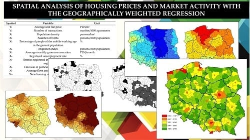
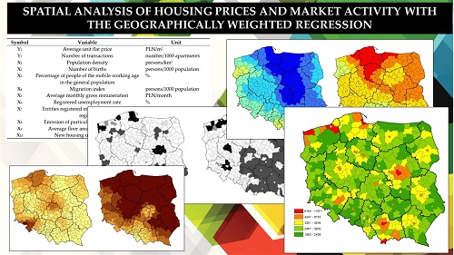
Figure 1. Average price of 1 m2 and number of flats sold in 2018 in each county in Poland. Source: own research based on GUS (Central Statistical Office) data.
Ijgi 09 00380 g001
Figure 2. Local and global statistics of Moran’s I. Source: own research based on GUS data. Source: own research.
Ijgi 09 00380 g002
Figure 3. Spatial distribution of the parameters at local variables in the MGWR1 model (standardised variable values were used for estimation). Source: own research.
Ijgi 09 00380 g003
Figure 4. Spatial distribution of statistic t for coefficients at local variables in the MGWR1 model. Source: own research.
Ijgi 09 00380 g004
Figure 5. Spatial distribution of the parameters at local variables in the MGWR2 model (standardised variable values were used for estimation). Source: own research.
Ijgi 09 00380 g005
Figure 6. Spatial distribution of statistic t for coefficients at local variables in the MGWR2 model. Source: own research.
Ijgi 09 00380 g006
Figure 7. Local R2 in the Geographically Weighted Regression (GWR) models. Source: own research.
Ijgi 09 00380 g007
Table 1. Variables taken for analysis.
SymbolVariableUnit
Y1Average unit flat pricePLN/m2 (New Polish Zloty/m2)
Y2Number of transactionsnumber/1000 apartments
X1Population densitypersons/km2
X2Number of birthspersons/1000 population
X3Percentage of people of the mobile working age in the general population%
X4Migration indexpersons/1000 population
X5Average monthly gross remunerationPLN/month
X6Registered unemployment rate%
X7Entities registered in the business entities registernumber/1000 population
X8Emission of particulate pollutants PM10 (a mixture of airborne particles with a diameter of not more than 10 μm)t/km2
X9Average floor area of a housing unitm2
X10New housing units completedunits/1000 population
Table 2. Main descriptive statistics of the variables taken for analysis. SD = standard deviation, Coef. of variation = coefficient. of variation.
VariableMinimumAverageMedianMaximumSDCoef. of Variation
Y11063.0003120.5872887.75011,671.2501099.3010.352
Y20.0709.3327.71142.2867.4610.799
X119.000369.46390.5003757.000655.1361.773
X2−10.570−1.122−1.2459.4202.616−2.332
X355.80061.05361.20064.4001.3330.022
X4−79.956−12.407−19.726269.20440.243−3.243
X53183.3404142.1384017.1708121.080561.9830.136
X61.2007.7966.95024.3004.0590.521
X74.4738.8938.40821.0062.3050.259
X80.0000.4090.03019.4701.3743.358
X922.23327.69527.30743.1003.1260.113
X100.5993.5482.94816.9382.5200.710
Table 3. Parameters of OLS (ordinary least squares) models with response variables Y1 and Y2.
Model OLS1: Explained Variable Y1Model OLS2: Explained Variable Y2
VariableEstimateStandard Errorp-ValueEstimateStandard Errorp-Value
Intercept5274.5002412.2810.0299.53816.1580.555
X10.1700.074<0.0010.003<0.001<0.001
X262.59118.8420.002−0.5530.126<0.001
X3−113.47336.894<0.0010.0720.2470.770
X4−5.1481.431<0.001<0.0010.0090.973
X50.2520.073<0.0010.001<0.0010.001
X6−16.62711.4200.146−0.0920.0760.228
X7201.58921.534<0.0010.8620.144<0.001
X8−26.22128.7380.362−0.0400.1920.840
X961.12615.960<0.001−0.9360.107<0.001
X1092.56824.343<0.0011.7300.163<0.001
R2 = 0.627, adjusted R2 = 0.615, F = 61.95, p-value < 0.001R2 = 0.636, adjusted R2 = 0.626, F = 64.58, p-value < 0.001
Table 4. General characteristics of Geographically Weighted Regression (GWR) model parameters with response variables Y1 and Y2.
Model GWR1: Explained Variable Y1Model GWR2: Explained Variable Y2
VariableMinMeanMaxMinMeanMax
Intercept−29,273.6405791.51319,715.073−32.14722.05094.227
X1−0.4570.1791.8570.0010.0030.009
X2−106.88027.134260.713−1.098−0.2681.207
X3−392.461100.259337.890−1.292−0.1341.796
X4−11.007−2.26410.934−0.0110.0040.073
X50.0630.3090.881−0.0020.0010.006
X6−95.599−39.94440.515−0.355−0.0300.636
X7−45.708154.211416.206−0.7310.3322.068
X8−514.866−30.6091491.609−3.661−0.0675.925
X9−62.21129.364306.800−1.666−0.6061.763
X10−152.25991.005250.9840.6251.3671.580
Local R20.6730.8240.9290.6780.7650.873
Bandwidth208.177 km264.770 km
Table 5. Results of the variability test for GWR model coefficients.
VariableModel GWR1Model GWR2
Difference (AICc)Difference (AICc)
Intercept−1343.857−2140.382
X14.2266.769
X2−7.7463.604
X3−971.042−1654.359
X41.7912.849
X5−73.429−143.213
X62.628−3.382
X7−19.018−85.209
X8−5.470−1.719
X9−190.189−848.640
X10−9.038−20.806
Table 6. Results of the MGWR1 (mixed geographically weighted regression) model parameter estimation.
Global Variables (Fixed).Local Variables
VariableEstimateStandard Errorp-ValueVariableMinMeanMax
X10.0580.0710.413Intercept−3554.8288723.07821,493.044
X4−1.6701.3170.223X2−102.21930.120235.182
X6−27.03811.897<0.001X3−367.237−149.30132.045
R2 = 0.825, Adjusted R2 = 0.872
Loglik = 5737.308 (likehood function logarithm)
AIC = 5858.230, AICc = 5881.561 (Akaike criterion)
BIC = 6096.457 (Bayesian information criterion)
X50.0470.3240.936
X732.429168.906405.211
X8−256.046−31.748308.190
X9−54.45021.286156.876
X10−50.59092.550189.093
Table 7. Results of the MGWR2 model parameter estimation.
Global Variables (Fixed)Local Variables
VariableEstimateStandard Errorp-ValueVariableMinMeanMax
X12.8230.309<0.001Intercept5.3288.69012.058
X2−0.6970.2940.018X3−1.593−0.2991.071
X40.5960.3560.094X5−0.5410.8942.121
X6−0.2090.0110.476
R2 = 0.805, Adjusted R2 = 0.767
Loglik = 1982.374 (likehood function logarithm)
AIC = 2083.313, AICc = 2099.127 (Akaike criterion)
BIC = 2282.172 (Bayesian information criterion)
X7−0.4100.3431.080
X8−1.269−0.0100.897
X9−1.235−0.6060.012
X100.6071.4212.100
Table 8. Basic diagnostic statistics of OLS, GWR and MGWR models.
OLS1GWR1MGWR1OLS2GWR2MGWR2
Standard Error670.776463.981459.5054.4963.2133.252
R20.6270.8210.8250.6330.8140.809
Adjusted R20.6150.7750.7820.6220.7660.769
logLik6024.8045744.6745737.3082220.8881965.6111974.595
AIC6048.8045868.6915858.2302244.8882089.6272083.103
AICc6049.6545893.3425881.5612245.7382114.2782101.565
BIC6096.0866113.0156069.4572292.1702333.9512296.873

