Assessment and Quantification of the Accuracy of Low- and High-Resolution Remote Sensing Data for Shoreline Monitoring


Abstract
:1. Introduction
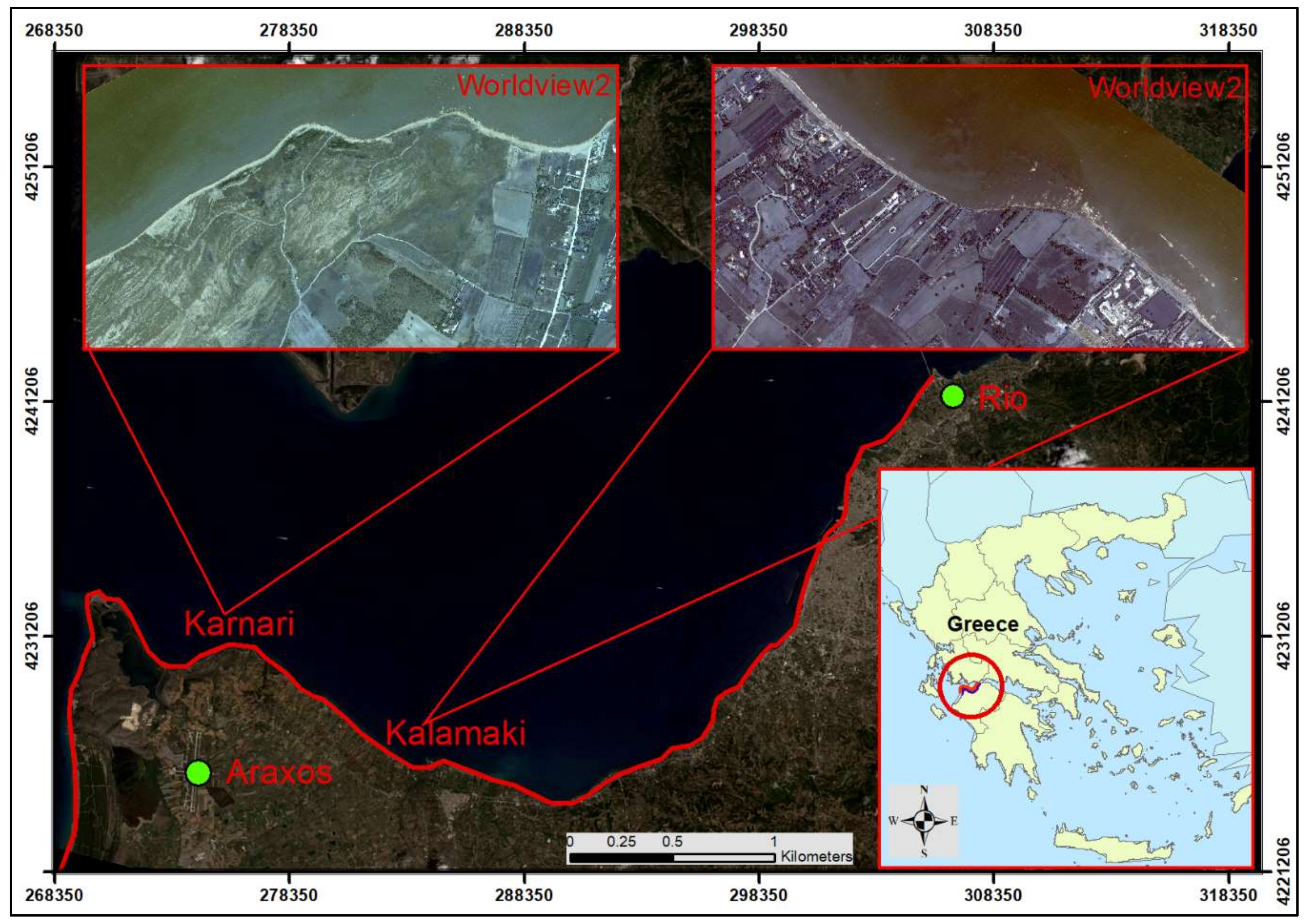
2. Study Area
3. Materials and Methods
3.1. Materials
3.2. Methods
3.2.1. Shoreline Digitizing and DSAS Procedure
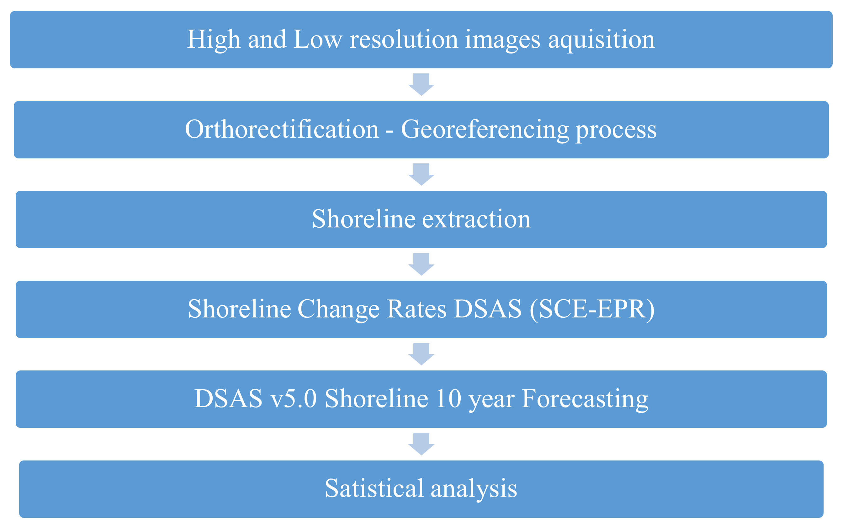
3.2.2. Procedure
4. Results
4.1. First Goal Results (Accuracy)
4.2. Second Goal Results (Forecasting)
5. Discussion
6. Conclusions
Author Contributions
Funding
Acknowledgments
Conflicts of Interest
References
- Cracknell, A.P. The development of remote sensing in the last 40 years. Int. J. Remote Sens. 2018, 39, 8387–8427. [Google Scholar] [CrossRef] [Green Version]
- Bird, E.C.F. Beach Management; John Wiley & Son Ltd.: Chichester, UK, 1996; Volume 5. [Google Scholar]
- Alexandrakis, G.; Manasakis, C.; Kampanis, N.A. Valuating the effects of beach erosion to tourism revenue. A management perspective. Ocean Coast. Manag. 2015, 111, 1–11. [Google Scholar] [CrossRef]
- Valderrama-Landeros, L.; Flores-de-Santiago, F. Assessing coastal erosion and accretion trends along two contrasting subtropical rivers based on remote sensing data. Ocean Coast. Manag. 2019, 169, 58–67. [Google Scholar] [CrossRef]
- Hashmi, S.G.M.D.; Ahmad, S. GIS-Based Analysis and Modeling of Coastline Erosion and Accretion along the Coast of Sindh Pakistan. J. Coast. Zone Manag. 2018, 21, 6–9. [Google Scholar] [CrossRef]
- Ahmed, A.; Drake, F.; Nawaz, R.; Woulds, C. Where is the coast? Monitoring coastal land dynamics in Bangladesh: An integrated management approach using GIS and remote sensing techniques. Ocean Coast. Manag. 2018, 151, 10–24. [Google Scholar] [CrossRef]
- Natesan, U.; Parthasarathy, A.; Vishnunath, R.; Kumar GE, J.; Ferrer, V.A. Monitoring Longterm Shoreline Changes along Tamil Nadu, India Using Geospatial Techniques. Aquat. Procedia 2015, 4, 325–332. [Google Scholar] [CrossRef]
- Salghuna, N.N.; Bharathvaj, A.S. Shoreline Change Analysis for Northern Part of the Coromandel Coast. Aquat. Procedia 2015, 4, 317–324. [Google Scholar] [CrossRef]
- Wenyu, L.; Peng, G. Continuous monitoring of coastline dynamics in western Florida with a 30-year time series of Landsat imagery. Remote Sens. Environ. 2016, 179, 196–209. [Google Scholar] [CrossRef]
- Pardo-Pascual, J.E.; Almonacid-Caballer, J.; Ruiz, L.A.; Palomar-Vázquez, J. Automatic extraction of shorelines from Landsat TM and ETM+ multi-temporal images with subpixel precision. Remote Sens. Environ. 2012, 123, 1–11. [Google Scholar] [CrossRef] [Green Version]
- Kankara, R.S.; Selvan, S.C.; Markose, V.J.; Rajan, B.; Arockiaraj, S. Estimation of Long and Short Term Shoreline Changes Along Andhra Pradesh Coast Using Remote Sensing and GIS Techniques. Procedia Eng. 2015, 116, 855–862. [Google Scholar] [CrossRef] [Green Version]
- Chen, C.; Fu, J.; Zhang, S.; Zhao, X. Coastline information extraction based on the tasseled cap transformation of Landsat-8 OLI images. Estuar. Coast. Shelf Sci. 2019, 217, 281–291. [Google Scholar] [CrossRef]
- Feyisa, G.L.; Meilby, H.; Fensholt, R.; Proud, S.R. Automated Water Extraction Index: A new technique for surface water mapping using Landsat imagery. Remote Sens. Environ. 2014, 140, 23–35. [Google Scholar] [CrossRef]
- Esmail, M.; Mahmod WElham Fath, H. Assessment and prediction of shoreline change using multi-temporal satellite images and statistics: Case study of Damietta coast, Egypt. Appl. Ocean Res. 2019, 82, 274–282. [Google Scholar] [CrossRef]
- Joevivek, V.; Saravanan, S.; Chandrasekar, N. Assessing the shoreline trend changes in Southern tip of India. J. Coast. Conserv. 2018, 23, 283–292. [Google Scholar] [CrossRef]
- Song, Y.; Liu, F.; Feng, L.; Yue, L. Automatic Semi-Global Artificial Shoreline Subpixel Localization Algorithm for Landsat Imagery. Remote Sens. 2019, 11, 1779. [Google Scholar] [CrossRef] [Green Version]
- Zed, A.A.; Soliman, M.R.; Yassin, A.A. Evaluation of using satellite image in detecting long term shoreline change along El-Arish coastal zone, Egypt. Alex. Eng. J. 2018, 57, 2687–2702. [Google Scholar] [CrossRef]
- Cenci, L.; Disperati, L.; Sousa, L.; Phillips, M.; Alves, F. Geomatics for Integrated Coastal Zone Management: Multitemporal shoreline analysis and future regional perspective for the Portuguese Central Region. J. Coast. Res. 2013, 5, 1349–1354. [Google Scholar] [CrossRef] [Green Version]
- Dewi, R. Monitoring long-term shoreline changes along the coast of Semarang. In IOP Conference Series: Earth and Environmental Science; IOP Publishing Ltd.: Bristol, UK, 2019; Volume 284, p. 012035. [Google Scholar] [CrossRef]
- Konko, Y.; Bagaram, M.; Julien FAkpamou, K.; Kokou, K. Multitemporal Analysis of Coastal Erosion Based on Multisource Satellite Images in the South of the Mono Transboundary Biosphere Reserve in Togo (West Africa). Open Access Libr. J. 2018, 5, e4526. [Google Scholar] [CrossRef]
- Rakesh, B.; Ramkrishna, M. Quantitative analysis of erosion and accretion (1975–2017) using DSAS—A study on Indian Sundarbans. Reg. Stud. Mar. Sci. 2019, 28, 100583. [Google Scholar] [CrossRef]
- Thakur, S.; Dey, D.; Das, P.; Ghosh, P.; De, T. Shoreline Change Detection Using Remote Sensing in the Bakkhali Coastal Region, West Bengal, India. Indian J. Geosci. 2018, 71, 611–626. [Google Scholar]
- Liu, Q.; Trinder, J. Sub-Pixel Technique for Time Series Analysis of Shoreline Changes Based on Multispectral Satellite Imagery. IntechOpen 2018. [Google Scholar] [CrossRef] [Green Version]
- Dewi, R.; Bijker, W.; Stein, A.; Marfai, M.A. Transferability and Upscaling of Fuzzy Classification for Shoreline Change over 30 Years. Remote Sens. 2018, 10, 1377. [Google Scholar] [CrossRef] [Green Version]
- Manjulavani, K.; Supriya, V.M.; Suhrullekha, M.; Harish, B. Detection of shoreline change using geo-spatial techniques along the coast between Kanyakumari and Tuticorin. In Proceedings of the 2017 IEEE International Conference on Power, Control, Signals and Instrumentation Engineering (ICPCSI), Chennai, India, 21–22 September 2017; pp. 2822–2825. [Google Scholar] [CrossRef]
- Shenbagaraj, N.; Mani, N.D.; Muthukumar, M. Isodata classification technique to assess the shoreline changes of Kolachel to Kayalpattanam coast. Int. J. Eng. Res. Technol. 2014, 3, 311–314. [Google Scholar]
- Addo, K.A.; Quashigah, K.S.; Kufogbe, K.S. Quantitative analysis of shoreline change using medium resolution satellite imagery in Keta, Ghana. Mar. Sci. 2011, 1, 1–9. [Google Scholar] [CrossRef] [Green Version]
- Nassar, K.; Mahmod, W.E.; Fath, H.; Masria, A.; Nadaoka, K.; Negm, A. Shoreline change detection using DSAS technique: Case of North Sinai coast. Egypt. Mar. Georesources Geotechnol. 2019, 37, 81–95. [Google Scholar] [CrossRef]
- Kawakubo, F.S.; Morato, R.G.; Nader, R.S.; Luchiari, A. Mapping changes in coastline geomorphic features using Landsat TM and ETM+ imagery: Examples in southeastern Brazil. Int. J. Remote Sens. 2011, 32, 2547–2562. [Google Scholar] [CrossRef]
- Vanderstraete, T.; Goossens, R.; Ghabour, T. The use of multi-temporal Landsat images for the change detection of the coastal zone near Hurghada, Egypt. Int. J. Remote Sens. 2006, 27, 3645–3655. [Google Scholar] [CrossRef]
- Mitra, S.; Mitra, D.; Abhisek, S. Performance testing of selected automated coastline detection techniques applied on multispectral satellite imageries. Earth Sci. Inform. 2017, 10, 321–330. [Google Scholar] [CrossRef]
- Liu, Q.; Trinder, J.C.; Turner, I.L. Automatic super-resolution shoreline change monitoring using Landsat archival data: A case study at Narrabeen-Collaroy Beach, Australia. J. Appl. Remote Sens. 2017, 11, 016036. [Google Scholar] [CrossRef]
- Xu, N. Detecting Coastline Change with All Available Landsat Data over 1986–2015: A Case Study for the State of Texas, USA. Atmosphere 2018, 9, 107. [Google Scholar] [CrossRef] [Green Version]
- Viaña-Borja, S.P.; Ortega-Sánchez, M. Automatic Methodology to Detect the Coastline from Landsat Images with a New Water Index Assessed on Three Different Spanish Mediterranean Deltas. Remote Sens. 2019, 11, 2186. [Google Scholar] [CrossRef] [Green Version]
- Yulianto, F.S.; Maulana, T.; Khomarudin, M.R. Analysis of the dynamics of coastal landform change based on the integration of remote sensing and gis techniques: Implications for tidal flooding impact in pekalongan, central java, Indonesia. Quaest. Geogr. 2019, 38, 17–29. [Google Scholar] [CrossRef] [Green Version]
- Marfai, M.A.; Almohammad, H.; Dey, S.; Susanto, B.; King, L. Coastal dynamic and shoreline mapping: Multi-sources spatial data analysis in Semarang Indonesia. Environ. Monit. Assess. 2008, 142, 297–308. [Google Scholar] [CrossRef] [PubMed]
- Guariglia, A.; Buonamassa, A.; Losurdo, A.; Saladino, R.; Trivigno, M.L.; Zaccagnino, A.; Colangelo, A. A multisource approach for coastline mapping and identification of shoreline changes. Ann. Geophys. 2009, 49. [Google Scholar] [CrossRef]
- Li, X.; Damen, M.C.J. Coastline change detection with satellite remote sensing for environmental management of the Pearl River Estuary, China. J. Mar. Syst. 2010, 82, S54–S61. [Google Scholar] [CrossRef]
- Bergillos, R.J.; Ortega-Sánchez, M. Assessing and mitigating the landscape effects of river damming on the Guadalfeo River delta, southern Spain. Landsc. Urban Plan. 2017, 165, 117–129. [Google Scholar] [CrossRef]
- Zhao, B.; Guo, H.; Yan, Y.; Wang, Q.; Li, B. A simple waterline approach for tidelands using multi-temporal satellite images: A case study in the Yangtze Delta. Estuar. Coast. Shelf Sci. 2008, 77, 134–142. [Google Scholar] [CrossRef]
- Ghosh, M.K.; Kumar, L.; Roy, C. Monitoring the coastline change of Hatiya Island in Bangladesh using remote sensing techniques. ISPRS J. Photogramm. Remote Sens. 2015, 101, 137–144. [Google Scholar] [CrossRef]
- Kuleli, T. Quantitative analysis of shoreline changes at the Mediterranean Coast in Turkey. Environ. Monit. Assess. 2010, 167, 387–397. [Google Scholar] [CrossRef]
- Wang, X.; Liu, Y.; Ling, F.; Liu, Y.; Fang, F. Spatio-temporal change detection of ningbo coastline using Landsat time-deries images during 1976–2015. ISPRS Int. J. Geo. Inf. 2017, 6, 68. [Google Scholar] [CrossRef] [Green Version]
- Kakonas, A.; Karymbalis, E.; Chalkias, C.; Evelpidou, N. Flood hazard assessment of the Kerinitis River catchment, North Peloponnese, Greece. In Proceedings of the 15th International Congress of the Geological Society of Greece, Athens, Greece, 22—24 May 2019. [Google Scholar]
- Ferentinos, G.; Brooks, M.; Doutsos, T. Quaternary tectonics in the Gulf of Patras, western Greece. J. Struct. Geol. 1985, 7, 713–717. [Google Scholar] [CrossRef]
- Fourniotis, N.T.; Horsch, G.M. Baroclinic circulation in the Gulf of Patras (Greece). Ocean Eng. 2015, 104, 238–248. [Google Scholar] [CrossRef]
- Digital Globe®, White Paper: The Benefits of the 8 Spectral Bands of WorldView-2. 2010. Available online: http://www.satimagingcorp.com/media/pdf/WorldView-2_8-Band_Applications_Whitepaper.pdf (accessed on 20 April 2020).
- Xu, H. Modification of Normalised Difference Water Index (NDWI) to enhance open water features in remotely sensed imagery. Int. J. Remote Sens. 2006, 27, 3025–3033. [Google Scholar] [CrossRef]
- Rasuly, A.; Naghdifar, R.; Rasoli, M. Monitoring of Caspian Sea Coastline Changes Using Object-Oriented Techniques. Procedia Environ. Sci. 2010, 2, 416–426. [Google Scholar] [CrossRef] [Green Version]
- Thieler, E.R.; Himmelstoss, E.A.; Zichichi, J.L.; Ergul, A. Digital Shoreline Analysis System (DSAS) Version 4.4, An ArcGIS Extension for Calculating Shoreline Change. US Geological Survey Open-File Report 2017, 2008-1278. Available online: https://pubs.er.usgs.gov/publication/ofr20081278/# (accessed on 17 April 2020).
- Himmelstoss, E.A.; Henderson, R.E.; Kratzmann, M.G.; Farris, A.S. Digital Shoreline Analysis System (DSAS) Version 5.0 User Guide; Open-File Report 2018-1179; U.S. Geological Survey: Woods Hole, MA, USA, 2018. [CrossRef] [Green Version]
- Long, J.W.; Plant, N.G. Extended Kalman Filter framework for forecasting shoreline evolution. Geophys. Res. Lett. 2012, 39, 1–6. [Google Scholar] [CrossRef]
- NASA. Landsat 7 science Data Users Handbook. 2006. Available online: https://landsat.gsfc.nasa.gov/wp-content/uploads/2016/08/Landsat7_Handbook.pdf (accessed on 14 April 2020).
- Almonacid, C.J.; Sánchez, G.E.; Pardo PJ, E.; Balaguer BA, A.; Palomar, V.J. Evaluation of annual mean shoreline position deduced from Landsat imagery as a mid-term coastal evolution indicator. Mar. Geol. 2016, 372, 79–88. [Google Scholar] [CrossRef]
- Pardo-Pascual, J.E.; Sánchez-García, E.; Almonacid-Caballer, J.; Palomar-Vázquez, J.M.; Priego de los Santos, E.; Fernández-Sarría, A.; Balaguer-Beser, Á. Assessing the Accuracy of Automatically Extracted Shorelines on Microtidal Beaches from Landsat 7, Landsat 8 and Sentinel-2 Imagery. Remote Sens. 2018, 10, 326. [Google Scholar] [CrossRef] [Green Version]
- Cenci, L.; Disperati, L.; Persichillo, M.G.; Oliveira, E.R.; Alves, F.L.; Phillips, M. Integrating remote sensing and GIS techniques for monitoring and modeling shoreline evolution to support coastal risk management. GISci. Remote Sens. 2017, 55, 355–375. [Google Scholar] [CrossRef]
- Louati, M.; Saïdi, H.; Zargouni, F. Shoreline change assessment using remote sensing and GIS techniques: A case study of the Medjerda delta coast, Tunisia. Arab. J. Geosci. 2015, 8, 4239–4255. [Google Scholar] [CrossRef]
- Kermani, S.; Boutiba, M.; Guendouz, M.; Guettouche, M.S.; Khelfani, D. Detection and analysis of shoreline changes using geospatial tools and automatic computation: Case of jijelian sandy coast (East Algeria). Ocean Coast. Manag. 2016, 132, 46–58. [Google Scholar] [CrossRef]
- Nikolakopoulos, K.; Kyriou, A.; Koukouvelas, I.; Zygouri, V.; Apostolopoulos, D. Combination of Aerial, Satellite, and UAV Photogrammetry for Mapping the Diachronic Coastline Evolution: The Case of Lefkada Island. ISPRS Int. J. Geo Inf. 2019, 8, 489. [Google Scholar] [CrossRef] [Green Version]


| Year | Data Type | Source | Reference System | Number of Photos | Spatial Resolution | Datasets |
|---|---|---|---|---|---|---|
| 1945 | Orthomosaic | National Greek Cadastre and Mapping Agency | Hellenic Geodetic Reference System of 1987 (Greek Grid) | 1 | 1 m | No further processing |
| 2008 | Orthomosaic | National Greek Cadastre and Mapping Agency | Hellenic Geodetic Reference System of 1987 (Greek Grid) | 1 | 1 m | No further processing |
| 1996 | Orthomosaic | Ministry of Rural Development and Food | Hellenic Geodetic Reference System of 1987 (Greek Grid) | 1 | 1 m | No further processing |
| 1973 | Declassified satellite imagery | USGS | No reference system | 1 | 4 m | Orthorectified using LPS Suite |
| 2000–2008 | (Landsat 7 (ETM+)) | USGS | Universal Transverse Mercator Zone 34 (EPSG 32634) | 1 | 30 m | Georeferenced to Hellenic Geodetic Reference System of 1987 (Greek Grid) |
| 2018 | (Landsat 8/OLI) | USGS | Universal Transverse Mercator Zone 34 (EPSG 32634) | 1 | 30 m | Georeferenced to Hellenic Geodetic Reference System of 1987 (Greek Grid) |
| 2018 | Worldview-2 | Digital Globe | Universal Transverse Mercator Zone 34 (EPSG 32634) | 1 | 0.50 m | Orthorectified using LPS Suite |
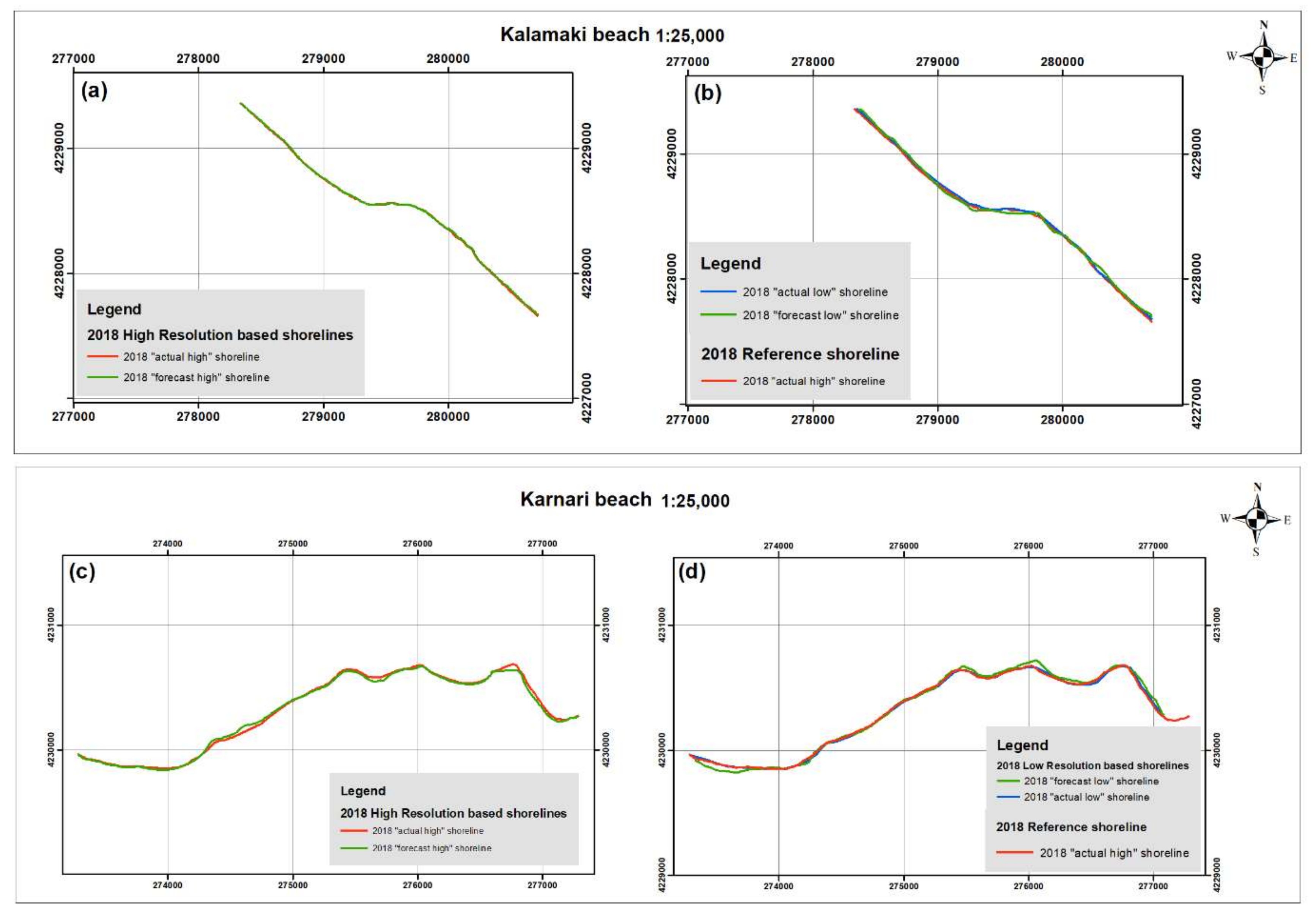
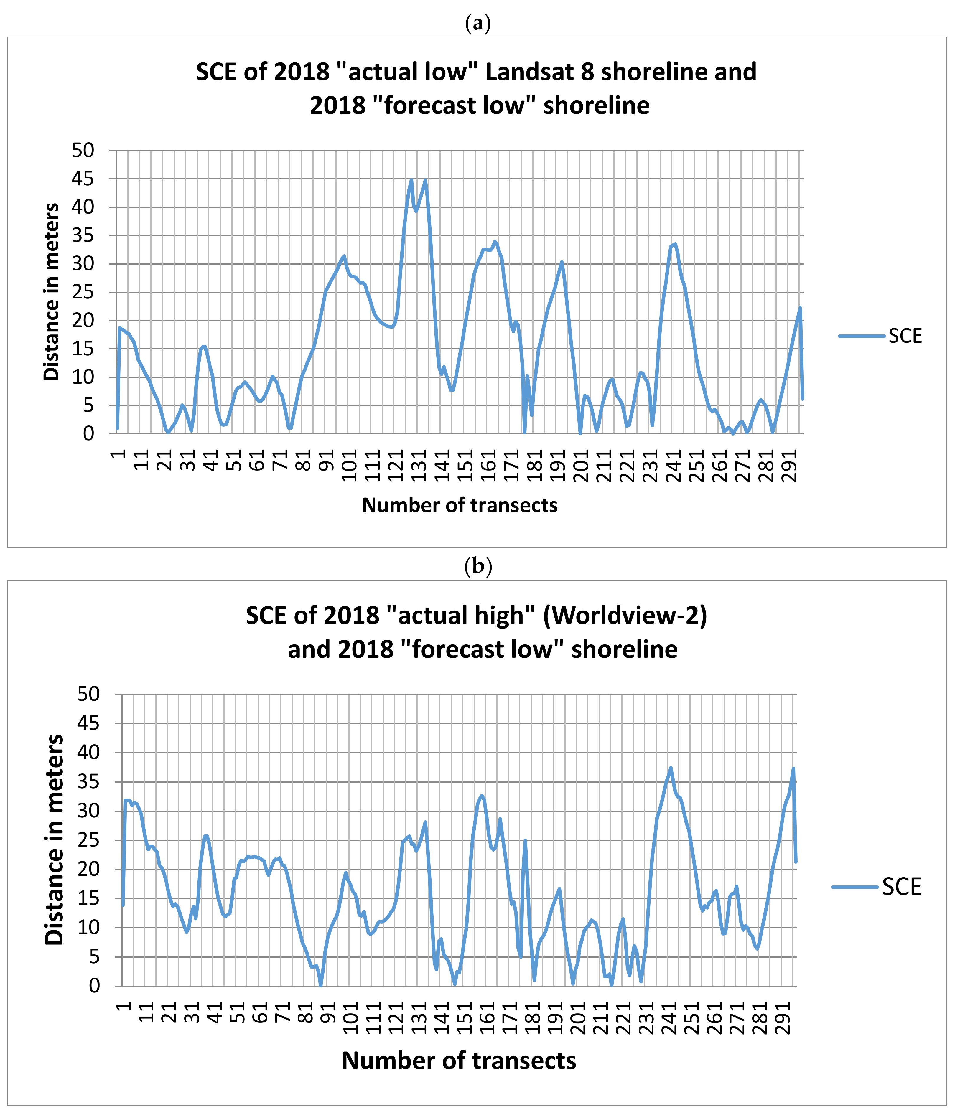
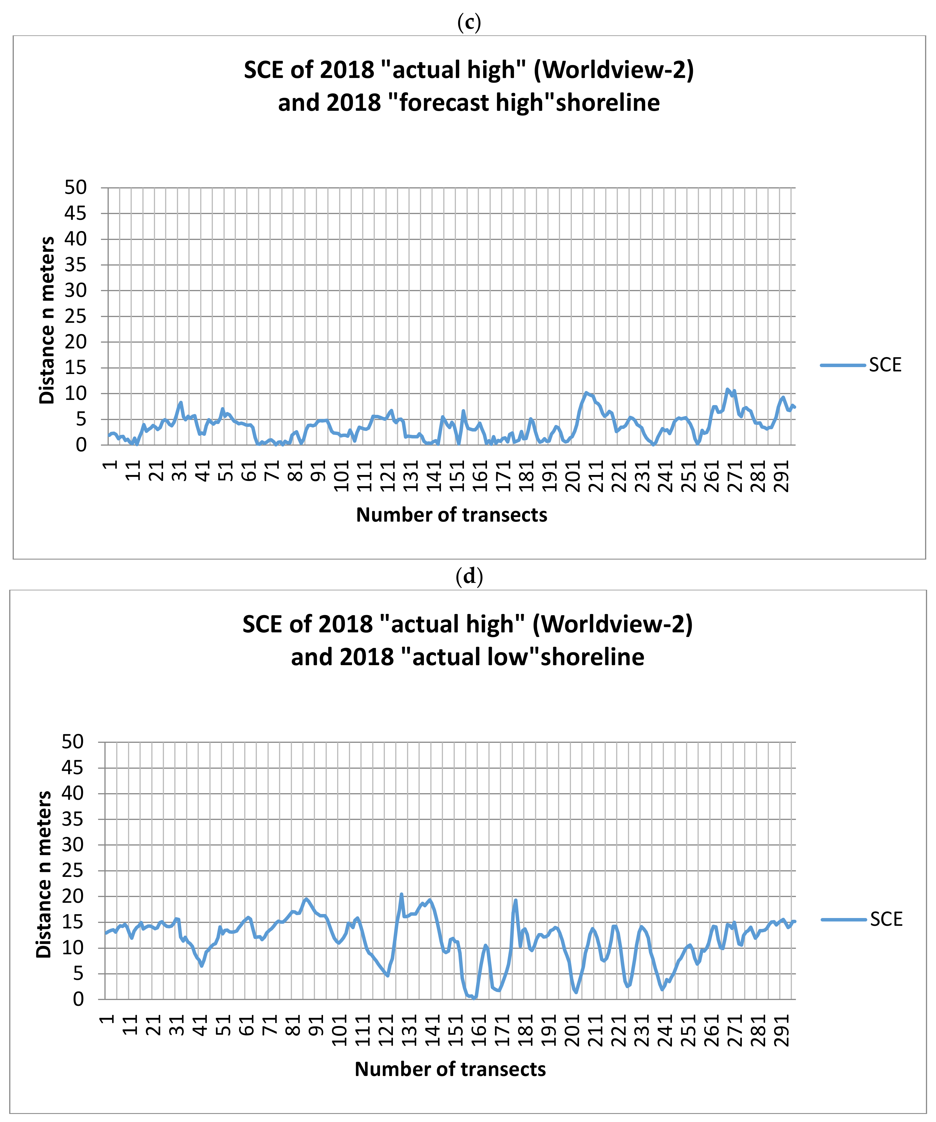
| Kalamaki Beach | |||||
|---|---|---|---|---|---|
| 2018 Shoreline Overlapping | Figures | Min | Max | Mean | Standard Deviation (σ) |
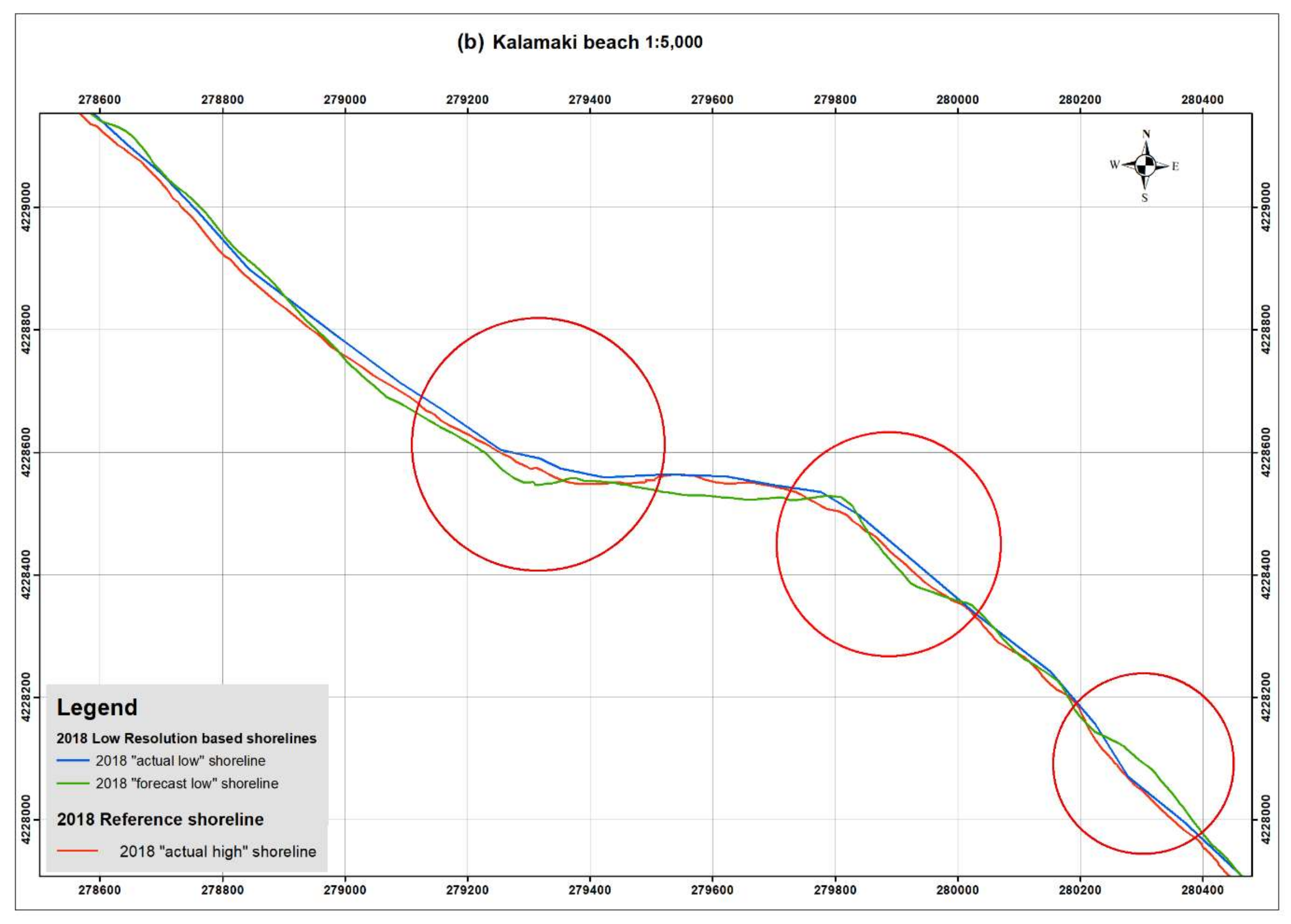
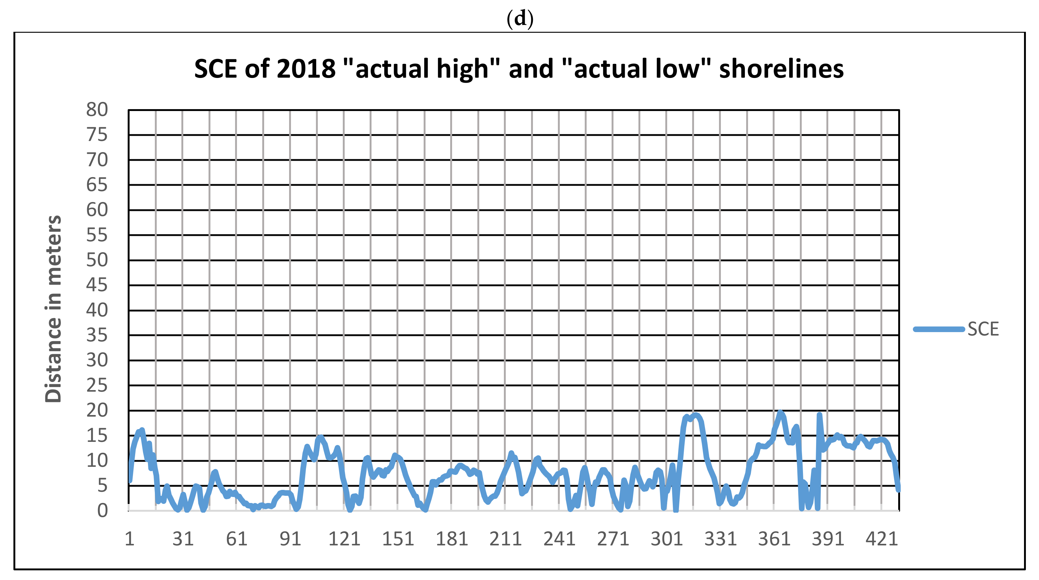
| “actual low” and “forecasted low” | Figure 9a | 0.00 | 44.81 | 14.38 | 11.05 |
| “actual high” and “forecasted low” | Figure 9b | 0.09 | 37.42 | 15.94 | 8.87 |
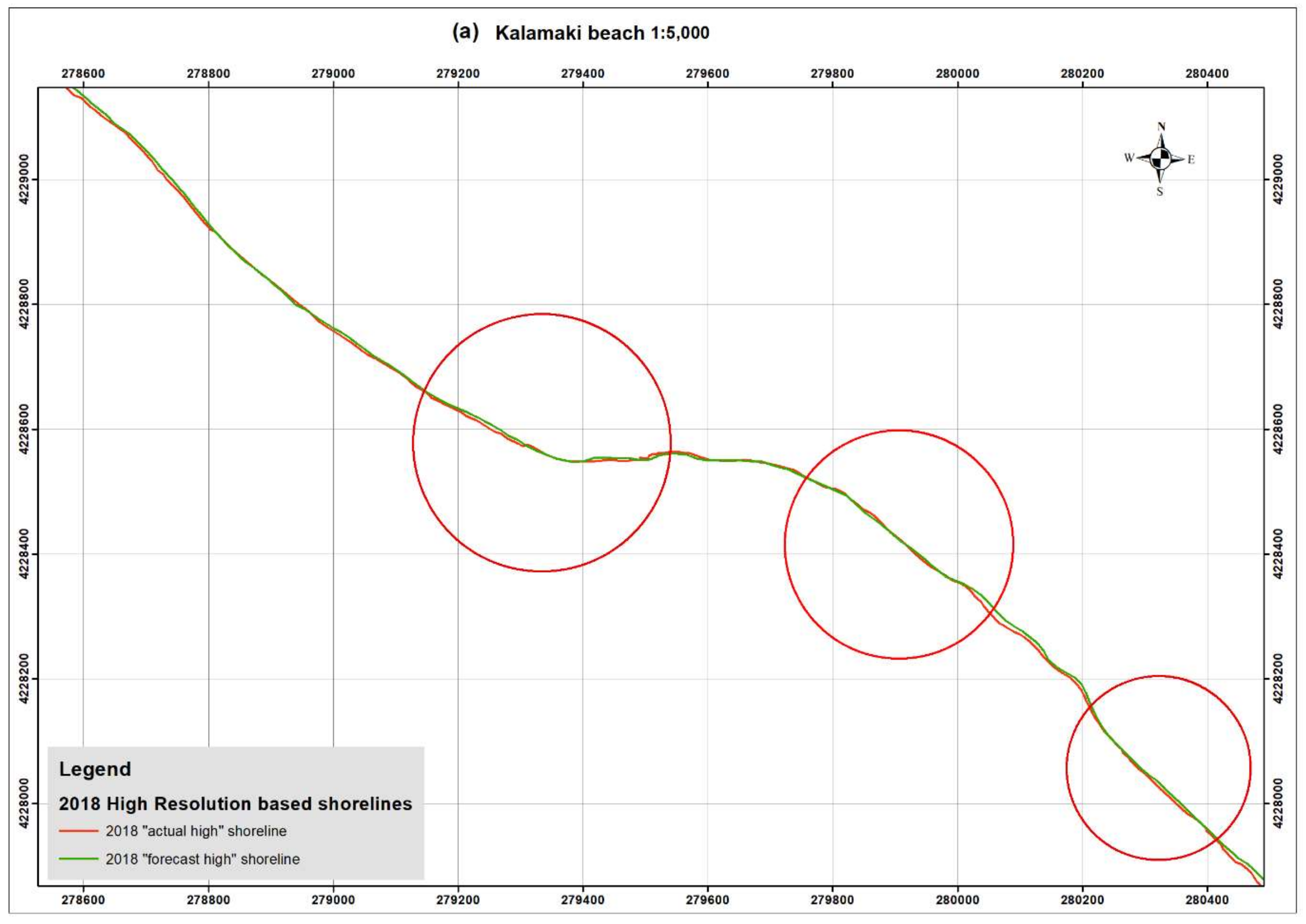
| “actual high” and “forecasted high” | Figure 9c | 0.04 | 10.84 | 3.60 | 2.39 |
| “actual high” and “ actual low” | Figure 9d | 0.20 | 20.46 | 11.61 | 4.28 |
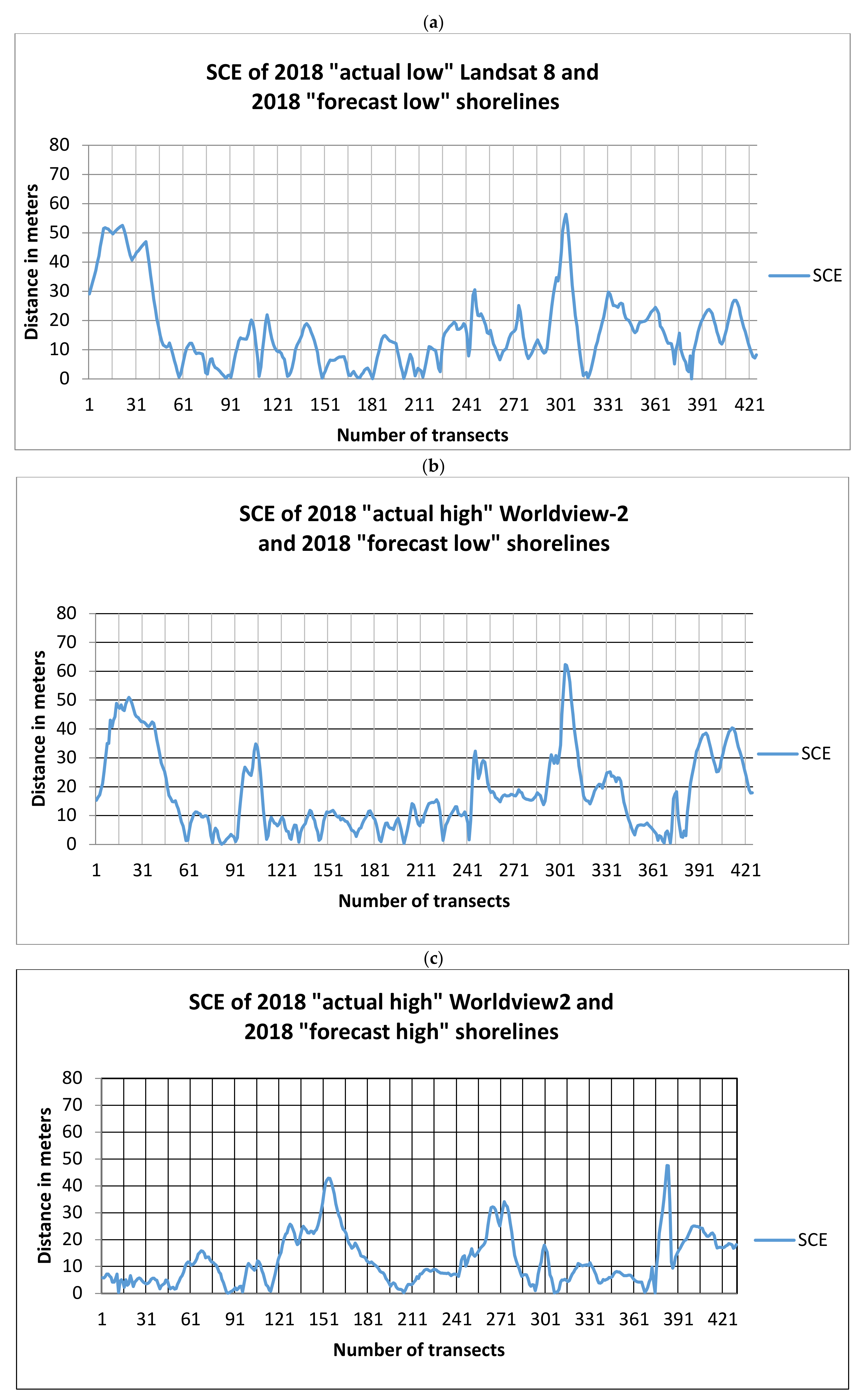
| Karnari Beach | |||||
|---|---|---|---|---|---|
| 2018 Shoreline Overlapping | Figures | Min | Max | Mean | Standard Deviation (σ) |
| “actual low” and “forecasted low” | Figure 10a | 0.01 | 56.35 | 16.17 | 12.89 |
| “actual high” and “forecasted low” | Figure 10b | 0.08 | 62.31 | 17.47 | 13.47 |
| “actual high” and “forecasted high” | Figure 10c | 0.03 | 47.63 | 12.17 | 9.49 |
| “actual high” and “ actual low” | Figure 10d | 0.01 | 19.66 | 7.37 | 4.90 |
| Kalamaki Beach | |||||
|---|---|---|---|---|---|
| Data Resolution | Figures | Min | Max | Mean | Standard Deviation (σ) |
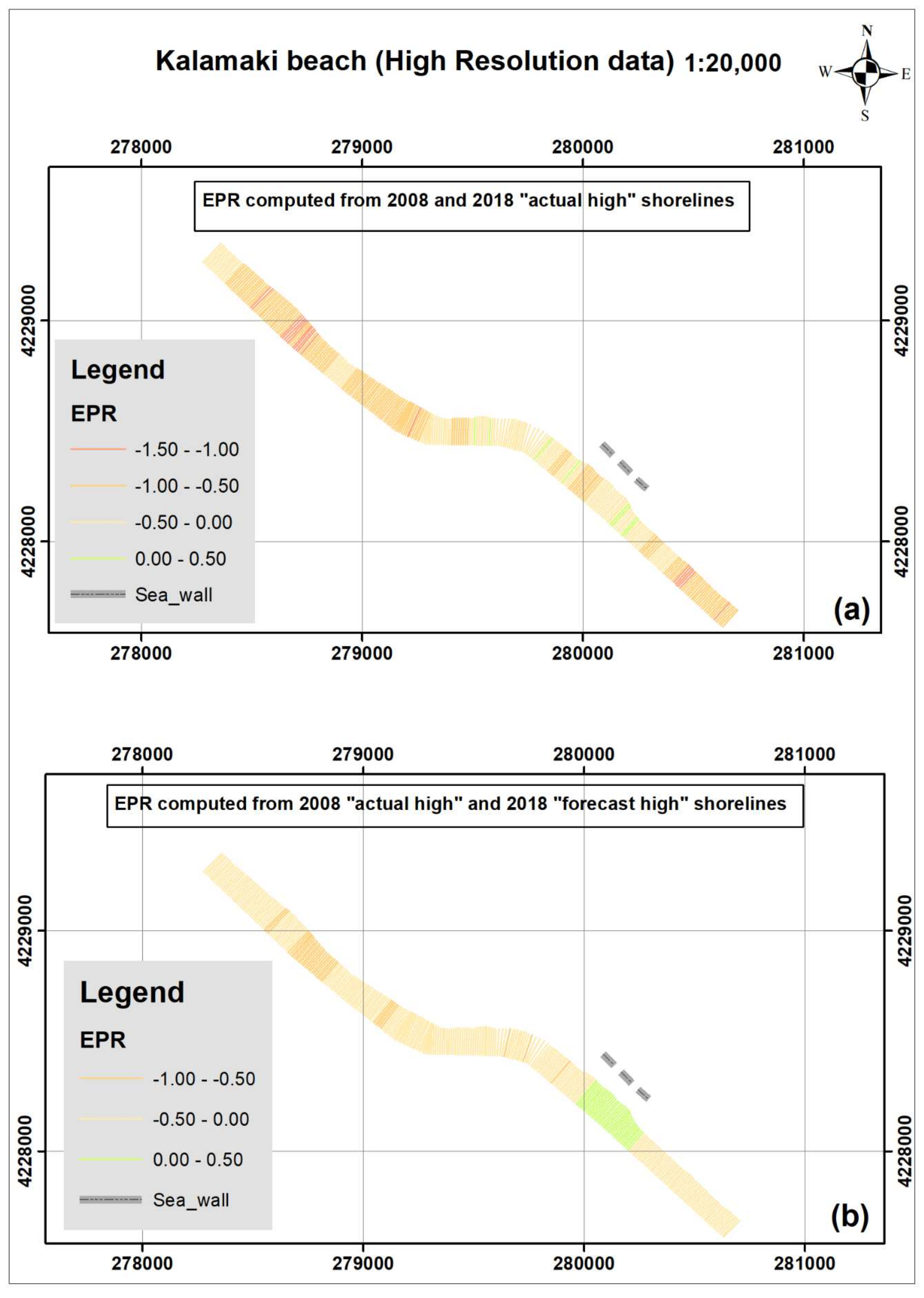
| 2008 and 2018 “actual high” | Figure 11a | −1.26 | 0.20 | −0.54 | 0.31 |
| 2008 “actual high” and 2018 “forecasted high” | Figure 11b | −0.64 | 0.51 | −0.25 | 0.23 |
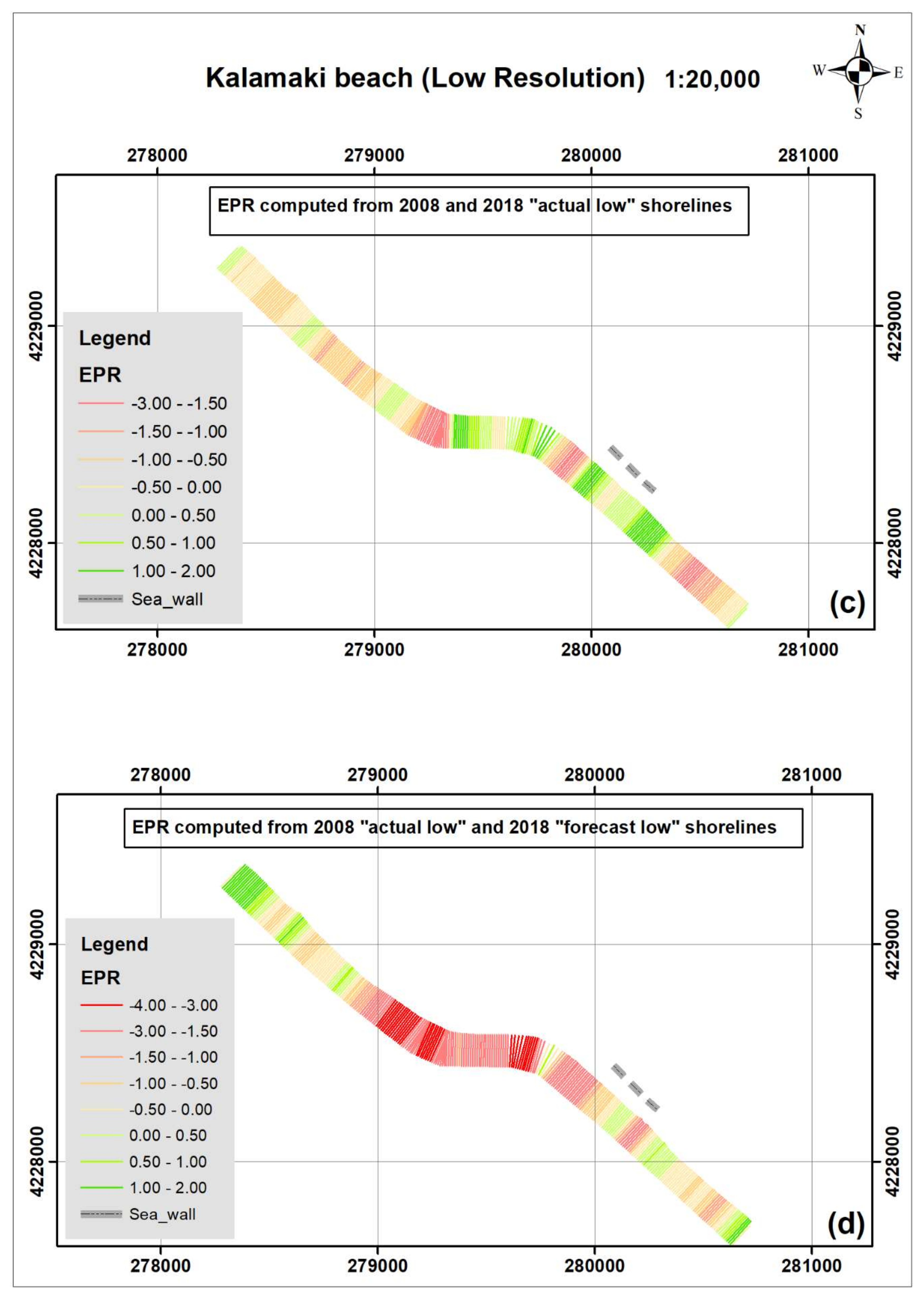
| 2008 and 2018 “actual low” | Figure 11c | −3.05 | 1.84 | −0.32 | 0.95 |
| 2008 “actual low” and 2018 “forecasted low” | Figure 11d | −3.73 | 1.89 | −1.00 | 1.40 |
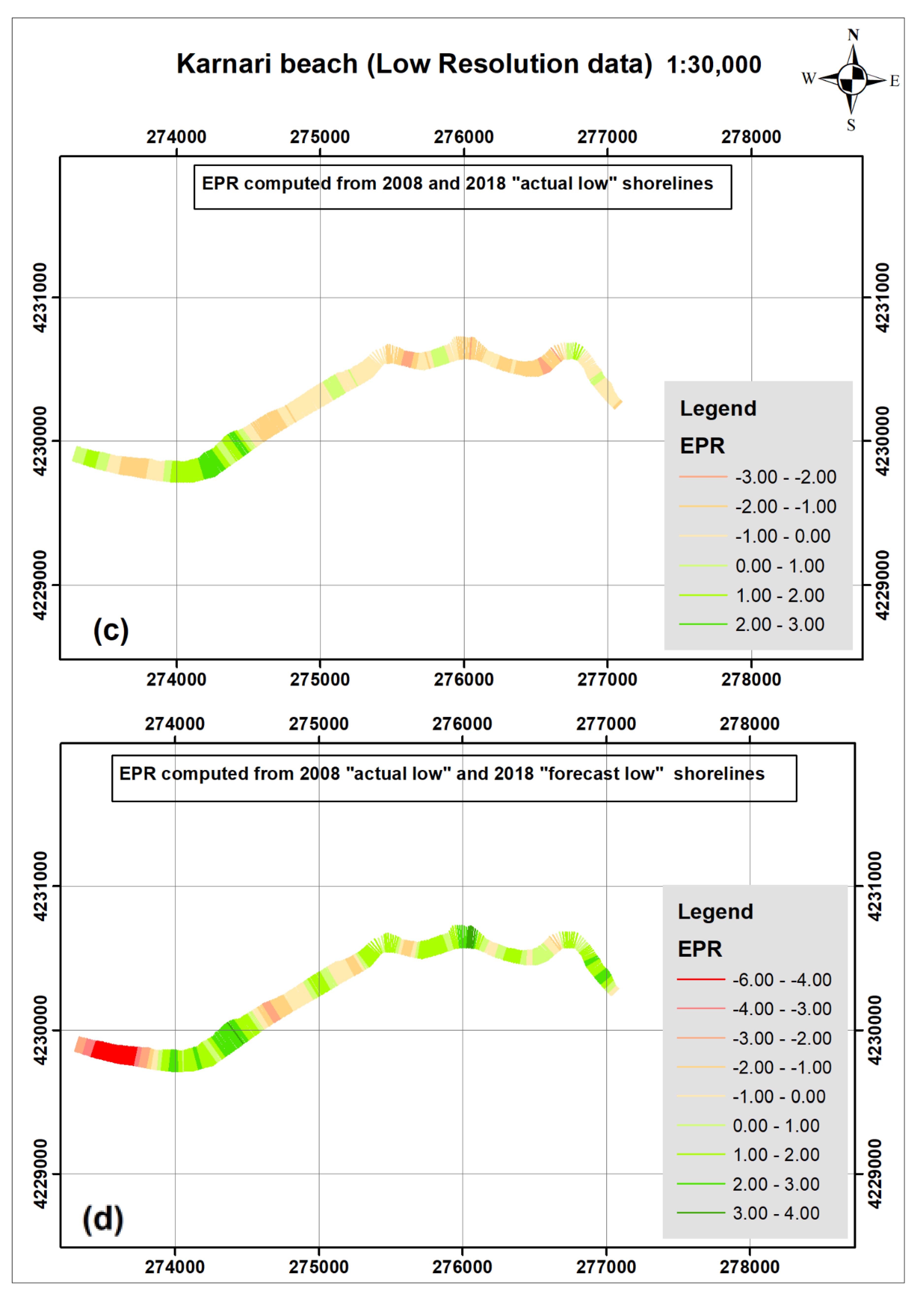
| Karnari Beach | |||||
|---|---|---|---|---|---|
| Data Resolution | Figures | Min | Max | Mean | Standard Deviation (σ) |
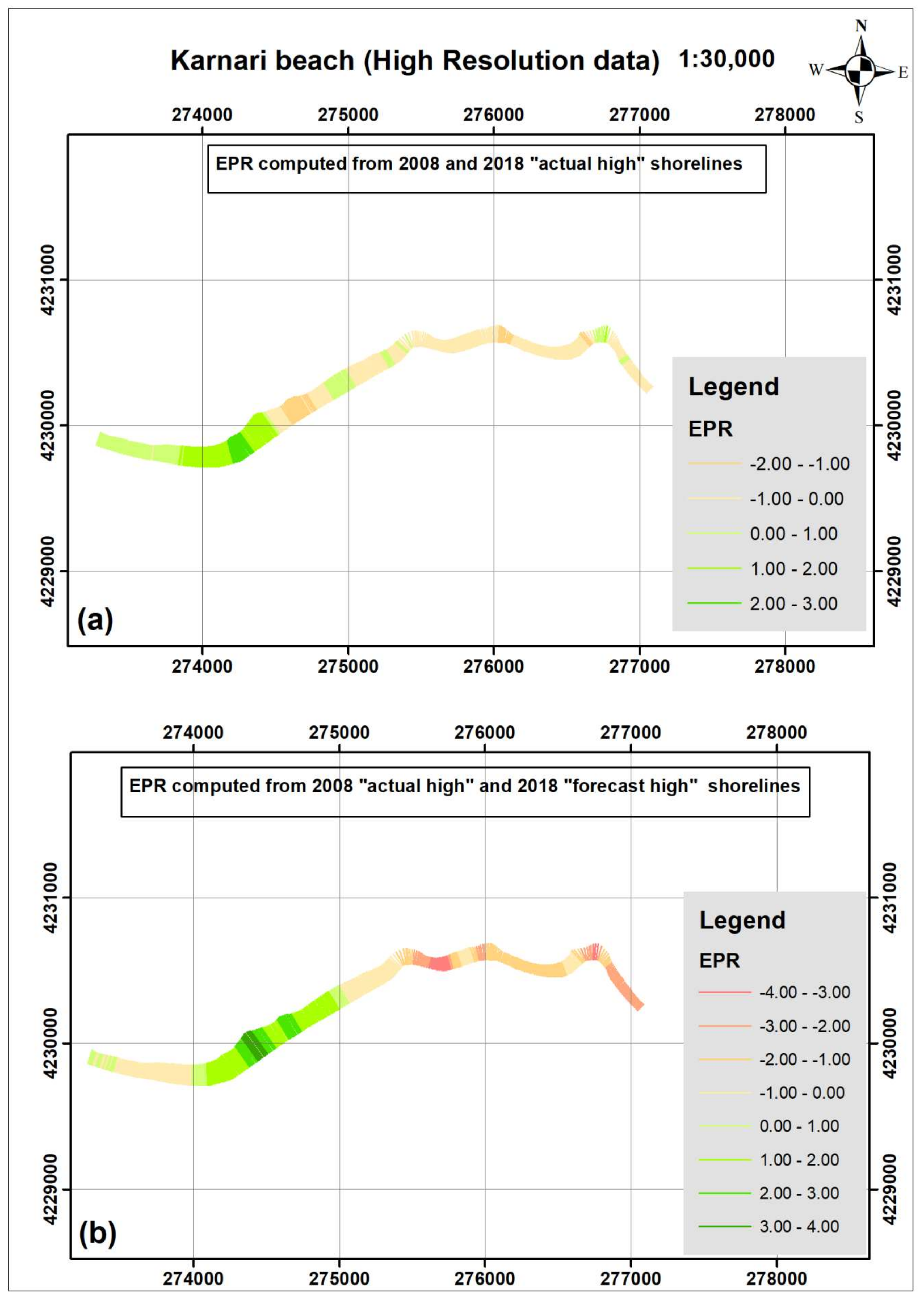
| 2008 and 2018 “actual high” | Figure 12 | −1.64 | 3.02 | 0.00 | 0.90 |
| 2008 “actual high” and 2018 “forecasted high” | Figure 12b | −3.94 | 3.74 | −0.43 | 1.65 |
| 2008 and 2018 “actual low” | Figure 12c | −3.06 | 2.86 | −0.28 | 1.18 |
| 2008 “actual low” and 2018 “forecasted low” | Figure 12d | −6.21 | 4.10 | 0.14 | 2.07 |
© 2020 by the authors. Licensee MDPI, Basel, Switzerland. This article is an open access article distributed under the terms and conditions of the Creative Commons Attribution (CC BY) license (http://creativecommons.org/licenses/by/4.0/).
Share and Cite
N. Apostolopoulos, D.; G. Nikolakopoulos, K. Assessment and Quantification of the Accuracy of Low- and High-Resolution Remote Sensing Data for Shoreline Monitoring. ISPRS Int. J. Geo-Inf. 2020, 9, 391. https://0-doi-org.brum.beds.ac.uk/10.3390/ijgi9060391
N. Apostolopoulos D, G. Nikolakopoulos K. Assessment and Quantification of the Accuracy of Low- and High-Resolution Remote Sensing Data for Shoreline Monitoring. ISPRS International Journal of Geo-Information. 2020; 9(6):391. https://0-doi-org.brum.beds.ac.uk/10.3390/ijgi9060391
Chicago/Turabian StyleN. Apostolopoulos, Dionysios, and Konstantinos G. Nikolakopoulos. 2020. "Assessment and Quantification of the Accuracy of Low- and High-Resolution Remote Sensing Data for Shoreline Monitoring" ISPRS International Journal of Geo-Information 9, no. 6: 391. https://0-doi-org.brum.beds.ac.uk/10.3390/ijgi9060391