Automated Geolocation in Urban Environments Using a Simple Camera-Equipped Unmanned Aerial Vehicle: A Rapid Mapping Surveying Alternative?

Abstract

GNSS positioning accuracy can be degraded in areas where the surrounding object geometry and morphology interacts with the GNSS signals. Specifically, urban environments pose challenges to precise GNSS positioning because of signal interference or interruptions. Also, non-GNSS surveying methods, including total stations and laser scanners, involve time consuming practices in the field and costly equipment. The present study proposes the use of an Unmanned Aerial Vehicle (UAV) for autonomous rapid mapping that resolves the problem of localization for the drone itself by acquiring location information of characteristic points on the ground in a local coordinate system using simultaneous localization and mapping (SLAM) and vision algorithms. A common UAV equipped with a camera and at least a single known point, are enough to produce a local map of the scene and to estimate the relative coordinates of pre-defined ground points along with an additional arbitrary point cloud. The resulting point cloud is readily measurable for extracting and interpreting geometric information from the area of interest. Under two novel optimization procedures performing line and plane alignment of the UAV-camera-measured point geometries, a set of experiments determines that the localization of a visual point in distances reaching 15 m from the origin, delivered a level of accuracy under 50 cm. Thus, a simple UAV with an optical sensor and a visual marker, prove quite promising and cost-effective for rapid mapping and point localization in an unknown environment.

1. Introduction

One of the most important factors for Global Navigation Satellite Systems (GNSS) in terms of desired positioning accuracy is ample satellite coverage. Nevertheless, GNSS sufficiency can be degraded in areas where the surrounding land morphology and geometry occludes or interacts with the signal between the satellites and the receiver. Specifically, urban environments and vegetated areas pose challenges to precise GNSS positioning because of signal interference, multipath effect or line of sight occlusion, factors which do not necessarily decrease over time during the measurement [1]. Typically, even a satellite signal blockage of short duration can significantly degrade performance in navigation systems. On the other hand, non-GNSS surveying alternatives, including total stations and laser scanners, involve time consuming practices in the field and/or costly equipment. There are cases where typical surveying cannot be substituted at the moment from GNSS, while in other cases classic surveying remains impractical. In between, there is an unresolved set of circumstances, where the need of cost-effective rapid mapping in GPS-denied environments remains crucial.

There are two main types of proposed solutions to resolve GNSS signal degradation, namely the ones that intervene with the GNSS signal per se, and those that use visual or other external aid to establish a precise coordinate estimation. Even though the performance of multi-constellation GNSS positioning in urban environment is improved with respect to independent system analysis [2], alternative techniques have been proposed, including angle approximation [3], shadow matching [4], multipath estimations using 3D models [5] and statistical models [6,7].

Several other solutions to this problem result from methods which work on improving GNSS positioning performance by introducing information from other modalities. In [2], the authors use a dead reckoning sensor, which is a spatial sensor comprising of 3-axis gyros, 3-axis accelerometers, 3-axis magnetometers, temperature and barometric altimeter to extrapolate a trajectory when there is no GNSS signal. Similarly, Kim and Sukkarieh [8] integrate a simultaneous localization and mapping (SLAM) system to a GNSS/Inertial Navigation System (INS) fusion filter. INS calculates the position of a moving object by dead reckoning without external references. In [9,10], the authors use post and real-time processing of high-resolution aerial images utilizing statistical techniques in order to georeference mobile mapping data extracted from GNSS-denied areas, while Heng et al. [11], proposed a platform for autonomous vehicle which performs real-time 3d mapping without the need of GNSS using a 360-degree camera system, multi-view geometry and fully convolutional neural networks. In [12], the authors combine an aerial (UAV) and a ground (computing processing) platform to georeference aerial data extracted by online visual SLAM based on ORB-SLAM2 algorithm utilizing photogrammetry techniques. Zahran et al. [5], apply machine learning to UAV sensors for detecting dynamic repeating patterns in the input signals, in order to improve the navigational states that are being estimated. The authors of [13] use visual odometry and extended Kalman filters in order to improve on inertial measurement unit (IMU) measurements Xu et al. [14], developed an ORB-SLAM method for real-time locating systems in indoor GPS-denied environments in order to detect characteristic points achieving an accuracy which ranges from 0.39–0.18 m aided by a depth sensor to acquire the scale information of the scene. Urzua et al. [4] attempted a SLAM method for localization in a GNSS-denied environment and solved the problem of scale, inherent in monocular SLAM methods, with a barometer and altimeter while a landmark recognition is used in [15]. However, they are limited by the availability of visual landmarks that the algorithm can compare against at high altitudes. Tang et al. [3] claim SLAM performance in featureless environments is poor and opt for a method without SLAM while in [16], a visual-based SLAM system for navigation using a UAV, a monocular camera, an orientation sensor (AHRS) and a position sensor (GPS) is proposed. The system performs SLAM processing for navigation but it fuses GPS measurements during initialization period to estimate the metric scale of the scene.

In this study, we propose a methodology that enables the localization of arbitrary points in an area of interest using only a single camera mounted on a commercial or other unmanned aerial vehicle (UAV or drone). More specifically, taking advantage of a single optical sensor’s visual feedback, the study’s methodology is able to provide efficient estimations of point coordinates which can be used in rapid mapping applications. The main objective of the proposed methodology is to propose, asses and in future establish, a surveying alternative for occluded or GNSS signal-degraded areas providing a point coordinate accuracy of 50 cm or better. This accuracy is acceptable in many topographic studies and it is most often much better compared to low satellite coverage GNSS measurements. For example, after a natural disaster incident, rapid mapping is quite important to assess the infrastructure damages and visually establish the new condition of the area [17]. Other cases include, mapping of natural resources [18,19] and search and rescue applications [20,21]. Drone- related studies only provide video feeds or images [22] sometimes with a rough estimation of positioning. Simple off the shelve UAV systems that use regular GNSS receivers, achieve accuracies in the 5 m range. When e.g., used in search and rescue applications this does not suffice, since precise geolocation of people in need is required, instead of broad positioning of the monitoring vessel. INS/IMU of corresponding simple commercial UAVs, again suffer from navigational errors accumulating by flying time. To the best of our knowledge and being quite active in the surveying field of work, there is no other established technique that covers these types of mapping in terms of accuracy, ease of use, cost and speed. Classic total station surveying is costly and slow, GNSS in occluded areas does not provide acceptable accuracy, classical photogrammetry is slow mainly in establishing the control points and in processing, more modern photogrammetry techniques like “direct georeferencing” are not cost-effective in terms of equipment because an attached GNSS receiver is required to the aerial vehicle platform [23,24] while laser scanners are quite expensive.

This work has been motivated by the need for a real-time autonomous rapid mapping technique of an unknown area where GNSS positioning is not accurate, or even impossible to acquire. A novel technique is presented based on SLAM and image processing. Urban environments do not suffer from limitations such as lack of features, as most obstructions of GNSS signals are objects that produce feature-rich visual representations that make the use of a SLAM method effective. No similar method exists that combines visual SLAM with transference of GNSS coordinates from one location to another based only on single basic camera sensors. The underlying incentive of this methodology is the optimization for simplicity, favoring less costly solutions in terms of equipment, in order to remain practical in a variety of settings. The proposed methodology does not depend on a GNSS receiver either, as it is assumed that the GNSS position of a visually identifiable location in the form of a manually placed marker, is available. Consequently, solving the problem by depending on correcting post processing procedures or using a variety of additional sensors (like a range finder or stereo camera) is avoided. The expenses for incorporating such sensors could lead to less flying time or implementation complexity for the UAV. Instead, the study’s use case enables to opt for a solution that includes only a UAV, a camera and a marker, with the possibility for either on-board or offline processing specifically tailored to the needs of the particular application. The remarkable point of this study is the ability to achieve accurate 3D localization of visual markers and rapid mapping in the order of 50 cm using just an off-the-shelve drone and a reference visual marker. This exact setting provides speed, efficiency, accuracy and low cost, that may constitute a revolution on modern surveying.

In the next section the main architecture, proposed methodology and implementation are presented. Next, two variations on the solution of the measurement methodology are compared, coupled with several experiments in Section 3, demonstrating the great potential of the method.

2. Materials and Methods

A significant milestone towards our goal is the identification of a marker pose in 3D space. These markers facilitate the identification of either known locations or locations of interest that need to be mapped. Estimations for the pose (which includes the location and rotation) of a marker can be extracted from images captured by a UAV-attached camera, identifying the pose of the camera at the time of image capture for multiple images along with pose information for the marker. By obtaining sufficient estimates for both poses, it is possible to combine the information required in order to accurately place the marker in the scene under a fixed or custom coordinate system. A class of methods that performs such a calculation are the SLAM methods which are able to map an unknown environment, localizing the sensor in the map in real time [25]. Hence, a monocular SLAM method is selected, through which it is possible to identify the pose of the UAV throughout the trajectory. In particular, the presented methodology is based on the OrbSlam2 [25] method, due to its performance compared to other monocular slam methods [26,27] which allows a UAV equipped with a camera to map its surroundings and localize itself in an unknown environment. The presented system is able to run online, while the UAV is in flight or off-board immediately after the flight while its initial output includes a point cloud estimation of the unknown environment and the extraction of camera pose information throughout the UAV flight. For the identification of arbitrary locations in the scene, visual markers are used, with the aid of ArUco library [6,28]. ArUco markers are synthetic square markers with a black border and an inner binary matrix that determines the marker’s identifier, meaning that different markers are given different identities. These markers define a custom coordinate system determining the coordinates of other elements in the scene, whether they are markers or points from the point cloud. Sensor-wise, the left optical sensor of a RealSense D435 camera (https://www.intelrealsense.com/depth-camera-d435/) was used, calibrated under factory-set parameters.

The presented methodology takes advantage of both the camera trajectory, in order to correctly estimate the markers/targets in a scene, as well as the point cloud, to provide visual cues about the form of the surrounding area and allow for measurements beyond the provided markers.

2.1. System Architecture

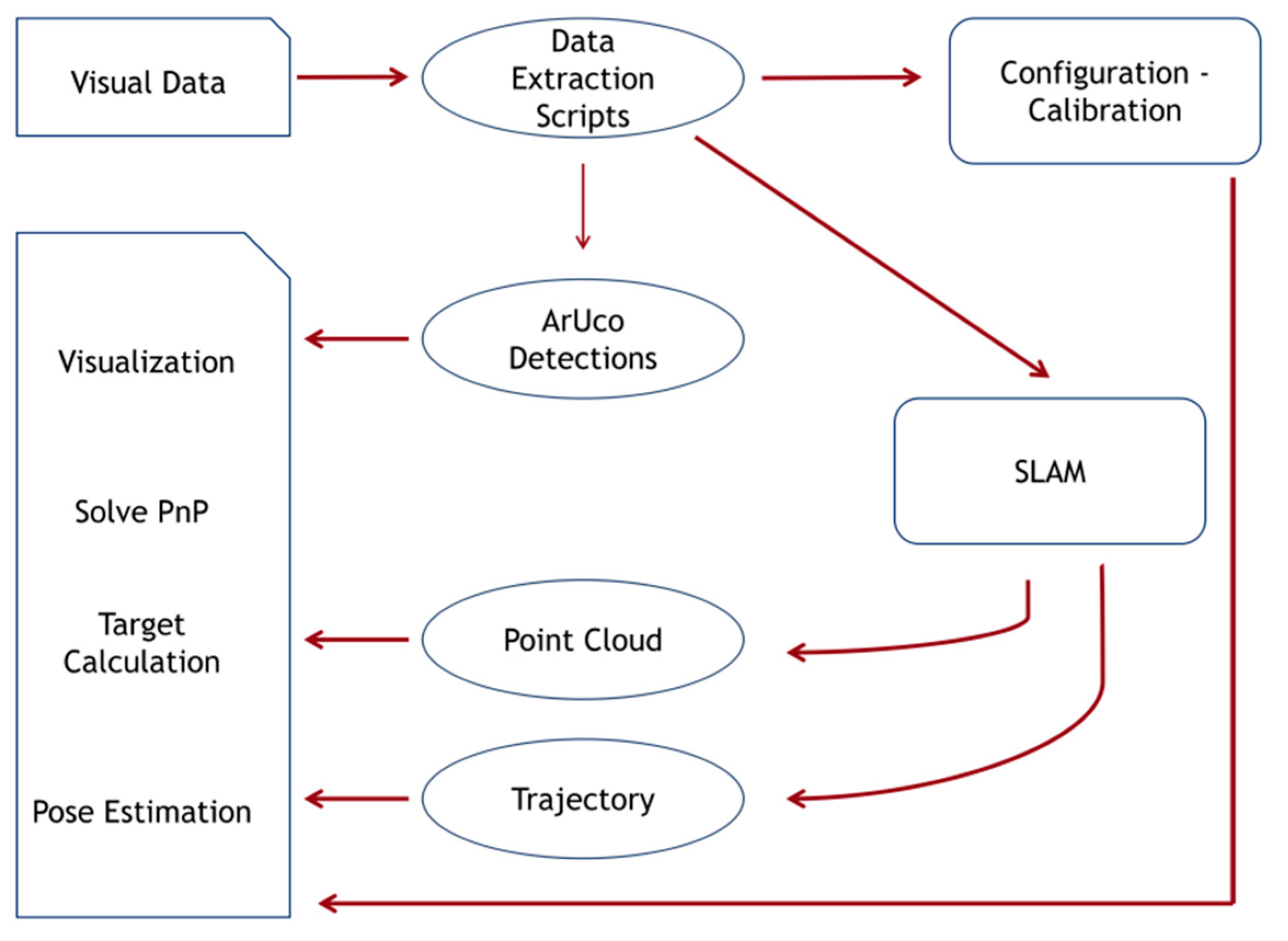
The overall methodology is outlined in the following schematic (Figure 1). To make the procedure as simple as possible, the origin marker may be placed right on the take-off drone platform.

The procedure consists of three stages. First, python scripts extract the data from inside a Robot Operating System (ROS, https://www.ros.org/) bag file which is captured by a single camera during the video recording process. The camera itself is used to obtain the calibration information from its factory settings while the image data stream is separated into frames and is stored in a folder. The following step is the SLAM processing of the image folder (Figure 2a), relating the image content with a camera trajectory and a point cloud.

The SLAM algorithm provides a mapping of the environment and allows the re-use of previously visited parts of an area through loop-closure, reducing the drift in the pose estimates of the camera after such a loop is detected. Loop-closure, or the re-visiting of previous parts of the trajectory is permitted while using a UAV to map an area, because its movement is not constrained to follow a pre-determined path to the target areas of interest.

Finally, the visual markers that aid the localization and detection of specific areas in the scene are detected in the images, and along with the point cloud and camera trajectory files, are given to a visualization algorithm. This algorithm produces a visual scene that includes the point cloud, the camera trajectory as well as the estimations of the visual marker locations in 3d space (Figure 2b).

2.2. Coordinate System Definition

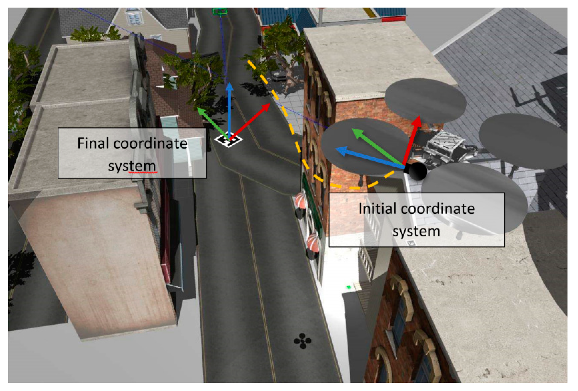
The initial coordinate system of the presented methodology is arbitrarily defined by ORB-SLAM2. This coordinate system is formed by the first camera frame in the captured video, where the x and y axes correspond to the right and top directions within the camera frame while the z axis points from the camera towards the scene. The ORB-SLAM2 algorithm initializes this coordinate system to align to the first recorded frame of the camera, with the positive direction of the x, y and z axis as described above. In this initial coordinate system an identity matrix as the rotation matrix, and a zero vector as the translation vector are defined in order for the initial coordinate system not to be affected by the following transformations.

Calibration data from the camera along with a camera pose obtained from the ORB-SLAM2 produced trajectory file are combined and used with OpenCV marker detection algorithms. The algorithm uses the camera calibration data and the camera pose, along with the 3d coordinates of a square that corresponds to the marker, and produces the rotation and translation vectors that transform points from the model coordinate system to the camera coordinate system. The camera pose of a frame is expressed inside the ORB-SLAM2 output trajectory file in relation to the original frame.

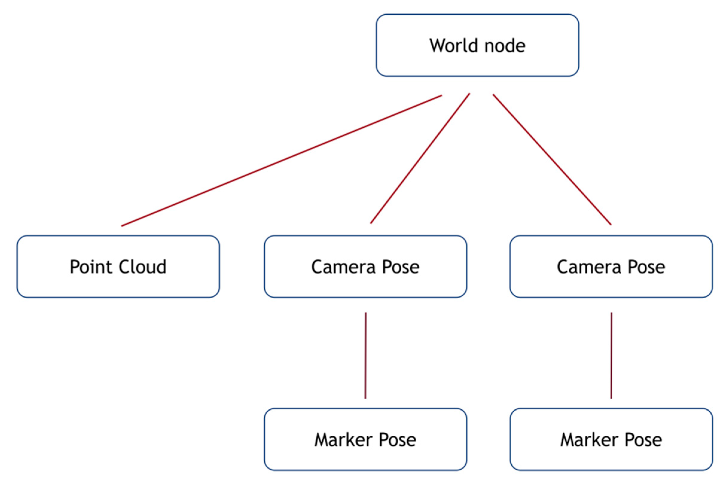
The presented implementation includes the construction of a scene graph, a tree structure of object nodes (Figure 3). The initial world node is the root of the tree structure which is connected with all other nodes with an identity rotation matrix and the zero-translation vector in order to remain fixed.

Given the translation and rotation (in Euler angles) of a node, its world position and world rotation are calculated. Each node that corresponds to a marker is assigned the vectors t, r and s to denote its translation, rotation and scale respectively. The vectors are local poses, in the coordinate system of the camera frame that detected the marker contained in the node:

$$\overrightarrow{\mathrm{t}}=\left[\begin{array}{c}\mathrm{x}\\ \mathrm{y}\\ \mathrm{z}\end{array}\right]\overrightarrow{\mathrm{r}}=\left[\begin{array}{c}\mathsf{\phi }\\ \mathsf{\vartheta }\\ \mathsf{\psi }\end{array}\right]\overrightarrow{\mathrm{s}}=\left[\begin{array}{c}{\mathrm{s}}_{\mathrm{x}}\\ {\mathrm{s}}_{\mathrm{y}}\\ {\mathrm{s}}_{\mathrm{z}}\end{array}\right],$$

(1)

where $\overrightarrow{\mathrm{t}}$, $\overrightarrow{\mathrm{r}}$, $\overrightarrow{\mathrm{s}}$ the translation, rotation and scale vectors stored inside a node.

To determine the world pose of a node, we define the S, T and R (2, 3) matrices in homogeneous coordinates:

$$\mathrm{S} =\left[\begin{array}{c}{\mathrm{s}}_{\mathrm{x}}\\ 0\\ 0\\ 0\end{array}\begin{array}{c}0\\ {\mathrm{s}}_{\mathrm{y}}\\ 0\\ 0\end{array}\begin{array}{c}0\\ 0\\ {\mathrm{s}}_{\mathrm{z}}\\ 0\end{array}\begin{array}{c}0\\ 0\\ 0\\ 1\end{array}\right], \mathrm{T} =\left[\begin{array}{c}\begin{array}{cc}1& 0\end{array} \begin{array}{cc}0& \mathrm{x}\end{array}\\ \begin{array}{cc}0& 1\end{array} \begin{array}{cc}0& \mathrm{y}\end{array}\\ \begin{array}{cc}0& 0\end{array} \begin{array}{cc}1& \mathrm{z}\end{array}\\ \begin{array}{cc}0& 0\end{array} \begin{array}{cc}0& 1\end{array}\end{array}\right],$$

(2)

$$\mathrm{R}=\left[\begin{array}{cccc}\cos \left(\mathrm{r}2\right)\cos \left(\mathrm{r}1\right)& \cos \left(\mathrm{r}2\right)\sin \left(\mathrm{r}1\right)\sin \left(\mathrm{r}0\right)-\cos \left(\mathrm{r}0\right)\sin \left(\mathrm{r}2\right)& \sin \left(\mathrm{r}2\right)\sin \left(\mathrm{r}0\right)+\cos \left(\mathrm{r}2\right)\cos \left(\mathrm{r}0\right)\sin \left(\mathrm{r}0\right)& 0\\ \cos \left(\mathrm{r}1\right)\sin \left(\mathrm{r}2\right)& \cos \left(\mathrm{r}2\right)\cos \left(\mathrm{r}0\right)+\sin \left(\mathrm{r}2\right)\sin \left(\mathrm{r}1\right)\sin \left(\mathrm{r}0\right)& \cos \left(\mathrm{r}0\right)\sin \left(\mathrm{r}2\right)\sin \left(\mathrm{r}1\right)-\cos \left(\mathrm{r}2\right)\sin \left(\mathrm{r}0\right)& 0\\ -\sin \left(\mathrm{r}1\right)& \cos \left(\mathrm{r}1\right)\sin \left(\mathrm{r}0\right)& \cos \left(\mathrm{r}1\right)\cos \left(\mathrm{r}0\right)& 0\\ 0& 0& 0& 1\end{array}\right]$$

(3)

where S, T, and R, represent scale, translation and rotation matrices. Multiplying these matrices results in the transformation matrix for the specific node. Since each node stores its local transform, the use of parent node transformation matrices in combination with the local transformation matrix can result in extracting the world coordinates for the node.

The world pose of any node that has a parent is determined recursively, by matrix multiplication between the G matrix of the parent and the T, R and S matrices (4). If a node has no parent, the matrix product of T, R and S are set to the identity matrix. After determining the world location of two nodes (the target marker node (6) and the origin node (7)), the translation vector between a target node and an origin node can be formed (5).

Recursively computing the local transformation matrices, and multiplying them together until reaching the world node, we are able to form the transformation G that gives the global transformation from the origin to the node’s pose and scale:

$$\mathrm{G} ={ \mathrm{G}}_{\mathrm{parent}} \mathrm{T}\cdot \mathrm{R} \cdot \mathrm{S},$$

(4)

$${\mathrm{t}}_{\mathrm{f}}={ \mathrm{R}}_{\mathrm{origin}} \cdot \left({\mathrm{t}}_{\mathrm{target}}-{\mathrm{t}}_{\mathrm{origin}}\right),$$

(5)

$${\mathrm{t}}_{\mathrm{target}}=\left[\begin{array}{c}{\mathrm{t}}_{\mathrm{x}}\\ {\mathrm{t}}_{\mathrm{y}}\\ {\mathrm{t}}_{\mathrm{z}}\\ 1\end{array}\right]$$

(6)

$${\mathrm{t}}_{\mathrm{origin}}=\left[\begin{array}{c}{\mathrm{o}}_{\mathrm{x}}\\ {\mathrm{o}}_{\mathrm{y}}\\ {\mathrm{o}}_{\mathrm{z}}\\ 1\end{array}\right]$$

(7)

The world node that is placed at the origin is coincidental with the coordinate system of the first key-frame produced by the ORB-SLAM2 system. Each camera node is attached to this world node. Therefore, the point cloud and camera poses are placed in the same coordinate system, as their values are initially defined in reference to that coordinate system in ORB-SLAM2. ArUco markers are attached to the camera node which detected them originally, and by combining the results of solvePnP (that places the relative ArUco marker pose in the camera coordinate system), with that of the camera pose, we can thereafter calculate the world position and rotation of each marker in the world coordinate system.

For every marker which is detected throughout the video capture a pose is estimated. It is the case that multiple detections lead to the same amount of marker poses. To obtain a final pose estimate for a marker, we average the locations of the set of filtered markers, and interpolate the quaternions to obtain a single pose estimate for each marker in the scene. At the same time, we only keep a percentage of the markers, based on where they lie if ordered by the amount of distance from the average location. We ignore secondary occurrences of markers in the video, as the earliest pose estimations are typically the most robust. The threshold for re-occurrence of a marker is set to two real-time seconds of absence from the frame (corresponding to 180 frames of zero detections of the specific marker at 90 fps).

The presented implementation is able to define the final coordinate system of the scene, represented by a single marker (the origin marker). It’s worth to mention that this is absolutely different from the initial ORB-SLAM2 coordinate system and should not be confused (Figure 4). The method of coordinate system definition, estimates the rotation matrix and translation vector from the pose of the origin marker, and places a coordinate system to the center of the marker which represents its origin. This pose is expressed from the world pose of the marker as estimated in relation to the original coordinate system of the ORB-SLAM2 initial frame. After the coordinate system definition, the implementation for calculating the final pose estimation of all markers is performed utilizing the final coordinate system defined by the origin marker.

2.3. Initial Approaches for Scale Estimation

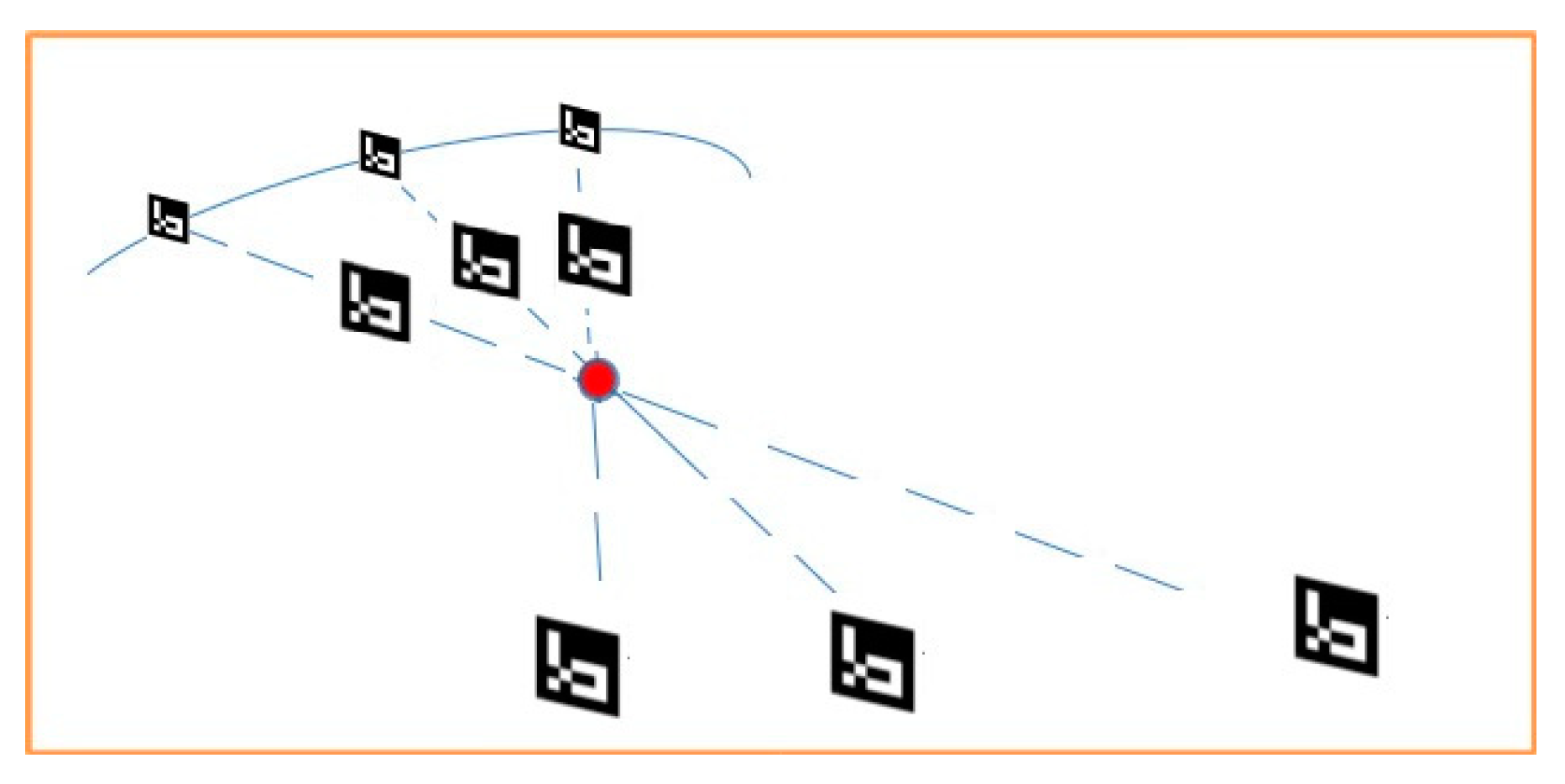
During the pose-estimation of a marker, its scale is not determinable from a single image in this monocular setup. An ArUco marker will have the same projection on the image whether it has a large size and is localized at a great distance from the camera or, inversely, when it is small and close to the camera. All the in-between locations of the marker form possible location-scale pairs in a line. Thus, the entire collection of images that contain a particular ArUco marker are taken into account. In order to estimate the local scale, the distances between all ArUco marker locations in the image collection need to be minimized. Several comparison methods were attempted without any significant differences, so the average of all pairwise distances between the markers was utilized as the comparison metric. By evaluating different scales for the ArUco markers, it was observed that this minimization converges when the markers approach their true size. Thus, initially this scale estimate was used to impose a scale on the entire model (trajectory and point cloud included). An illustrative example of this process is shown in the following Figure 5.

Multiple different possible scale estimates, one for each marker were obtained. The actual estimation of the 3d pose of the ArUco markers combines information from the camera coordinate system projections being transformed to world space. We use the camera-pose information to convert from the camera coordinates to the real-world coordinates. The SLAM monocular setup method is scale-agnostic but is able to confine the unknown scaling variable to a single value, instead of being per-axis, which simplifies the problem of scale estimation.

An alternative approach of scale estimation problem was performed with the assumption that two markers are accurately identified a-priori. The previous method was still used for estimating the correct marker scale, and average the marker positions to obtain the estimate of the position of a particular marker. Then, based on the absolute scale conversion factor between the two coordinate systems as the ratio of the distances between two markers, the first and second markers were chosen which are typically more accurate, being earlier in the trajectory path. The scale conversion factor was then used to convert from the Orb-Slam2 coordinate system units to the real world units. The actual location of any point in the Orb-Slam2 coordinate system is reprojected by taking the product of the location for each axis with the scale factor.

Although at first, the above initial approach seemed quite promising, it presented some issues in line with the accuracy of estimations and the efficiency of processing algorithms, a fact that leaded our research in a more sophisticated approach: The multiple line convergence method.

2.4. Multiple Line Convergence Method

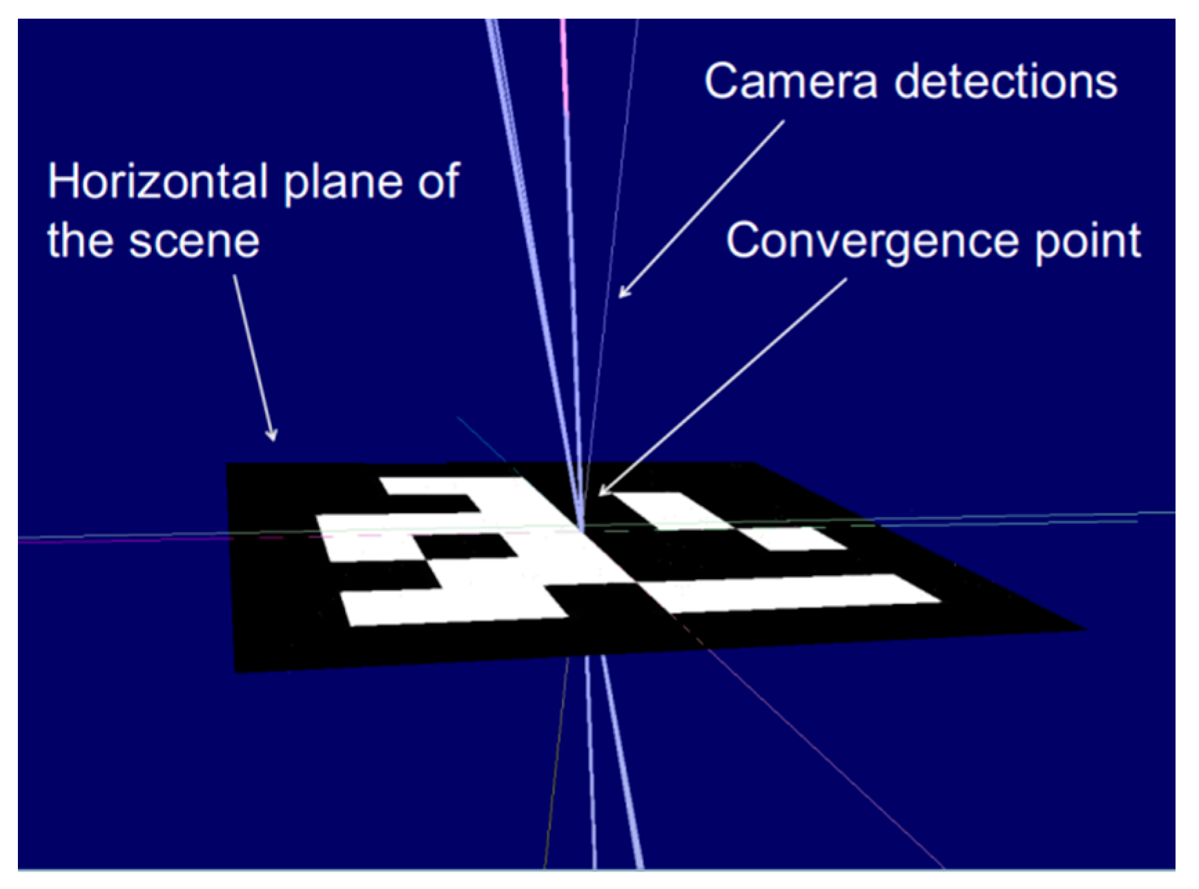
During experimentation, the pose estimates of the markers in 3d space, come from a routine that takes in the position of the corners of an ArUco marker, along with the marker size in the real world, the camera coefficients and the distortion parameters. When there are multiple marker detections, the method so far averages the locations of the markers and produces a single pose. These estimates can bias the estimate of the location of the marker, with a lot of poses being out of alignment with the point cloud.

The proposed implemented multiple line convergence method (MLCM), encounters this issue with a new approach. Instead of estimating each pose separately and combining them by averaging the translations and rotations (through quaternion interpolation), MLCM focuses on the line segments which connect each pose estimate with the position of the camera that detected the corresponding marker. This approach, leads to a new method of determining location: Even though the markers have locations that are above the designated ground truth, by changing the size of each marker, it is possible to align it with the ground truth coordinate in a much more precise fashion. However, the minor size changes are separate for each marker. At the same time, the lines that connect the center of each marker with the corresponding camera pose, if extended, all meet in the same area which corresponds to a location that aligns with the point cloud’s assumed surface (Figure 6).

This is reasonable, as the extension of the line provides all possible positions of the marker, given its corner position on the screen, for all possible marker sizes. Through experiments, it is determined that the location of the marker as a function of its size, corresponds with the line that is the extension of the line segment between the marker position and the camera pose, for any size.

The marker size that solvePnP uses to its real world size is set in meters. Then, pseudo-inverse least squares [29,30] optimization is used to obtain the point where all the connecting lines converge. The final equation is of the form S * p = C (13), where p is the least squares solution:

$${\mathrm{d}}_{\mathrm{i}}^2={\left[||\mathrm{p} -{ \mathrm{a}}_{\mathrm{i}}||\right]}^2-{\left[{\left(\mathrm{p} -{ \mathrm{a}}_{\mathrm{i}}\right)}^{\mathrm{T}}{ \mathrm{n}}_{\mathrm{i}}\right]}^2={\left(\mathrm{p} -{ \mathrm{a}}_{\mathrm{i}}\right)}^{\mathrm{T}}\left(\mathrm{p} -{ \mathrm{a}}_{\mathrm{i}}\right)-{\left[{\left(\mathrm{p} -{ \mathrm{a}}_{\mathrm{i}}\right)}^{\mathrm{T}}{ \mathrm{n}}_{\mathrm{i}}\right]}^2,$$

(8)

$${{\displaystyle \sum }}_{\mathrm{i}}{\mathrm{d}}_{\mathrm{i}}^2={{\displaystyle \sum }}_{\mathrm{i}}\left[{\left(\mathrm{p} -{ \mathrm{a}}_{\mathrm{i}}\right)}^{\mathrm{T}}\left(\mathrm{p} -{ \mathrm{a}}_{\mathrm{i}}\right)-{\left[{\left(\mathrm{p} -{ \mathrm{a}}_{\mathrm{i}}\right)}^{\mathrm{T}}{\mathrm{n}}_{\mathrm{i}}\right]}^2\right],$$

(9)

$${{\displaystyle \sum }}_{\mathrm{i}}\left[2\left(\mathrm{p} -{ \mathrm{a}}_{\mathrm{i}}\right)-2\left[{\left(\mathrm{p} -{ \mathrm{a}}_{\mathrm{i}}\right)}^{\mathrm{T}}{\mathrm{n}}_{\mathrm{i}}\right]{\mathrm{n}}_{\mathrm{i}}\right]=0,$$

(10)

$${{\displaystyle \sum }}_{\mathrm{i}}\left(\mathrm{p} -{ \mathrm{a}}_{\mathrm{i}}\right)={{\displaystyle \sum }}_{\mathrm{i}}\left[{\mathrm{n}}_{\mathrm{i}}{\mathrm{n}}_{\mathrm{i}}^{\mathrm{T}}\right]\left(\mathrm{p} -{ \mathrm{a}}_{\mathrm{i}}\right),$$

(11)

$$\left[{{\displaystyle \sum }}_{\mathrm{i}}\left[{\mathrm{n}}_{\mathrm{i}}{\mathrm{n}}_{\mathrm{i}}^{\mathrm{T}}- \mathrm{I}\right]\right]\mathrm{p} ={{\displaystyle \sum }}_{\mathrm{i}}\left[{\mathrm{n}}_{\mathrm{i}}{\mathrm{n}}_{\mathrm{i}}^{\mathrm{T}}- \mathrm{I}\right]{\mathrm{a}}_{\mathrm{i}},$$

(12)

$$\mathrm{S} \cdot \mathrm{p} = \mathrm{C},$$

(13)

Every line “i” is defined by the starting point “ai “ and its direction “ni” which is a unit vector. The distance between the center of each marker and the corresponding camera pose is defined by “di” while ${\left(\mathrm{p} -{ \mathrm{a}}_{\mathrm{i}}\right)}^{\mathrm{T}}{ \mathrm{n}}_{\mathrm{i}}$ is the projection of $\mathrm{p} -{ \mathrm{a}}_{\mathrm{i}}$ on the line “i”. In Equation (9), the sum of the distance squares “di” is minimized while in Equation (10), the derivative with respect to p is calculated with the aid of Equations (11) and (12) to form Equation (13).

The last line of the result is of the form S × p = C (13), where S is a 3 × 3 matrix, while C and p are 3 × 1 vectors. If p was the intersection point of all the lines, then S would be invertible, and multiplying by the inverse of S from the left would give us a closed form solution for p. However, due to errors in the estimate of the lines, they do not generally intersect at a single point. Consequently, least-squares optimization is used to minimize the distance of the point from all lines, by using the pseudo-inverse matrix S+ producing:

$$\mathrm{p} ={ \mathrm{S}}^{+} \cdot \mathrm{C},$$

(14)

Solving this Equation (14), and setting the world translation of each ArUco marker to the corresponding solution point p, we have a robust method for estimating the location of the markers.

2.5. Plane Alignment Method

An issue with marker pose estimation was that the origin marker’s pose defines the origin of a coordinate system. Extending the axes of that coordinate system, we compound any rotation errors in the marker pose estimation, so that estimating the pose of any other marker in the scene will produce translation errors because of axis misalignment. The placement of the ArUco marker is performed on a flat surface that determines the ground truth horizontal plane of the scene (Figure 6). Parts of this horizontal plane are estimated (with error) and assigned to points in the point cloud output of the SLAM algorithm.

In order to align the marker with the point cloud, plane segmentation is performed on the point cloud using the pcl python library. The segmentation process uses RANSAC algorithm to produce part of the point cloud that matches a plane while it gives access to the plane coefficients, in the form of ax + by + cz + d = 0.

At the same time, it is able to obtain the normal vector from the plane coefficients, forming n = [a, b, c]. The marker pose normal vector is determined by rotating the normal vector of a marker without rotation, so as to match the marker’s rotated pose, using the rotation matrix that each marker is associated with.

In the end, two normal vectors have been produced that will be matched if there is no need for alignment. In general, the marker pose will be slightly different from the desired pose. The normal vectors are not enough to define the entire pose of the marker, so the most appropriate way to align the marker with the point cloud is to perform a rotation that when applied on the pose normal vector, it aligns it with the plane normal vector. By expressing this rotation based on the normal vectors, it is able to apply it as a rotation matrix to the pose rotation matrix (through matrix multiplication), and define all three rotation angles at the same time:

$$\mathrm{G} =\left(\begin{array}{c}\mathrm{A}\cdot \mathrm{B}\\ ||\mathrm{A}\times \mathrm{B}||\\ 0\end{array}\begin{array}{c}-|| \mathrm{A}\times \mathrm{B}||\\ \mathrm{A}\cdot \mathrm{B}\\ 0\end{array}\begin{array}{c}0\\ 0\\ 1\end{array}\right)$$

(15)

$$\mathrm{u} =\frac{\left(\mathrm{A}\cdot \mathrm{B}\right)\mathrm{A}}{||\left(\mathrm{A}\cdot \mathrm{B}\right)\mathrm{A}||}= \mathrm{A}$$

(16)

$$\mathsf{\upsilon } =\frac{\mathrm{B} -\left(\mathrm{A}\cdot \mathrm{B}\right)\mathrm{A}}{||\mathrm{B} -\left(\mathrm{A}\cdot \mathrm{B}\right)\mathrm{A} ||}$$

(17)

$$\mathsf{\omega } = \mathrm{B}\times \mathrm{A}$$

(18)

$$\mathrm{F} ={\left(\mathrm{u} \mathsf{\upsilon } \mathsf{\omega }\right)}^{-1}={\left(\mathrm{A} \frac{\mathrm{B} -\left(\mathrm{A}\cdot \mathrm{B}\right)\mathrm{A}}{||\mathrm{B} -\left(\mathrm{A}\cdot \mathrm{B}\right)\mathrm{A} ||} \mathrm{B}\times \mathrm{A}\right)}^{-1}$$

(19)

$$\mathrm{U} ={ \mathrm{F}}^{-1}\cdot \mathrm{G} \cdot \mathrm{F},$$

(20)

Using the above formulas, a transformation matrix U is obtained (Equation (20)). The multiplication of U with a vector v expresses the rotation from A to B where A and B are the normal vectors of the solution. Instead of multiplying U with a vector, it can be multiplied with the rotation matrix corresponding to the pose of the marker to form a new pose. Then the normal of the marker will align with the plane normal.

The matrix U, when multiplied with the marker’s rotation matrix (U × R) forms a new rotation matrix that is aligned to the plane normal. In order for the algorithm to match enough points to obtain an accurate normal, a procedure of plane segmentation is performed on the entire point cloud while then, the procedure is applied again, but only locally (1 meter radius). Finally, the minimum distance between the most significant 1-meter radius plane normal and the set of normals from the entire point cloud is estimated. Thus, the plane normal is extracted from the entire point cloud, that matches the local plane normal best. By performing this procedure, it is possible to correct both the pose and rotation of an ArUco marker, leading to robust measurements, and a fine-tuned definition of the origin coordinate system, which is paramount to obtaining the final estimates for all ArUco markers that do not participate in defining the coordinate system.

3. Results

To validate the proposed methodology, an experimental setting was formulated, which was replicated eighty (80) times in order to define the optimal conditions which succeed the highest accuracy. Through the course of this study, three additional experimental indoor and outdoor sets have been conducted to assist development and optimization of the implemented methodology. All provided comparable results to the final set presented herein.

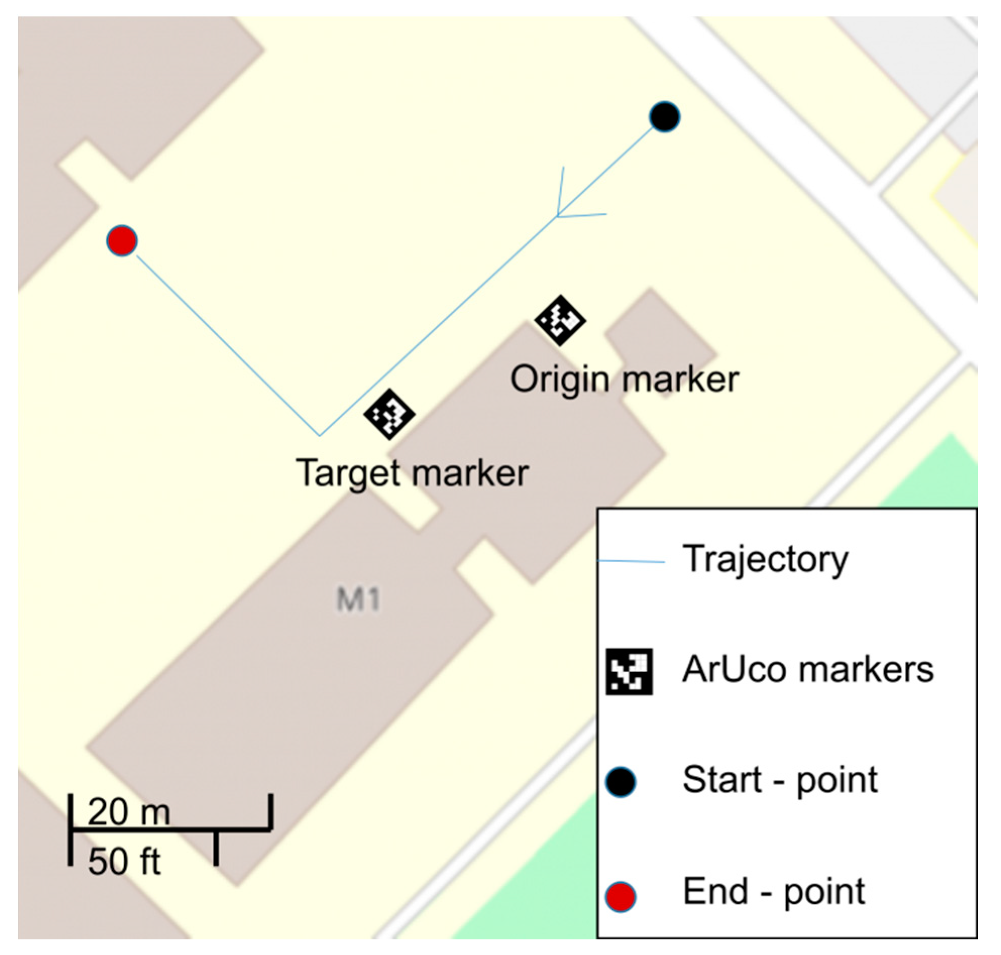
For the implementation of the experiment, two ArUco markers with a size of 0.20 m each were used and placed near a building to define the origin and the target respectively. The origin marker is typically used as a reference point for the target marker in the scene, since its pose is assumed to be known. Specifically, the origin marker is defined with the coordinates 0, 0, 0 in X, Y and Z axes, while the ground truth relative coordinates of the target marker are measured using the reference point (origin marker). The optical sensor of the camera has a resolution of 1280 × 800 pixels, sensor aspect ratio 8:5, focal length 1.93 mm, fixed focus, while the image format is 10-bit RAW.

The camera follows a trajectory that approaches a right-angle shape; the target marker is to be detected at the end of the trajectory, while the origin marker is detected soon after the beginning of the video capture. In all replicates of the experiment the videos are recorded at 90fps using 848 × 480 resolution. The area under mapping is an urban area including buildings and man-made objects, cars, along with vegetated regions. (Figure 7). Initial and validation measurements of the area were performed through total stations, electronic distance measurers and GNSS receivers.

The conditions and techniques that impact the results and are taken into account in each set of experiments are the following:

• Camera orientation through capturing the scene;
• Camera pace speed;
• Illumination conditions of the scene;

Concerning the camera orientation, it has been observed that the proposed methodology extracts more accurate results when the camera looks at the horizon instead of the floor because in the monocular setup there is no depth information like in a stereo mode setup and the algorithms need more information about the surroundings (e.g., buildings, cars, trees) in order to perform more accurate estimations of the mapping area. However, it is crucial for the camera to target the markers when it is close to them for their pose estimation. The ideal camera speed is about 3.5–4.0 km/h because the extracted video contains adequate amount of data for efficient processing. In higher speeds the system is possible to lose important information due to tracking loss of the SLAM algorithm while in lower speeds the processing algorithms become time consuming without any improvement on the results. Another factor that impacts the results is the illumination. It is observed that the system encounters issues to detect the target marker under low lighting conditions, e.g., high shadowing due to heavy clouds.

Following the above procedure, a multiple set of experiments was performed with the same setup. The output of each experiment contains a point cloud that maps the area of interest, the trajectory of the camera, the relative coordinates estimation of the target marker and the estimation of the distance between the origin and the target marker.

The ground truth of the target marker relative coordinates are: X: 53.2 cm, Y: 1570 cm Z: 0 cm. Z coordinate is defined as zero because the marker was placed in a leveled, smooth ground without altitude differences. The following experimental results are gradually presented to include (a) a single typical measurement to acquire a first comprehension of the results and simple statistics, (b) and (c) a twofold clustered group of measurements that delivered “higher” and “lower” accuracies and (d) an overall, all-inclusive outcome. In

Table 1. Typical example of coordinates and distance estimations.

Target Marker	X	Y	Z	Distance
Ground Truth	53.2 cm	1570	0 cm	1570.9 cm
Estimations	73.3 cm	1582.5 cm	8.8 cm	1584.2 cm
Error	20.1 cm	12.5 cm	8.8 cm	13.3 cm

, an example of a typical experiment where ground truth, estimations and related error of the target marker are depicted:

The X, Y, Z and distance errors were calculated by the difference between the estimated coordinates and the corresponding measured ground truth.

Most of the experimental results demonstrated that the relative coordinates of the target marker and the distance between the origin and target markers had a horizontal error (RMSExy) of 26 cm (see

Table 2. “Superior” experimental cluster error results.

Target Marker	X Error	Y Error	Z Error	Distance Error
Average	19.0 cm	14.6 cm	4.1 cm	15.0 cm
Std. Deviation	5.9 cm	8.0 cm	3.0 cm	8.3 cm
RMSE	19.8 cm	16.3 cm	4.9 cm	16.9 cm
RMSE xy	25.6 cm		-	-

). After conducting the whole set of experiments, two distinct clusters of accuracies were revealed (Table 2 and

Table 3. Lower accuracy experimental cluster error results.

Target Marker	X Error	Y Error	Z Error	Distance Error
Average	26.0 cm	38.6 cm	6.4 cm	39.4 cm
Std. Deviation	14.0 cm	16.1 cm	4.3 cm	15.9 cm
RMSE	29.0	41.4 cm	7.5 cm	42.1 cm
RMSE xy	50.5 cm

). This fact, as discussed later, can prove quite beneficial in providing enhanced coordinate estimations, since measurement repetition may force towards a higher accuracy solution. In Table 2, the average x, y, z and distance errors, the standard deviation and the RMSE errors of the results that had a clustered distribution around 15cm are presented:

As presented in Table 2, the difference between the ground truth and estimation of target marker has an average and RMSE error of 19 cm with standard deviation of about 6 cm in X axis while in Y axis and distance, the average and RMSE errors are about 15 and 16 cm respectively with a standard deviation of 8 cm. The lower error is contained in Z axis which is about 4 cm with a standard deviation of 2.9 cm.

In some iterations of the experiment, the results had lower accuracy with a horizontal error (RMSE xy) of 50.5 cm; The average and the standard deviation of these results are presented in Table 3:

In the set of experiments that is taken into account in Table 3, the accuracy is decreased mainly in Y axis and in distance estimation. Specifically, in X axis the error has an average of 26 cm with a standard deviation of 14 cm and an RMSE error of 29 cm while there is a significant average and RMSE error in Y and in distance which is about 40 cm with a standard deviation of 16 cm. During experimentation it was observed that estimations in Y axis were more error-prone than estimations in X and Z axes because the origin and target marker were placed in greater distance on Y axis and as a result, accidental aberrations from the defined conditions during the experiment, were able to influence the Y and by extension the distance estimations. Concerning the Z axis, the high accuracy of estimations is maintained in those sets of experiments also, with an average and RMSE error of about 7.0 cm and a standard deviation of 4.5 cm.

In order to have an overall estimation of this study’s methodology accuracy, the average and standard deviation of differences between the ground truth and the estimations of target marker and the RMSE errors taking into account all the experiment iterations are provided (

Table 4. Overall experimental error results.

Target Marker	X Error	Y Error	Z Error	Distance Error
Average	22.8 cm	27.5 cm	5.3 cm	28.2 cm
Std. Deviation	11.2 cm	17.6 cm	3.8 cm	17.7 cm
RMSE	25.2 cm	32.3 cm	6.4 cm	32.9 cm
RMSE xy	41.0 cm

).

As presented in Table 4, X axis has an average of about 23 cm with a standard deviation of about 11 cm and an RMSE error of 25 cm while in Y axis and distance, the average is about 28 cm with a standard deviation of 18 cm and an RMSE error of 32 cm. Z axis has the highest accuracy with an average of about 5.5 cm, a standard deviation of about 4 cm and an RMSE error of 6.5 cm. Finally the horizontal error (RMSE xy) taking into account all the experiment iterations is about 41 cm.

4. Discussion

Through this study, a novel methodology for rapid mapping in GNSS-denied environments is proposed. The methodology localizes markers and arbitrary points in an unknown environment using a UAV equipped with a single camera. The UAV travels through a flight path and identifies one or two pre-determined markers that have been assigned a known location and estimates their location. At first, a local coordinate system is defined for the scene with origin defined by the initial marker with known location, while consequently, the relative coordinates of the target markers are calculated using the developed multiple line convergence and plane alignment methods. During experimentation, the main challenge was the localization of a target visual point in a distance of about 16 m from the origin. The proposed methodology achieved a horizontal error less than 50 cm and vertical error less than 10 cm which is quite remarkable considering the minimal equipment used.

The estimations of marker coordinates are significantly close to the coordinates of ground truth given that in the experimental sets, a single optical sensor was used. All iterations of the experiment were performed over a period of a month under similar conditions: The UAV followed a trajectory with a right-angle shape while the markers had a ground truth distance of about 16 meters. During the analysis of the results, it was observed that after eighty (80) repetitions the errors were distributed in two distinct clusters: The first cluster represents the majority of the results with a horizontal error (RMSE xy) below 30 cm while the second cluster represents some iterations of the experiment with lower accuracy in Y and Distance estimations (40 cm). Table 2 which presents the statistical parameters of the first cluster, demonstrates that the methodology is able to estimate a target marker with a horizontal accuracy of 25 cm and a vertical accuracy of 5 cm. Table 3 which presents the statistical parameters of the second cluster, indicating a reasonable accuracy in X axis and a high accuracy in Z axis while Y and distance estimations suffer from an increased error with an average of 40 cm and a standard deviation of about 16 cm. This error is justified, since in Y axis the markers have greater distance (about 16 m) which is influences the accuracy if accidental aberrations happen during the performance of the experiment which diverge from the defined conditions. Finally, Table 4 which presents the statistical parameters of all iterations of the experiment results, validating the methodology with an overall horizontal accuracy of 41 cm and a vertical accuracy of 6.5 cm.

This analysis aligns with this study’s main goal of obtaining 50 cm-level precision in the identification of arbitrary locations in the scene as long as they are not very far from a location that has been previously geo-referenced. The local coordinates of a single characteristic point are transferred to different positions in real time when reception of the GNSS signal is not adequate for localization. Furthermore, it is possible to provide coordinates in a global coordinate system.

But how can this methodology address a real-world mapping task? First, when rapid mapping is the objective of a study, this method provides a great potential mainly due to its simplicity in measurement and equipment requirements. Through a single drone using a regular camera, one may obtain thousands of point coordinates in a few minutes within an accuracy of 50 cm or less. But the underlying power of the proposed methodology at its current stage, is that the method estimates its accuracy without the need of an additional post processing validation procedure. Through the target markers or loop closure, at the end of the mapping procedure the user will know the overall accuracy of the method which may span from a few centimeters to 50 cm. Due to the quite large error variance and clustering of the accuracies in two main sets, which is related to the local conditions, the user may select to rerun the mapping procedure, if the accuracy estimation is at its upper bounds. Thus, if the results are unsatisfactory, there is a possibility by varying illumination conditions or camera pose, to obtain much better results. This information is available to the users at the end of the processing which can be completed in situ. In other words, the drone may pass twice over the area of interest collecting image/video feeds under varying conditions and camera orientation, in order to assist the algorithms to possibly provide optimized results.

5. Conclusions

This study, proposed a methodology that maps a GNSS signal-degraded area of interest, providing an acceptable accuracy for rapid mapping applications. The study’s methodology, combines a SLAM algorithm (ORB-SLAM2) with image processing, and computational geometry techniques in order to localize characteristic points in a local coordinate system with an accuracy of 50 cm or better. The main contribution of this study, is that provides a cost-effective approach in terms of equipment, since only a UAV, a single optical sensor, and a visual marker is required in order to perform localization of target points and mapping of the area of interest. Compared to other methodologies the UAV does not require a GNSS receiver, nor an IMU. The marker used can be deployed near the area of interest, close to the UAV’s take off site, providing a quick deployment compared to other techniques that require time consuming distribution of ground control points (GCPs).

Although the methodology introduces a surveying alternative procedure for rapid mapping projects, some aspects of the methodology could be improved. The final goal of this study is the autonomous attitude of the UAV and corresponding adjustments to provide optimal measurements towards rapid mapping of an unknown environment using only a UAV, a single optical sensor and at least one visual marker. The objective is that the optimization may reduce the overall level of accuracy to less than 30 cm, under varying conditions and settings. The error on the test site was estimated with the help of topographic–GNSS equipment. In the course of this study, at least three other sets of experiments on other test sites (indoors and outdoors) were conducted, demonstrating comparable results with the final test set, presented herein. In order to further test, optimize and standardize our method, extensive experimentation should take place in varying environments, while IMU and GNSS assisted statistical methods could be compared. Other means to compare and enhance the accuracy of rapid mapping which we already conduct acquiring less than 10 cm error, is by using different optical sensors such as a depth stereo camera. Yet, all these procedures stray away from our initial objective which is to push the accuracy levels of rapid mapping using common, off the shelve UAVs and a minimum cost printed marker.