Change Detection from Remote Sensing to Guide OpenStreetMap Labeling

Abstract

The growing amount of openly available, meter-scale geospatial vertical aerial imagery and the need of the OpenStreetMap (OSM) project for continuous updates bring the opportunity to use the former to help with the latter, e.g., by leveraging the latest remote sensing data in combination with state-of-the-art computer vision methods to assist the OSM community in labeling work. This article reports our progress to utilize artificial neural networks (ANN) for change detection of OSM data to update the map. Furthermore, we aim at identifying geospatial regions where mappers need to focus on completing the global OSM dataset. Our approach is technically backed by the big geospatial data platform Physical Analytics Integrated Repository and Services (PAIRS). We employ supervised training of deep ANNs from vertical aerial imagery to segment scenes based on OSM map tiles to evaluate the technique quantitatively and qualitatively.

Data Set License: ODbL

1. Introduction

It is natural to ask how the growing amount of freely available spatio-temporal information, such as aerial imagery from the National Agriculture Imagery Program (NAIP), can be leveraged to support and guide OpenStreetMap (OSM) mappers in their work. This paper aims at generating visual guidance for OSM [1] mappers to support their labeling efforts by programmatically identifying regions of interest where OSM is likely to require updating.

The outlined approach is based on translating remote sensing data, in particular vertical aerial images, into estimated OSMs for the regions contained in the image tiles. This first step exploits an image-to-image translation technique well studied in the deep learning domain. In a subsequent stage, the estimated OSM is compared to the current map to produce a “heat map”, highlighting artifacts and structures that alert mappers to locations that require updates in the current OSM. The output provides computer-accelerated assistance for the labeling work of OSM volunteers.

1.1. OpenStreetMap Data Generation Assisted by Artificial Neural Networks

OpenStreetMap is an open-data, community-driven effort to join volunteers in order to map the world. It provides a platform to label natural artifacts and human infrastructure such as buildings and roads manually. Labeling is largely a manual process done through an online tool that allows the submission of artifact definitions and their Global Positioning System (GPS) coordinates on top of geo-referenced satellite imagery [2].

It is difficult to maintain consistent global coverage with this manual process given the growth of data volume in OSM, as well as the number of artifacts and structures to be mapped. At the beginning of 2018, the compressed overall OSM Extensible Markup Language (XML) history file was 0.1 terabytes (TB) (2 TB uncompressed). Five years earlier, the historical data was less than half, about 40 gigabytes (GB) compressed. A back of the envelope calculation shows the effort involved in the creation and update of labels:

Assuming an OSM community member adds a new vector data record (nodes, ways, and tags in OSM parlance) of order of tens of kilobytes (KB) in minutes, the time invested-to-real time ratio reads:

$$\begin{array}{cc}\hfill =& \frac{\mathrm{estimated}\mathrm{time}\mathrm{invested}\mathrm{by}\mathrm{one}\mathrm{OSM}\mathrm{mapper}\mathrm{to}\mathrm{label}\mathrm{all}\mathrm{data}}{\mathrm{total}\mathrm{time}\mathrm{to}\mathrm{collect}\mathrm{all}\mathrm{OSM}\mathrm{data}}\hfill \\ \hfill =& \frac{\mathrm{compressed}\mathrm{OSM}\mathrm{data}\mathrm{size}·\mathrm{decompression}\mathrm{factor}/\left(\mathrm{mapper}\mathrm{label}\mathrm{speed}\mathrm{bit}\mathrm{rate}\right)}{\mathrm{total}\mathrm{time}\mathrm{to}\mathrm{collect}\mathrm{all}\mathrm{OSM}\mathrm{data}}\hfill \\ \hfill =& \frac{60·{10}^{6}KB·20/(20KB/60s)}{5·365·24·60·60s}\hfill \\ \hfill \sim & {10}^6/(4·{10}^4)\sim 25.\hfill \end{array}$$

(1)

Thus, approximately, an estimated 20 to about 30 mappers would need to work around the clock to generate OSM labels. This raises the question of whether the process can be automatized, generating a labeled map from geo-referenced imagery.

1.2. An Approach to OSM Generation Based on Deep Learning

One technique for producing maps from geo-referenced imagery is to treat the problem as a two step process in which pixel-wise segmentation is performed before pixels are grouped into vectorized entities like building outlines or road networks. Modern approaches to the segmentation problem typically use some form of encoder-decoder architecture incorporated into the ANN. These techniques employ an encoder to down-scale and a decoder upscale subsequently an image. Examples of such architectures are Mask R-CNN [3], SegNet [4,5], Pix2Pix [6,7], and U-Net [8]. See Appendix A for a primer on these architectures.

It becomes clear that segmentation may be formulated as a generic image-to-image mapping task. This approach is implemented and studied in this work. In particular, applying a numerical saddle-point optimization scheme This is also known as the minimax problem [9]. For details given the context of the CycleGAN training procedure, see Appendix A and [10].), the CycleGAN [11,12]—a system of cyclically-trained generative adversarial networks (GAN), to be precise—manages to establish a mapping between two sets of images, even without the need for any pixel-to-pixel correspondence of pairs of images from the sets. Among others, an intuitive description of the methodology is provided in Section 2.3.

1.3. Related Work

The challenge to identify human infrastructure from vertical aerial imagery has attracted an increasing amount of attention in recent years. Research in this field has advanced, e.g., on building detection [13,14,15], land use classification [16,17,18,19], and road network identification [20,21,22,23,24,25,26,27]. Among others, these approaches vary in the data used. While several of the previously cited publications directly estimate the outline of a road network from images, others use the GPS data or GPS trajectories. Returning to the general problem of map generation, References [28,29,30,31] are conceptually closest to our approach of image-to-image translation with the CycleGAN. A collection of literature references is maintained by the OSM community in a wiki consisting of various works of machine learning related to the OSM project [32].

1.4. Contributions

This paper reports our progress in applying deep learning techniques to generate OSM features. In particular, we focus on buildings and road infrastructure. Section 2.2 provides some detail on our management of geospatial images using the IBM PAIRS database. The remainder of Section 2 delves into the ANN design, training, and inference. The set of experiments described in Section 3 forms the basis of both intuition and quantitative analysis of the potential and hurdles to implementing a deep learning approach to OSM generation. Visual inspection of our data is used to explore aspects of image-to-image translation in the context of OSM data change detection from vertical aerial imagery in Section 4. As Supplemental Material, Appendix A provides a technical primer regarding deep learning in the context of our specific approach.

The contribution of this study is summarized as follows:

• We demonstrate the application of a modified CycleGAN with an attention mechanism trained on NAIP vertical aerial imagery and OSM raster tiles.
• We quantify the accuracy of house detection based on the approach above and compare it to a state-of-the-art house detection network architecture (U-Net) from the remote sensing literature.
• We exemplify the extraction of a heat map from the big geospatial data platform IBM PAIRS that stores OSM raster tiles and maps generated by the modified CycleGAN. This way, we successfully identify geospatial regions where OSM mappers should focus their labor force.
• We provide lessons learned where our approach needs further research. In the context of OSM map tiles that assign different colors to various hierarchies of roads, we inspect the color interpolation performed by the modified CycleGAN architecture.

2. Materials and Methods

Automated detection of human artifacts using ANNs requires structured storage and querying of high-resolution aerial imagery, cf. Section 2.2, as well as efficient handling of the intermediate outputs of the training process. Our work leverages the PAIRS remote sensing image repository for this task. The basics of image storage and retrieval in PAIRS covers Section 2.1. Sufficient discussion is provided, and the reader is encouraged to use the PAIRS engine via its public user interface [33] to explore the data used in this paper. Finally, Section 2.3 presents the design chosen for the ANN used to provide the results and insights of Section 3 and Section 4.

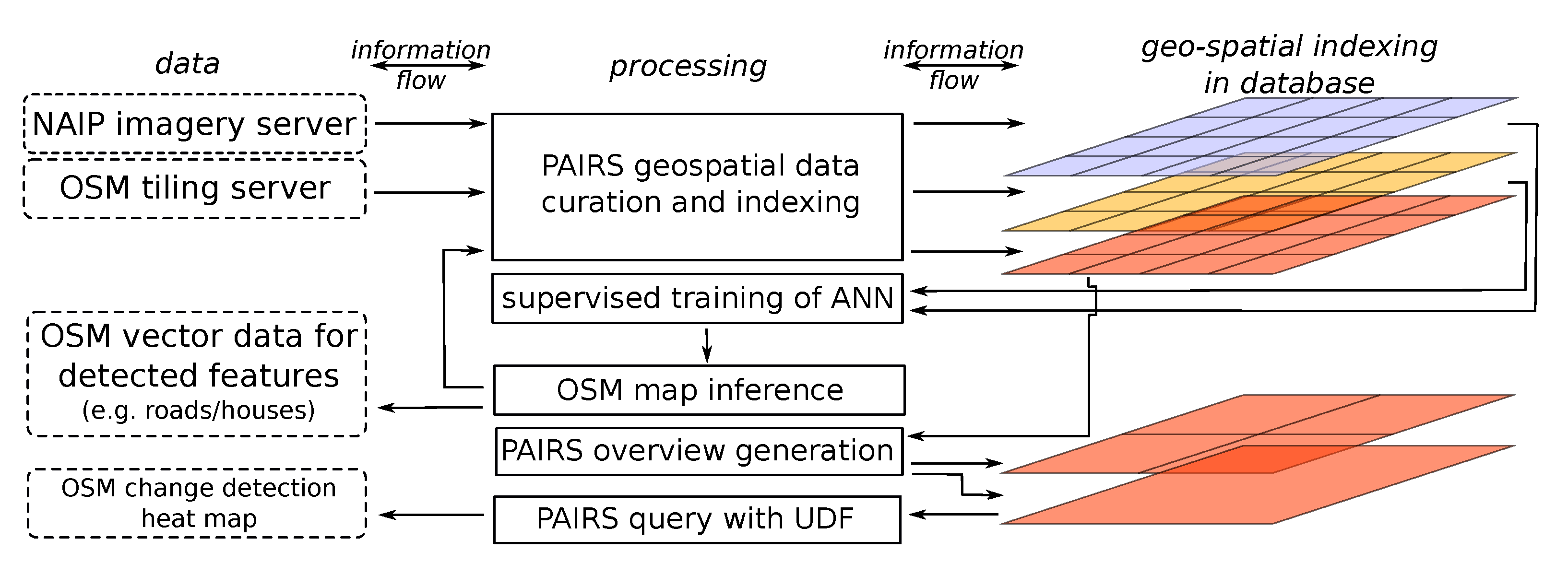
2.1. Scalable Geo-Data Platform, Data Curation, and Ingestion

The PAIRS repository [34,35,36] is intended to ingest, curate, store, and make searchable data by geo-temporal indexing for many types of analysis. PAIRS falls within the category of databases developed explicitly to optimize the organization of geo-spatial data [37,38,39]. Applications built on PAIRS range from remote sensing for archeology [40] and vegetation management [41] to the curation and indexing of astronomical data [42]. PAIRS maintains an online catalog of images for real-time retrieval using an architecture based on Apache HBase [43] as a backend store.

A major strength of the platform is the ability to scale, project, and reference images of differing pixel resolution onto a common spatial coordinate system. As noted above, imagery comes from many sources, resolution levels, and geospatial projections. A key function of the PAIRS data ingestion phase is to rescale and project raster images from all sources onto a common coordinate system based on the EPSG:4326/WGS 84 [44,45] Coordinate Reference System (CRS). The internal PAIRS coordinate system employs a set of nested, hierarchical grids to align images based on their resolution. This works as follows: PAIRS defines a resolution Level 29 to be a square pixel of exactly ${10}^{-6}$ Deg × ${10}^{-6}$ Deg in longitude and latitude. Resolution levels are increased or decreased by factors of two in longitude and latitude at each step such that the pixel area decreases or increases quadratically. Level 28 pixels are 2 $\times {10}^{-6}$ Deg × 2 $\times {10}^{-6}$ Deg, and so on. The PAIRS Level 26 approximately corresponds to a resolution of 1 × 1 meter at the Equator—this can also be conceived of as a QuadTree [46].

For example, during the ingestion of a raw satellite image tile to a specified level of 23, the ingestion pipeline performs the necessary image transformations to rescale the original pixels to a size of 64 $\times {10}^{-6}$ Deg × 64 $\times {10}^{-6}$ Deg. Rather than store individual pixels per each row of the database, the transformed image is partitioned into an array of 32 × 32 pixels called a “cell”. The cell is stored in HBase using a row key based on the longitude and latitude of the lower left corner of the cell at the resolution level of the cell. A timestamp of when the data was acquired is added to the key. A cell is the minimal addressable unit of image storage during queries.

This system of storing aligned and scaled images front loads the ingestion pipeline with CPU intensive image transformations, but it is optimized for performance when retrieving and co-analyzing raster images from multiple data sources. The common CRS and pixel size make it very easy to extract and work with images from different sources and resolutions. In particular, this concept aligns pixels in space for ready consumption by image processing units such as convolutional neural networks.

Finally, PAIRS refers to a set of images obtained at different times from the same source, band, and level as a “datalayer”. The datalayer is exposed in the PAIRS user interface as a six digit number layer ID. A collection of datalayers is called a “dataset”. Going forward in this paper, we provide the layer ID of the utilized images.

2.2. Data Sources

For decades, government and space agencies have made available an increasing corpus of geospatial data. However, the spatial resolution of non-defense satellite imagery has not yet reached the single meter scale. Multi-spectral imagery at tens of meters in pixel resolution has been globally collected by satellites from the European Space Agency (ESA) and the United States Geological Survey (USGS)/national Aeronautics and Space Administration (NASA) on a weekly basis, cf., e.g., the Sentinel-2 [47] and Landsat 8 [48] missions, respectively. Figure 1 shows the historical timeline of the spatial resolutions of satellites generating vertical aerial imagery on a global scale [49,50,51]. Applying a rough exponential extrapolation ($t\sim -logr$.), we do not expect data for our approach to be available worldwide for at least two more decades.

However, as the NAIP program demonstrates (cf. Section 2.2.1), national and statewide or county programs freely release equivalent data on a per country basis to the public domain such that the approach we outline here becomes an option already today. Beyond satellite imagery, there exists, e.g., light detection and ranging (LiDAR) [52,53] and radio detection and ranging (Radar) [54,55], to just name a few more sources. In fact, LiDAR provides data down to the centimeter scale and can serve as another source of information for the automation of OSM map generation.

2.2.1. NAIP Aerial Imagery

Since 2014, the U.S. Department of Agriculture (USDA) has provided multi-spectral top-down imagery [56] in four spectral channels: near-infrared, red, green, and blue, through the National Agriculture Imagery Program (NAIP) [57]. The data are collected over the course of two years for a wide range of coverage over the Contiguous United States (CONUS) with spatial resolutions varying from half a meter to about two meters. Our experiments were based on data available for Austin, TX, and Dallas, TX, in 2016. We did not use the near-infrared channel, which is particularly relevant for agricultural land. Specifically, Listing 1 references these PAIRS raster data layers in terms of their PAIRS layer IDs: 49238, 49239, and 49240, for the red, green, and blue channel of the aerial imagery, respectively.

2.2.2. OSM Rasterized Map Tiles

OSM raster data are based on the OSM map tile server [58], generating maps without text. The map tiles are updated about every quarter year, only. In fact, when it comes to generating, e.g., a timely heat map as discussed in Section 3.2, it is vital to base the processing on a more frequently updating tile server with daily refresh such as performed in the case of the tile server [59]. Once again, we list the PAIRS layer IDs for reference: they are 49842, 49841, and 49840 for the red, green, and blue spectral channels, respectively. As before, the PAIRS resolution Level 26 was used.

2.2.3. Data Ingestion into PAIRS for NAIP and OSM

Figure 2 provides a flow diagram on how we integrated the IBM PAIRS data platform into the data curation for the methodology discussed in Section 2.3: NAIP vertical aerial imagery and tiled OSM maps enter the PAIRS ingestion engine that curates and spatio-temporally indexes the raster data into the EPSG:4326/WGS 84 CRS. In our scenario, we chose to use the PAIRS resolution Level 26 for both NAIP imagery and OSM maps. Thus, there exists a direct one-to-one correspondence for all spatial pixels of all raster layers involved. More specifically, for each 512 × 512 NAIP red green blue (RGB) image patch out of PAIRS, we retrieved a corresponding 512 × 512 RGB image as the OSM map tile to train the ANN. Resolution level L, per definition, translates to:

$$\begin{array}{c}\hfill \mathrm{PAIRS}\mathrm{spatial}\mathrm{resolution}(\mathrm{PAIRS}\mathrm{resolution}\mathrm{level}L)=2^{29-L}/{10}^6\end{array}$$

(2)

degrees latitude or longitude, i.e., with $L=26$, we have $2^3$ × ${10}^{-6}$ = 0.000008 degrees.

After curating and geo-indexing the rasterized OSM and NAIP data with PAIRS for training and testing, we randomly retrieved pairs of geo-spatially matching OSM and NAIP RGB images of 512 × 512 pixels at 1 m spatial resolution. For two cities, Austin and Dallas in Texas, the obtained data were filtered to contain an average building density of more than one thousand per square kilometer. From this perspective, our work was limited to densely populated areas. Once training the ANN converged, NAIP data were pulled from PAIRS, and the inferred map could be ingested back as separate layers—a total of 3 in our case, one for each RGB channel with the byte data type, respectively.

While the generated map is uploaded, the system can automatically build a pyramid of spatially aggregated pixels in accordance with the QuadTree structure of the nested raster layer pixels. Thus, PAIRS layers get automatically generated having a lower spatial resolution level $L<26$ to serve as coarse-grained overview layers. The same overview pyramid building process can be triggered after a separate code queries out data with the aid of a PAIRS user defined function (UDF), generating the change detection heat map at high spatial resolution Level 26, cf. Listing 1. Then, an overview layer generation process based on pixel value summation will result in a heat map (cf. Figure 3f) small in data size. This way, the amount of data to be queried out of PAIRS for the change detection heat map is significantly reduced.

Listing 1.

PAIRS query JSON load to generate high-resolution data as the basis for the heat map of change detection. Note, that we artificially broke the string of the user-defined function (UDF) under key expression. This syntax is not defined by the JSON standard, but is convenient for reasons of readability. A tutorial introducing the PAIRS query JSON syntax can be found online [66].

2.3. Deep Learning Methodology

In contrast to most approaches cited at the end of Section 1.3, we tackle the problem of OSM data extraction—such as buildings and roads from aerial imagery—by employing a “global” perspective of image-to-image translation, that is: orthoimages (i.e., aerial photographs) covering spatial patches of about a quarter of a square kilometer are transformed by a deep learning encoder-decoder (ED) network G to generate rasterized maps without text labels. As mentioned earlier, Appendix A provides a specific primer to readers unfamiliar with the subject of deep learning in the context of our work.

The fact that buildings, roads, and intersections are typically much smaller in size compared to the aerial image defines our notion of “global”. The convolutional layers of G iteratively mix neighboring pixel information such that the final segmentation label per pixel of the generated OSM map tile is derived from all the pixel values of the input image. This way, conceptually speaking, the OSM raster tile pixel color generated by G of, e.g., a building is determined by its context, i.e., surrounding buildings and road network infrastructure and, if present, natural elements such as trees, rivers, etc. This treatment goes beyond analyzing, e.g., the shape, texture, and color of a building’s roof or a street’s surface to be classified.

In particular, for our work, G stems from a generator network of the CycleGAN architecture. The technique closest that we are aware of in the context of OSM data was presented by [28,29,30,31]. In [28,29], for example, the authors pretrained an ED network F to reconstruct missing pixels removed by an adversarial ED-type network D. In a second step, F was trained on the orthoimage segmentation task where pixel-level labels existed.

Informally speaking and to illustrate the CycleGAN training procedure for readers outside the field of artificial neural networks: Consider a master class on cartographic mapping with a lecturer and 4 students corresponding to the four artificial neural (sub)networks to be trained. The course is organized such that Student 1 takes vertical aerial images and aims at learning how to draw maps from these. Student 2 gets real (i.e., authentic) maps from the lecturer to learn how to distinguish them from the maps generated by Student 1 while, at the same time, Student 1 wants to deceive Student 2. In a similar fashion, Student 3 takes maps to generate plausible vertical aerial images that get challenged by Student 4, who receives real vertical aerial imagery from the lecturer to compare with.

The lecturer provides a vertical aerial image to Student 1, who generates a map from it, which is then forwarded to Student 3. In turn, Student 3 generates an artificial vertical aerial image and hands it to the lecturer. The lecturer compares this image to the reference; vice versa, the lecturer also has maps that she/he provides to Student 3 first to get back from Student 1 a generated map to compare.

Several key aspects can be inferred from the illustrative example that are essential to our approach of image-to-image translation in the context of OSM map tile generation:

• When training is completed, we use the ANN corresponding to Student 1 in order to infer OSM raster map tiles from NAIP vertical aerial imagery.
• During the entire training, the lecturer did not require the availability of pairs of vertical aerial imagery and maps. Since OSM relies on voluntary contributions and mapping the entire globe is an extensive manual labeling task, not requiring the availability of pairs of vertical aerial imagery and maps, it allows the use of inaccurate or incomplete maps at training time.
• To exploit the fact that in our scenario, we indeed have an existing pairing of NAIP imagery and OSM map tiles, we let the lecturer focus her/his attention on human infrastructure (such as roads and buildings) when determining the difference of the NAIP imagery handed to Student 1 to what she/he gets returned by Student 3. This deviation from the CycleGAN procedure is what we refer to as fw-CycleGAN (feature-weighted CycleGAN) in Section 3.1.

We trained from scratch the fw-CycleGAN (Appendix A has details on the architecture) and a U-Net for reference on data drawn from Austin. To quantify the model’s accuracy, we focused on the ratio R of false negatives (FN) versus true positives (TP) with respect to building detection (cf. Figure 3). That is, we counted the number of missed buildings and put it in relation to the correctly detected ones according to OSM data labels. Since OSM is a crowdsourced project, we refrained from counting false positives (FP), i.e., we did not consider a house detected by the trained network that was not represented in OSM as an indication of low model performance. On the contrary, we employed such false positives to serve as the basis for the generation of the heat map. In order to identify true positives and false negatives, we inferred an OSM-like map with the aid of the trained ANN taking NAIP imagery as the input. We then compared the outcome to the corresponding OSM data of the geospatial area. We took the ratio intersection over union (IoU) [60] with a threshold value of $0.3$ to identify a match (IoU $>0.3$) or a miss (IoU $<0.3$). Our choice of a fairly low IoU threshold accounted for the partial masking of residential houses due to vegetation, particularly in neighborhoods of the two cities’ suburbs.

2.4. Computer Code

The code for training the U-Net and CycleGAN was implemented in PyTorch [61]. Open-source repositories like [62,63] exist, respectively. The feature-weighting was easily incorporated by modifying the training loss function through an additional penalty term based on the feature mask in Figure 3d. The OSM rasterized map tiles were generated from [64]. A Python library that wraps the PAIRS query API is open-source on GitHub [65] with a detailed tutorial [66] and free academic access [33].

3. Numerical Experiments

The following sections provide details on the experiments we performed given the data and methodology introduced in Section 2.

3.1. Feature-Weighted CycleGAN for OSM-Style Map Generation

Utilizing a CycleGAN training scheme developed for unpaired images comes with benefits and drawbacks. On the one hand, the scheme is independent of the exact geo-referencing of the OSM map. In fact, it does not even require any geo-referencing at all, making it perfectly fault-tolerant to imprecise OSM labels. However, as we confirmed by our experiments, training on geo-referenced pairs of aerial imagery and corresponding OSM rasterized maps captured the pixel-to-pixel correspondence. In addition, our training procedure was feature-agnostic as it incorporated the overall context of the scene, which of course depended on the aerial image input size. On the other hand, effectively training the CycleGAN model was an intricate task due to challenges in its practical implementation. In particular, the generator networks might encode and hide detailed information from the discriminator networks to optimize the image reconstruction loss more easily, which is at the heart of the CycleGAN optimization procedure [67]. To counteract this, we added a feature-weighted component to the training loss function, cf. Appendix A for details, denoting the architecture as fw-CycleGAN. In our initial experiments, we observed low performance and instabilities when training the CycleGAN on OSM data without feature weighting.

While the computer vision community maintains competitions on standardized datasets such as ImageNet [68,69], the geospatial community established SpaceNet [70,71] with associated challenges. One of the previous winning contributions for building identification relied on the U-Net architecture employing OSM data as additional input [72]. Thus, we quantitatively evaluated our fw-CycleGAN model performance when being restricted to house identification against a U-Net trained on the same data. Details are shown in

Table 1. Quantitative numerical analysis of building detection from NAIP and OSM data.

Training (90%)	Testing (10%)	Ground Truth	House Density	Network Architecture	$\mathbf{R}=\mathbf{FN}/\mathbf{TP}$${}^{†}$	F1-Score ${}^{‡}$
Austin	Austin	OSM as-is	∼1700 km${}^{-2}$	fw-CycleGAN	0.35 *	$0.69$
				U-Net	$0.37$	$0.77$
		visual inspection		fw-CycleGAN	$0.23$ *	$0.83$
				U-Net	$\mathbf{0.23}$	$\mathbf{0.88}$
	Dallas	OSM as-is	∼1300 km${}^{-2}$	fw-CycleGAN	0.60 **	$0.55$
				U-Net	$1.01$	$0.51$

* OSM has missing house labels, cf. Figure 3, top row; hence, the value improves when those are included by visual inspection. ** Networks have spatial dependency driving up R in addition to missing house labels. ${}^{†}$ TP—number of true positives, FN—number of false negatives. ${}^{‡}$ This standard evaluation metric combines the two independent errors, type I (false positive) and type II (false negative), of statistical hypothesis testing [73]. It is normalized to $[0,1]$, assuming 1 if and only if both errors are zero. On the other hand, if any of the two errors approaches 1, the F1-score drops to zero. Best performance metrics are highlighted in bold.

and read as follows.

We trained the image-to-image mapping task utilizing our fw-CycleGAN with OSM feature-weighted, pixel-wise consistency loss. Training and testing data were sampled from the Austin geospatial area with house density greater than one thousand per square kilometer on average. In addition, model testing without further training was performed on samples from the Dallas, TX region. Moreover, a plain vanilla U-Net architecture was trained on the binary segmentation task “Pixel is building?” as a reference. For testing, we evaluated the ANN’s ability to recognize houses by counting false negatives and true positives. Since the random testing might be spatially referencing an area not well labeled by OSM, we did not explicitly consider false positives. However, we list the F1 score that incorporated both false negatives and false positives.

While both networks, U-Net and fw-CycleGAN, were comparable in terms of false negatives versus true positives for testing in the same city, transfer of the trained models into a different spatial context increased false negatives relative to true positives significantly more for the U-Net compared to the fw-CycleGAN, i.e., by way of example, we demonstrated (fw-)CycleGAN’s ability to better generalize compared to the U-Net. Moreover, we performed a manual, visual evaluation of the ANN’s false positives due to OSM’s incomplete house labeling for Austin. Crunching the numbers by human evaluation, we ended up with an estimate of the “true” model performance that was significantly higher because false positives turned into true positives.

As mentioned, we performed pure model inference of aerial imagery picked from Dallas without additional training. As expected, the accuracy decreased, because we transferred a model from one geospatial region to another: the R-value of fw-CycleGAN increased from $0.35$ to $0.60$, i.e., the number of false negatives increased relative to the number of true positives.

The topic of transfer learning has at least a decade of history in the literature [74,75,76] with recent interest in the application to remote sensing [77]. Picking two random examples for illustration, let us mention vital applications: the inference of poverty maps from nighttime light intensities that have been generated from high-resolution daytime imagery [78] and, moreover, mitigating the scarcity of labeled Radar imagery [79]. It is the subject of our ongoing research to utilize the fw-CycleGAN model trained on sufficiently OSM-labeled areas in order to add buildings to the training dataset of less densely covered terrain. The underlying rationale is to improve OSM’s house coverage in areas where false positive map pixels trace back to pending labeling work waiting for the OSM mapper’s activity. Indeed, we performed a manual, visual assessment (carried out by one of the authors within a day of labor) for one hundred sample aerial images from Austin and compared them to corresponding OSM raster map tiles and their fw-CycleGAN-generated counterparts. The result is summarized by the last row of Table 1 and reads as: The increase of true positives for house detection due to the manual reassignment of false positives drove up model performance by about 10 to 11 percent in terms of recall = ${(1+R)}^{-1}$. Accordingly, the overall F1-score was raised by about $0.88/0.77-1\approx 14\%$ to $0.69/0.83-1\approx 20\%$.

3.2. fw-CycleGAN for OSM Data Change Detection

As previously stated, the trained fw-CycleGAN could be used for change detection. The data processing workflow is illustrated in Figure 3. Specifically, having generated an OSM-like RGB map $\widehat{M}$ image (Figure 3c) from a corresponding georeferenced NAIP orthoimage (Figure 3a), we could extract vectorized features from the rasterized map by simply filtering for the relevant colors. For example, buildings were typically of color (R,G,B) = (194,177,176), which we determined from manually sampling dozens of OSM raster tiles at the centroid geo-location of known buildings in Texas. On the other hand, roads had several color encodings in OSM map tiles, reflecting the hierarchical structure of the road network. A qualitative discussion on the topic of color interpretation of OSM-like generated maps follows in Section 4, in particular Figure 5.

Figure 3d color-encodes the overlay of the actual OSM map M (Figure 3b) with the generated OSM map $\widehat{M}$ (Figure 3c): Green pixels denote spatial areas where neither M nor $\widehat{M}$ have valid human infrastructure features; blue pixel mark features present in both, black ones highlight false negatives; and yellow ones indicate features detected by the fw-CycleGAN not present in the OSM dataset. The latter case can be noise-filtered and curated as shown by Figure 3e with yellow representing numerical value 1 and deep purple encoding 0. Notably, there was a number of small isolated groups of pixels that stem from minor inaccuracies of the geo-spatial alignment of OSM data versus NAIP satellite imagery. In fact, settings of the OSM raster map tile code used a fixed width of a given road type, which did not necessarily agree with the varying spatial extent of real roads. However, we did not discard these pixels and spatially aggregated to end up with Figure 3f, where color encodes the number of false positive pixels from the center binary plot—all counted within the area of the coarse-grained pixel: black indicates zero pixel count and yellow the highest pixel count.

Obviously, most of the road network appeared to be correctly labeled by OSM. If roads were misaligned in OSM, typically a prominent and extended linear patch arose, as, e.g., within the pixel sub-bounding box $[100,200]\times [0,100]$ of the center plot. Moreover, various yellow blobs in, e.g., $[100,400]\times [400,500]$ flagged missing house labels in OSM. To summarize the findings visually, the high-resolution, one meter binary map could be coarse-grained by aggregation based on pixel value summation. The corresponding result is depicted in Figure 3f.

In generating all the above results, the big geospatial data platform IBM PAIRS was key to sample pairs of patches scalably from the NAIP vertical aerial imagery and the rasterized OSM map. We detail the workflow in Section 2.4 and Appendix A. In addition, having ingested the generated map $\widehat{M}$ as PAIRS raster data layers, an advanced query to the system with JSON load presented by Listing 1 yielded maps like Figure 3e.

PAIRS uses Java-type signed byte data such that RGB color integers are shifted from the interval [0,255] to [−128,127]. The IBM PAIRS-specific function pairs:nvl($A, defaultValue) returns the pixel value of layer with alias A—if existing in the database. Otherwise, defaultValue is spilled to prevent unpredicted handling of, e.g., not-a-number representations, NaN.

In addition, note that we applied a trick to assemble all NAIP data tiles collected over the course of the year 2016 with the PAIRS query on the fly: The temporal maximum pixel value aggregation “Max” simply picks the one-and-only pixel existing for some (unknown) day of 2016. NAIP data come in tiles and are registered in time to the date when they were photographed.

The central element of the JSON query being the user defined function is given by:

math:abs($alias - expectedChannelValue) < colorValueTolerance ? returnValue : defaultValue

The above defines a conditional statement that yields returnValue for each spatial pixel if the pixel value of the layer with alias is close to the expected value expectedChannelValue within a given tolerance specified by colorValueTolerance; defaultValue is picked otherwise.

If the result is subsequently being reingested into PAIRS, cf. Figure 2, overview layers can be automatically generated to sum the pixel values iteratively by local spatial grouping and aggregation such that a coarse-grained heat map of change detection can be constructed, cf. Figure 3f.

4. Results and Discussion

The various experiments we conducted with the fw-CycleGAN as a generator for OSM rasterized map tiles led to many qualitative observations worth sharing in the following. Moreover, it motivated part of our upcoming research activity to advance map extraction from aerial imagery from the perspective of change detection. In particular, more quantitative studies were required to guide successive improvement of model accuracy. Moreover, we aimed at implementing distributed training schemes [80,81] on the IBM PAIRS platform to utilize the heterogeneous and large amount of vertical aerial imagery available globally. We targeted to go beyond the data volume of benchmarks such as SpaceNet. This provides opportunities for leveraging, e.g., Bing [82] satellite imagery provided as the background of today’s OSM online data editor [2] to guide OSM mappers with labeling.

4.1. Building Detection for OSM House Label Addition

As detailed in Section 3, our fw-CycleGAN was capable of translating NAIP imagery into OSM-style raster maps from which features such as houses and roads could be extracted. Referring to Figure 4, we employed this capability to infer a coarse-grained heat map that might help OSM mappers identify regions where labeling efforts should be intensified. Given the limited capacity of volunteers, cf. Equation (1), such information should help to plan OSM dataset updates efficiently, or at least provide an estimate of the work ahead, which can be tracked over time.

In the following, we focus on the three distinctive areas in Section 3 marked by red roman capital letters:

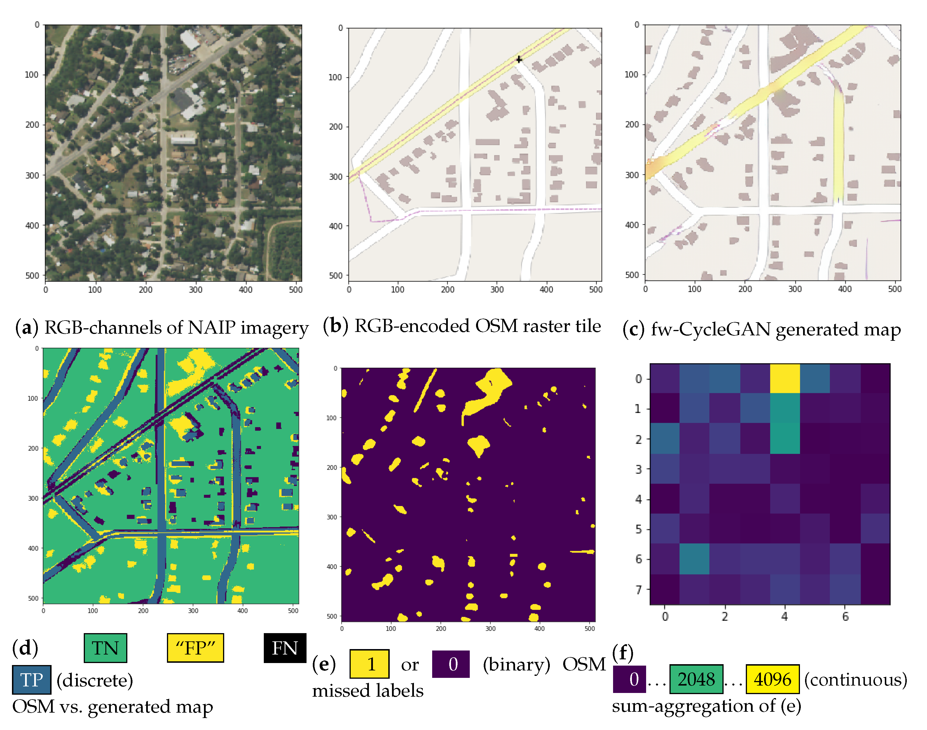
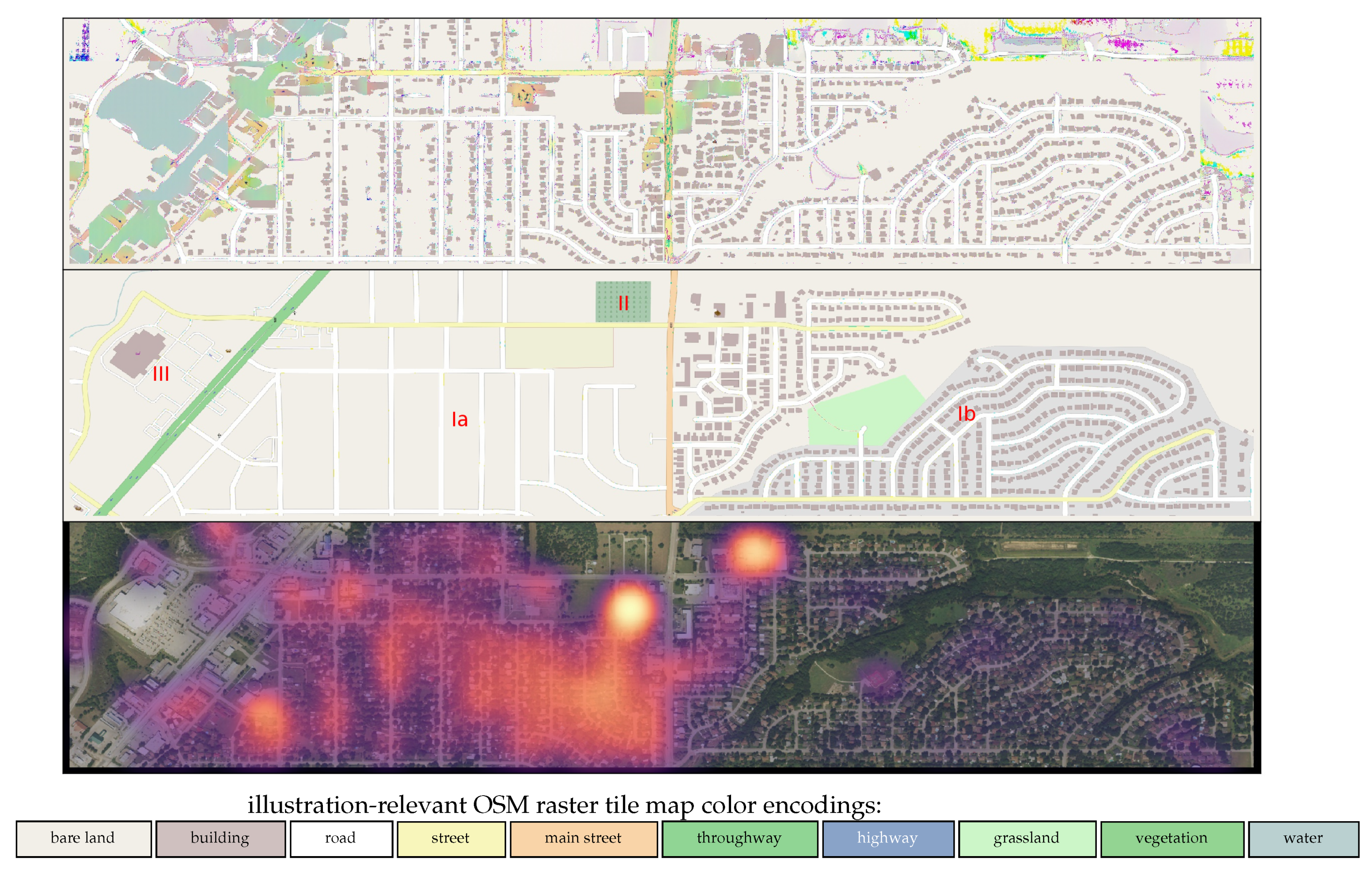
• Given the OSM map tiles, it is apparent that in the middle of the figure, Region b has residential house labels, while Region a has not yet been labeled by OSM mappers. Given NAIP data from 2016, the fw-CycleGAN is capable of identifying homes in Region a such that the technique presented in Figure 3 revealed a heat map with an indicative signal. Spurious magnitudes in Region b stemmed from imprecise georeferencing of buildings in the OSM map, as well as the vegetation cover above rooftops in the aerial NAIP imagery.
  Referring back to Listing 1, we had to allow for small color value variation with magnitude $2·$1 = 2 regarding the RGB feature color for buildings in the rasterized OSM map M. Thus, our approach became tolerant to minor perturbations in the map background other than bare land ((R,G,B) = (242,239,233), cf. sandy color in Region a) such as the grayish background in Region b needs to be accounted for. Similarly, a wider color-tolerance range of $2·$9 = 18 was set for the generated map $\widehat{M}$, which was noisier. Moreover, as we will discuss in Figure 5, we observed that the fw-CycleGAN tried to interpolate colors smoothly based on the feature’s context.
• fw-CycleGAN correctly identified roads and paths in areas where OSM had simply a park/recreational area marker. However, for the heat map defined by Listing 1, we restricted the analysis of the generated map $\widehat{M}$ to houses only—which was why the change in the road network in this part of the image was not reflected by the heat map.
• This section of the image demonstrated the limits of our current approach. In the generated map, colors were fluctuating wildly, while patches of land were marked as bodies of water (blue) or forestry (green). Further investigation is required if these artifacts were the result of idiosyncratic features in the map scarcely represented in the training dataset. We are planning to train on significantly larger datasets to answer this question.
  Another challenge of our current approach was exhibited by more extensive bodies of water. Though not present in Figure 4, we noticed the vertical aerial image-to-map ANN of the fw-CycleGAN to generate complex compositions of patches in such areas. Nevertheless, the heat map generated by the procedure outlined in Section 3.2 did not develop a pronounced signal that could potentially mislead OSM mappers. Thus, there were no false alarms due to these artifacts; regardless, an area to be labeled could be potentially missed in this way.

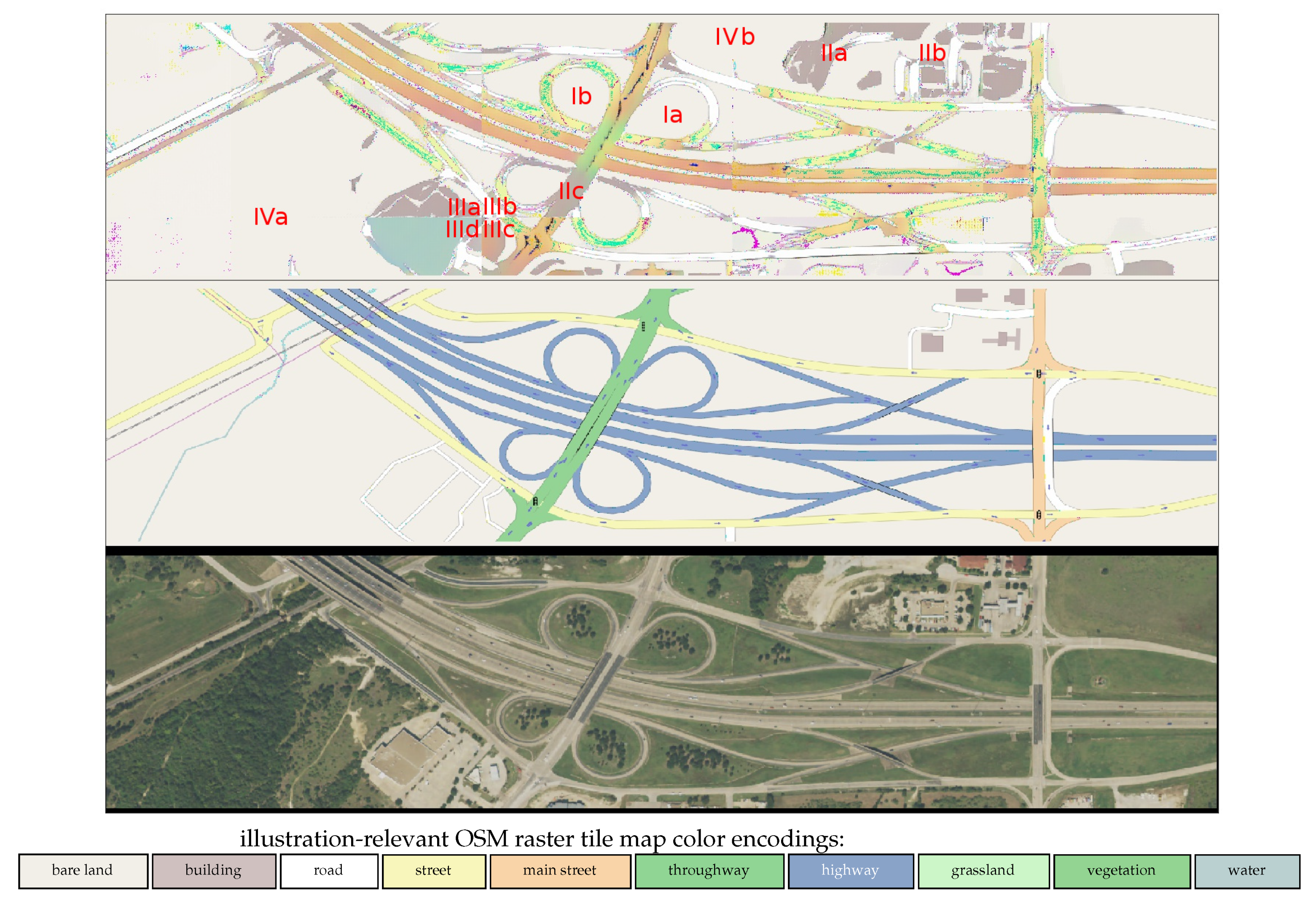
4.2. Change of Road Hierarchy from Color Interpolation

We turn our focus to road networks now. In contrast to buildings, streets have a hierarchical structure in OSM. The OSM map tile generator code assigns various colors to roads based on their position in this hierarchy. Figure 5, center plot, prominently illustrates the scenario for a motorway junction with exits to local streets in blue, green, yellow, orange, and white.

Let us elaborate on this kind of “change detection” concerning color interpolation of OSM sub-features labeled by different RGB values of the corresponding pixelated OSM map tiles:

• We begin by focusing on the circular highway exits. As apparent from the illustration, the fw-CycleGAN attempted to interpolate gradually from a major highway to a local street instead of assigning a discontinuous boundary.
• For our experiments, the feature weighting of the CycleGAN’s consistency loss was restricted to roads and buildings. Based on visual inspection of our training dataset of cities in Texas, we observed that rooftops (in particular, those of commercial buildings) and roads could share a similar sandy to grayish color tone. This might be the root cause why on inference, the typical brown color of OSM house labels became mixed into the road network, as clearly visible in Region c. Indeed, Regions a and b seemed to support such a hypothesis. More specifically, roads leading into a flat, extended, sandy parking lot area (as in Region a) might be misinterpreted as flat rooftops of, e.g., a shopping mall or depot, as in Region IIIa and IIId.
• In general, the context seemed to play a crucial role for inference: Where Regions a to d met, sharp transitions in color patches were visible. The generated map was obtained from stitching 512 × 512 pixel image mosaics without overlap. The interpretation of edge regions was impacted by information displayed southwest, northwest, northeast, and southeast of it. Variations could lead to a substantially different interpretation. Without proof, it might be possible that the natural scene southwest of Region d induced the blueish (water body) tone on the one hand, while, in contrast, the urban scene northeast of Region a triggered the alternating brown (building) and white (local road) inpainting on the other hand.
• Finally, Regions a and b provided a hallmark of our feature-weighting procedure. Although the NAIP imagery contained extended regions of vegetation, the fw-CycleGAN inferred bare ground.

The above considerations call for a deeper, more quantitative understanding of the CycleGAN architectures when it is being utilized as a translator from vertical aerial imagery to maps. Training on bigger sets of data might shed light on whether or not more diverse scenes help the network to refine scene understanding. However, there is conceptual-, network-, and training design-relevant questions as well. More studies along the lines of [67] are needed for a clear understanding of the inference of CycleGAN-type architectures for robust computational pipelines in practice.

5. Conclusions and Perspectives

In summary, this work highlighted the OSM label generation by image-to-image translation of vertical aerial photographs into rasterized OSM map tiles through deep neural networks. Table 1 presented quantitative measures of accuracy with respect to building detection for two different ANN architectures. First, transferring a trained ANN model from one geographic area to another impacted the overall accuracy of the detection. Secondly, manual inspection revealed that the overall accuracy of the model could be skewed by incomplete OSM labeling. Based on this insight, in another recent work, we developed an iterative scheme to retrain the ANN given its prediction from previous training runs [10].

Moreover, we elaborated on how to leverage the big geo-spatial data platform IBM PAIRS to generate heat maps that bear the potential of drawing OSM mapper’s attention to regions that might miss sufficient labeling. We demonstrated and qualitatively discussed the approach for building (change) detection and shared insight on how color-encoded road hierarchies (local road vs. highway) could highlight a change in road type employing the fw-CycleGAN for the vertical aerial imagery-to-map translation task.

Our work intended to serve as an interdisciplinary contribution to stimulate further research in the area of artificial intelligence (AI) for OSM data generation. Naturally, its success depended on the availability of free, high-resolution vertical aerial imagery. Although extrapolating the trajectory of spatial resolutions of globally available satellite imagery indicated that the OSM community might have to wait until the 2040s for this approach, governmental programs such as NAIP might enable it on a country-by-country basis already.

As a next step, it will be useful to test the viability of our methodology on medium resolution satellite imagery such as those from the Sentinel-2 mission. Furthermore, our approach of image-to-image translation is not limited to the RGB channels of vertical aerial imagery. Part of our future research agenda is to exploit LiDAR measurement as another source for high-resolution information on the centimeter scale from which false-RGB channels of various elevation models can be constructed for map generation by the fw-CycleGAN.

6. Patents

A U.S. patent on the feature-weighted training methodology of segmenting satellite imagery with the fw-CycleGAN has been submitted [83]. A distantly related patent that identifies and delineates vector data for (agricultural) land use is [84]. The IBM PAIRS technology is, e.g., protected by patent [85]. Among others, the patent application [86] details the overview layer generation that was used here to generate the change detection heat maps. Other patents exist protecting the IBM PAIRS platform. They are not directly related to this work.

References

1. OpenStreetMap. Available online: https://www.openstreetmap.org/ (accessed on 25 June 2020).
2. OpenStreetMap Editor. Available online: https://www.openstreetmap.org/edit (accessed on 25 June 2020).
3. He, K.; Gkioxari, G.; Dollár, P.; Girshick, R. Mask R-CNN. In Proceedings of the IEEE International Conference on Computer Vision, Venice, Italy, 22–29 October 2017; pp. 2961–2969. [Google Scholar] [CrossRef]
4. Badrinarayanan, V.; Kendall, A.; Cipolla, R. Segnet: A Deep Convolutional Encoder-Decoder Architecture for Image Segmentation. IEEE Trans. Pattern Anal. Mach. Intell. 2017, 39, 2481–2495. [Google Scholar] [CrossRef]
5. SegNet. Available online: https://mi.eng.cam.ac.uk/projects/segnet/ (accessed on 25 June 2020).
6. Isola, P.; Zhu, J.Y.; Zhou, T.; Efros, A.A. Image-to-Image Translation with Conditional Adversarial Networks. In Proceedings of the 2017 IEEE Conference on Computer Vision and Pattern Recognition (CVPR), Honolulu, HI, USA, 21–26 July 2017; pp. 5967–5976. [Google Scholar] [CrossRef] [Green Version]
7. Image-to-Image Translation with Conditional Adversarial Networks. Available online: https://phillipi.github.io/pix2pix/ (accessed on 25 June 2020).
8. Ronneberger, O.; Fischer, P.; Brox, T. U-Net: Convolutional Networks for Biomedical Image Segmentation. In Proceedings of the International Conference on Medical Image Computing and Computer-Assisted Intervention, Munich, Germany, 5–9 October 2015; pp. 234–241. [Google Scholar]
9. Schmidhuber, J. Unsupervised Minimax: Adversarial Curiosity, Generative Adversarial Networks, and Predictability Minimization. arXiv 2019, arXiv:cs/1906.04493. [Google Scholar]
10. Zhang, R.; Albrecht, C.; Zhang, W.; Cui, X.; Finkler, U.; Kung, D.; Lu, S. Map Generation from Large Scale Incomplete and Inaccurate Data Labels. arXiv 2020, arXiv:2005.10053. [Google Scholar]
11. Zhu, J.Y.; Park, T.; Isola, P.; Efros, A.A. Unpaired Image-to-Image Translation Using Cycle-Consistent Adversarial Networks. In Proceedings of the IEEE International Conference on Computer Vision, Venice, Italy, 22–29 October 2017; pp. 2242–2251. [Google Scholar] [CrossRef] [Green Version]
12. CycleGAN Project Page. Available online: https://junyanz.github.io/CycleGAN/ (accessed on 25 June 2020).
13. Tiecke, T.G.; Liu, X.; Zhang, A.; Gros, A.; Li, N.; Yetman, G.; Kilic, T.; Murray, S.; Blankespoor, B.; Prydz, E.B.; et al. Mapping the World Population One Building at a Time. arXiv 2017, arXiv:cs/1712.05839. [Google Scholar]
14. Iglovikov, V.; Seferbekov, S.S.; Buslaev, A.; Shvets, A. TernausNetV2: Fully Convolutional Network for Instance Segmentation. In Proceedings of the Conference on Computer Vision and Pattern Recognition Workshops (CVPRW), Salt Lake City, UT, USA, 18–22 June 2018; Volume 233, p. 237. [Google Scholar]
15. Microsoft/USBuildingFootprints. Available online: https://github.com/microsoft/USBuildingFootprints (accessed on 25 June 2020).
16. Albert, A.; Kaur, J.; Gonzalez, M.C. Using convolutional networks and satellite imagery to identify patterns in urban environments at a large scale. In Proceedings of the 23rd ACM SIGKDD International Conference on Knowledge Discovery and Data Mining, Halifax, NS, Canada, 13–17 August 2017; pp. 1357–1366. [Google Scholar]
17. Rakhlin, A.; Davydow, A.; Nikolenko, S.I. Land Cover Classification from Satellite Imagery with U-Net and Lovasz-Softmax Loss. In Proceedings of the Conference on Computer Vision and Pattern Recognition Workshops (CVPRW), Salt Lake City, UT, USA, 18–22 June 2018; pp. 262–266. [Google Scholar]
18. Cao, R.; Zhu, J.; Tu, W.; Li, Q.; Cao, J.; Liu, B.; Zhang, Q.; Qiu, G. Integrating aerial and street view images for urban land use classification. Remote Sens. 2018, 10, 1553. [Google Scholar] [CrossRef] [Green Version]
19. Kuo, T.S.; Tseng, K.S.; Yan, J.W.; Liu, Y.C.; Wang, Y.C.F. Deep Aggregation Net for Land Cover Classification. In Proceedings of the Conference on Computer Vision and Pattern Recognition Workshops (CVPRW), Salt Lake City, UT, USA, 18–22 June 2018; pp. 252–256. [Google Scholar]
20. Zhou, L.; Zhang, C.; Wu, M. D-LinkNet: LinkNet with Pretrained Encoder and Dilated Convolution for High Resolution Satellite Imagery Road Extraction. In Proceedings of the 2018 IEEE/CVF Conference on Computer Vision and Pattern Recognition Workshops (CVPRW), Salt Lake City, UT, USA, 18–22 June 2018; pp. 192–1924. [Google Scholar] [CrossRef]
21. Oehmcke, S.; Thrysøe, C.; Borgstad, A.; Salles, M.A.V.; Brandt, M.; Gieseke, F. Detecting Hardly Visible Roads in Low-Resolution Satellite Time Series Data. arXiv 2019, arXiv:1912.05026. [Google Scholar]
22. Buslaev, A.; Seferbekov, S.S.; Iglovikov, V.; Shvets, A. Fully Convolutional Network for Automatic Road Extraction From Satellite Imagery. In Proceedings of the Conference on Computer Vision and Pattern Recognition Workshops (CVPRW), Salt Lake City, UT, USA, 18–22 June 2018; pp. 207–210. [Google Scholar]
23. Xia, W.; Zhang, Y.Z.; Liu, J.; Luo, L.; Yang, K. Road extraction from high resolution image with deep convolution network—A case study of GF-2 image. In Multidisciplinary Digital Publishing Institute Proceedings; MDPI: Basel, Switzerland, 2018; Volume 2, p. 325. [Google Scholar]
24. Wu, S.; Du, C.; Chen, H.; Xu, Y.; Guo, N.; Jing, N. Road Extraction from Very High Resolution Images Using Weakly labeled OpenStreetMap Centerline. ISPRS Int. J. Geo-Inf. 2019, 8, 478. [Google Scholar] [CrossRef] [Green Version]
25. Xia, W.; Zhong, N.; Geng, D.; Luo, L. A weakly supervised road extraction approach via deep convolutional nets based image segmentation. In Proceedings of the 2017 International Workshop on Remote Sensing with Intelligent Processing (RSIP), Shanghai, China, 19–21 May 2017; pp. 1–5. [Google Scholar]
26. Sun, T.; Di, Z.; Che, P.; Liu, C.; Wang, Y. Leveraging crowdsourced gps data for road extraction from aerial imagery. In Proceedings of the IEEE Conference on Computer Vision and Pattern Recognition, Long Beach, CA, USA, 16–20 June 2019; pp. 7509–7518. [Google Scholar]
27. Ruan, S.; Long, C.; Bao, J.; Li, C.; Yu, Z.; Li, R.; Liang, Y.; He, T.; Zheng, Y. Learning to generate maps from trajectories. In Proceedings of the AAAI Conference on Artificial Intelligence, New York, NY, USA, 7–8 February 2020. [Google Scholar]
28. Liu, M.Y.; Breuel, T.; Kautz, J. Unsupervised image-to-image translation networks. In Advances in Neural Information Processing Systems; Curran Associates, Inc.: Red Hook, NY, USA, 2017; pp. 700–708. [Google Scholar]
29. Bonafilia, D.; Gill, J.; Basu, S.; Yang, D. Building High Resolution Maps for Humanitarian Aid and Development with Weakly-and Semi-Supervised Learning. In Proceedings of the IEEE Conference on Computer Vision and Pattern Recognition Workshops, Long Beach, CA, USA, 16–20 June 2019; pp. 1–9. [Google Scholar]
30. Singh, S.; Batra, A.; Pang, G.; Torresani, L.; Basu, S.; Paluri, M.; Jawahar, C. Self-Supervised Feature Learning for Semantic Segmentation of Overhead Imagery. In Proceedings of the The British Machine Vision Conference, Newcastle upon Tyne, UK, 3–6 September 2018; British Machine Vision Association: Durham, UK, 2018. [Google Scholar]
31. Ganguli, S.; Garzon, P.; Glaser, N. Geogan: A conditional gan with reconstruction and style loss to generate standard layer of maps from satellite images. arXiv 2019, arXiv:1902.05611. [Google Scholar]
32. Machine Learning—OpenStreetMap Wiki. Available online: https://wiki.openstreetmap.org/wiki/Machine_learning (accessed on 25 June 2020).
33. IBM PAIRS—Geoscope. Available online: https://ibmpairs.mybluemix.net/ (accessed on 25 June 2020).
34. Klein, L.; Marianno, F.; Albrecht, C.; Freitag, M.; Lu, S.; Hinds, N.; Shao, X.; Rodriguez, S.; Hamann, H. PAIRS: A scalable geo-spatial data analytics platform. In Proceedings of the 2015 IEEE International Conference on Big Data (Big Data), Santa Clara, CA, USA, 29 October–1 November 2015; pp. 1290–1298. [Google Scholar] [CrossRef]
35. Lu, S.; Freitag, M.; Klein, L.J.; Renwick, J.; Marianno, F.J.; Albrecht, C.M.; Hamann, H.F. IBM PAIRS Curated Big Data Service for Accelerated Geospatial Data Analytics and Discovery. In Proceedings of the 2016 IEEE International Conference on Big Data (Big Data), Washington, DC, USA, 5–8 December 2016; p. 2672. [Google Scholar] [CrossRef]
36. Albrecht, C.M.; Bobroff, N.; Elmegreen, B.; Freitag, M.; Hamann, H.F.; Khabibrakhmanov, I.; Klein, L.; Lu, S.; Marianno, F.; Schmude, J.; et al. PAIRS (re)loaded: System design and benchmarking for scalable geospatial applications. ISPRS Annals Proceedings 2020, in press. [Google Scholar]
37. Fecher, R.; Whitby, M.A. Optimizing Spatiotemporal Analysis Using Multidimensional Indexing with GeoWave. In Proceedings of the Free and Open Source Software for Geospatial (FOSS4G) Conference, Hyderabad, India, 26–29 January 2017; Volume 17, p. 10. [Google Scholar] [CrossRef]
38. Hughes, J.N.; Annex, A.; Eichelberger, C.N.; Fox, A.; Hulbert, A.; Ronquest, M. Geomesa: A Distributed Architecture for Spatio-Temporal Fusion. In Proceedings of the PIE 9473, Geospatial Informatics, Fusion, and Motion Video Analytics V, Baltimore, MD, USA, 20–24 April 2015; SPIE: Bellingham, WA, USA, 2015. [Google Scholar]
39. Whitman, R.T.; Park, M.B.; Ambrose, S.M.; Hoel, E.G. Spatial indexing and analytics on Hadoop. In Proceedings of the 22nd ACM SIGSPATIAL International Conference on Advances in Geographic Information Systems, Dallas, TX, USA, 4–7 November 2014; Association for Computing Machinery: New York, NY, USA, 2014. [Google Scholar]
40. Albrecht, C.M.; Fisher, C.; Freitag, M.; Hamann, H.F.; Pankanti, S.; Pezzutti, F.; Rossi, F. Learning and Recognizing Archeological Features from LiDAR Data. In Proceedings of the 2019 IEEE International Conference on Big Data (Big Data), Los Angeles, CA, USA, 9–12 December 2019; pp. 5630–5636. [Google Scholar] [CrossRef] [Green Version]
41. Klein, L.J.; Albrecht, C.M.; Zhou, W.; Siebenschuh, C.; Pankanti, S.; Hamann, H.F.; Lu, S. N-Dimensional Geospatial Data and Analytics for Critical Infrastructure Risk Assessment. In Proceedings of the 2019 IEEE International Conference on Big Data (Big Data), Los Angeles, CA, USA, 9–12 December 2019; pp. 5637–5643. [Google Scholar] [CrossRef]
42. Elmegreen, B.; Albrecht, C.; Hamann, H.; Klein, L.; Lu, S.; Schmude, J. Physical Analytics Integrated Repository and Services for Astronomy: PAIRS-A. Bull. Am. Astron. Soc. 2019, 51, 28. [Google Scholar]
43. Vora, M.N. Hadoop-HBase for Large-Scale Data. In Proceedings of the 2011 International Conference on Computer Science and Network Technology, Harbin, China, 24–26 December 2011; Volume 1, pp. 601–605. [Google Scholar] [CrossRef]
44. Home—Spatial Reference. Available online: https://spatialreference.org/ (accessed on 25 June 2020).
45. Janssen, V. Understanding Coordinate Reference Systems, Datums and Transformations. Int. J. Geoinform. 2009, 5, 41–53. [Google Scholar]
46. Samet, H. The Quadtree and Related Hierarchical Data Structures. ACM Comput. Surv. 1984, 16, 187–260. [Google Scholar] [CrossRef] [Green Version]
47. Drusch, M.; Del Bello, U.; Carlier, S.; Colin, O.; Fernandez, V.; Gascon, F.; Hoersch, B.; Isola, C.; Laberinti, P.; Martimort, P.; et al. Sentinel-2: ESA’s optical high-resolution mission for GMES operational services. Remote. Sens. Environ. 2012, 120, 25–36. [Google Scholar] [CrossRef]
48. Roy, D.P.; Wulder, M.A.; Lovel, T.R.; Woodcock, C.E.; Allen, R.G.; Anderson, M.C.; Helder, D.; Irons, J.R.; Johnson, D.M.; Kennedy, R.; et al. Landsat-8: Science and Product Vision for Terrestrial Global Change Research. Remote. Sens. Environ. 2014, 145, 154–172. [Google Scholar] [CrossRef] [Green Version]
49. Landsat Missions Webpage. Available online: https://www.usgs.gov/land-resources/nli/landsat/landsat-satellite-missions (accessed on 25 June 2020).
50. Terra Mission Webpage. Available online: https://terra.nasa.gov/about/mission (accessed on 25 June 2020).
51. Sentinel-2 Mission Webpage. Available online: https://sentinel.esa.int/web/sentinel/missions/sentinel-2 (accessed on 25 June 2020).
52. Lim, K.; Treitz, P.; Wulder, M.; St-Onge, B.; Flood, M. LiDAR Remote Sensing of Forest Structure. Prog. Phys. Geogr. 2003, 27, 88–106. [Google Scholar] [CrossRef] [Green Version]
53. Meng, X.; Currit, N.; Zhao, K. Ground Filtering Algorithms for Airborne LiDAR Data: A Review of Critical Issues. Remote. Sens. 2010, 2, 833–860. [Google Scholar] [CrossRef] [Green Version]
54. Soergel, U. (Ed.) Radar Remote Sensing of Urban Areas, 1st ed.; Book Series: Remote Sensing and Digital Image Processing; Springer: Heidelberg, Germany, 2010. [Google Scholar] [CrossRef]
55. Ouchi, K. Recent Trend and Advance of Synthetic Aperture Radar with Selected Topics. Remote. Sens. 2013, 5, 716–807. [Google Scholar] [CrossRef] [Green Version]
56. Naip Data in Box. Available online: https://nrcs.app.box.com/v/naip (accessed on 25 June 2020).
57. USGS EROS Archive—Aerial Photography—National Agriculture Imagery Program (NAIP). Available online: https://0-doi-org.brum.beds.ac.uk/10.5066/F7QN651G (accessed on 28 June 2020).
58. WMF Labs Tile Server: “OSM No Labels”. Available online: https://tiles.wmflabs.org/osm-no-labels/ (accessed on 25 June 2020).
59. OSM Server: “Tiles with Labels”. Available online: https://tile.openstreetmap.de/ (accessed on 25 June 2020).
60. Rezatofighi, H.; Tsoi, N.; Gwak, J.; Sadeghian, A.; Reid, I.; Savarese, S. Generalized Intersection Over Union: A Metric and a Loss for Bounding Box Regression. In Proceedings of the 2019 IEEE/CVF Conference on Computer Vision and Pattern Recognition (CVPR), Long Beach, CA, USA, 16–20 June 2019; pp. 658–666. [Google Scholar] [CrossRef] [Green Version]
61. Pytorch/Pytorch. Available online: https://github.com/pytorch/pytorch (accessed on 25 June 2020).
62. milesial. Milesial/Pytorch-UNet. Available online: https://github.com/milesial/Pytorch-UNet (accessed on 25 June 2020).
63. Zhu, J.Y. Junyanz/Pytorch-CycleGAN-and-Pix2pix. Available online: https://github.com/junyanz/pytorch-CycleGAN-and-pix2pix (accessed on 25 June 2020).
64. Mapnik/Mapnik. Available online: https://github.com/mapnik/mapnik (accessed on 25 June 2020).
65. IBM/Ibmpairs. Available online: https://github.com/IBM/ibmpairs (accessed on 25 June 2020).
66. IBM PAIRS—Tutorial. Available online: https://pairs.res.ibm.com/tutorial/ (accessed on 25 June 2020).
67. Chu, C.; Zhmoginov, A.; Sandler, M. CycleGAN, a Master of Steganography. arXiv 2017, arXiv:1712.02950. [Google Scholar]
68. Deng, J.; Dong, W.; Socher, R.; Li, L.J.; Li, K.; Li, F.-F. ImageNet: A Large-Scale Hierarchical Image Database. In Proceedings of the 2019 IEEE/CVF Conference on Computer Vision and Pattern Recognition (CVPR), Long Beach, CA, USA, 16–20 June 2019; pp. 248–255. [Google Scholar] [CrossRef] [Green Version]
69. ImageNet. Available online: http://www.image-net.org/ (accessed on 25 June 2020).
70. Van Etten, A.; Lindenbaum, D.; Bacastow, T.M. SpaceNet: A Remote Sensing Dataset and Challenge Series. arXiv 2018, arXiv:1807.01232. [Google Scholar]
71. SpaceNet. Available online: https://spacenetchallenge.github.io/ (accessed on 25 June 2020).
72. Winning Solution for the Spacenet Challenge: Joint Learning with OpenStreetMap. Available online: https://i.ho.lc/winning-solution-for-the-spacenet-challenge-joint-learning-with-openstreetmap.html (accessed on 25 June 2020).
73. Powers, D.M. Evaluation: From Precision, Recall and F-Measure to ROC, Informedness, Markedness and Correlation; Bioinfo Publications: Pune, India, 2011. [Google Scholar]
74. Pan, S.J.; Yang, Q. A Survey on Transfer Learning. IEEE Trans. Knowl. Data Eng. 2009, 22, 1345–1359. [Google Scholar] [CrossRef]
75. Lu, J.; Behbood, V.; Hao, P.; Zuo, H.; Xue, S.; Zhang, G. Transfer Learning Using Computational Intelligence: A Survey. Knowl. Based Syst. 2015, 80, 14–23. [Google Scholar] [CrossRef]
76. Weiss, K.; Khoshgoftaar, T.M.; Wang, D. A Survey of Transfer Learning. IEEE Trans. Knowl. Data Eng. 2009, 3, 9. [Google Scholar] [CrossRef] [Green Version]
77. Lin, J.; Jiang, Z.; Sarkaria, S.; Ma, D.; Zhao, Y. Special Issue Deep Transfer Learning for Remote Sensing. Remote Sensing (Journal). Available online: https://0-www-mdpi-com.brum.beds.ac.uk/journal/remotesensing/special_issues/DeepTransfer_Learning (accessed on 28 June 2020).
78. Xie, M.; Jean, N.; Burke, M.; Lobell, D.; Ermon, S. Transfer Learning from Deep Features for Remote Sensing and Poverty Mapping. In Proceedings of the AAAI 2016: Thirtieth AAAI Conference on Artificial Intelligence, Phoenix, AZ, USA, 12–17 February 2016; p. 7. [Google Scholar]
79. Huang, Z.; Pan, Z.; Lei, B. Transfer Learning with Deep Convolutional Neural Network for SAR Target Classification with Limited Labeled Data. Remote. Sens. 2017, 9, 907. [Google Scholar] [CrossRef] [Green Version]
80. Lian, X.; Zhang, C.; Zhang, H.; Hsieh, C.J.; Zhang, W.; Liu, J. Can Decentralized Algorithms Outperform Centralized Algorithms? A Case Study for Decentralized Parallel Stochastic Gradient Descent. In Advances in Neural Information Processing Systems 30; Guyon, I., Luxburg, U.V., Bengio, S., Wallach, H., Fergus, R., Vishwanathan, S., Garnett, R., Eds.; Curran Associates, Inc.: Red Hook, NY, USA, 2017; pp. 5330–5340. [Google Scholar]
81. Zhang, W.; Cui, X.; Kayi, A.; Liu, M.; Finkler, U.; Kingsbury, B.; Saon, G.; Mroueh, Y.; Buyuktosunoglu, A.; Das, P.; et al. Improving Efficiency in Large-Scale Decentralized Distributed Training. In Proceedings of the ICASSP 2020 IEEE International Conference on Acoustics, Speech and Signal Processing (ICASSP), Barcelona, Spain, 4–8 May 2020. [Google Scholar]
82. Bing Maps. Available online: https://www.bing.com/maps (accessed on 25 June 2020).
83. Zhang, R.; Albrecht, C.M.; Freitag, M.; Lu, S.; Zhang, W.; Finkler, U.; Kung, D.S.; Cui, X. System and Methodology for Correcting Map Features Using Remote Sensing and Deep Learning. U.S. Patent. application submitted, under review.
84. Klein, L.J.; Lu, S.; Albrecht, C.M.; Marianno, F.J.; Hamann, H.F. Method and System for Crop Recognition and Boundary Delineation. U.S. Patent 10445877B2, 15 October 2019. [Google Scholar]
85. Klein, L.; Marianno, F.J.; Freitag, M.; Hamann, H.F.; Rodriguez, S.B. Parallel Querying of Adjustible Resolution Geospatial Database. U.S. Patent 10372705B2, 6 August 2019. [Google Scholar]
86. Freitag, M.; Albrecht, C.M.; Marianno, F.J.; Lu, S.; Hamann, H.F.; Schmude, J.W. Efficient Querying Using Overview Layers of Geospatial—Temporal Data in a Data Analytics Platform. U.S. Patent P201805207, 14 May 2020. [Google Scholar]
87. Mapnik.Org—the Core of Geospatial Visualization and Processing. Available online: https://mapnik.org/ (accessed on 25 June 2020).
88. Wikimedia Cloud Services Team. Available online: https://www.mediawiki.org/wiki/Wikimedia_Cloud_Services_team (accessed on 25 June 2020).
89. Bottou, L.; Curtis, F.E.; Nocedal, J. Optimization Methods for Large-Scale Machine Learning. Siam Rev. 2018, 60, 223–311. [Google Scholar] [CrossRef]
90. Nwankpa, C.; Ijomah, W.; Gachagan, A.; Marshall, S. Activation Functions: Comparison of Trends in Practice and Research for Deep Learning. arXiv 2018, arXiv:1811.03378. [Google Scholar]
91. Shi, W.; Caballero, J.; Theis, L.; Huszar, F.; Aitken, A.; Ledig, C.; Wang, Z. Is the Deconvolution Layer the Same as a Convolutional Layer? arXiv 2016, arXiv:1609.07009. [Google Scholar]
92. Kingma, D.P.; Welling, M. An Introduction to Variational Autoencoders. arXiv 2019, arXiv:1906.02691. [Google Scholar] [CrossRef]
93. Kurach, K.; Lučić, M.; Zhai, X.; Michalski, M.; Gelly, S. A Large-Scale Study on Regularization and Normalization in GANs. In Proceedings of the International Conference on Machine Learning, Long Beach, CA, USA, 9–15 June 2019. [Google Scholar]
94. Hinton, G.E.; Srivastava, N.; Krizhevsky, A.; Sutskever, I.; Salakhutdinov, R.R. Improving Neural Networks by Preventing Co-Adaptation of Feature Detectors. arXiv 2012, arXiv:1207.0580. [Google Scholar]
95. Ioffe, S.; Szegedy, C. Batch Normalization: Accelerating Deep Network Training by Reducing Internal Covariate Shift. arXiv 2015, arXiv:1502.03167. [Google Scholar]
96. Bengio, Y.; Louradour, J.; Collobert, R.; Weston, J. Curriculum Learning. In Proceedings of the 26th Annual International Conference on Machine Learning—ICML ’09, Montreal, QC, Canada, 14–18 June 2009; pp. 1–8. [Google Scholar] [CrossRef]
97. Parisi, G.I.; Kemker, R.; Part, J.L.; Kanan, C.; Wermter, S. Continual Lifelong Learning with Neural Networks: A Review. Neural Netw. 2019, 113, 54–71. [Google Scholar] [CrossRef] [PubMed]
Figure 1. Naive extrapolation for the increase of spatial resolution r > 0 over time t for publicly available satellite imagery with global coverage.
Ijgi 09 00427 g001
Figure 2. IBM PAIRS data and processing workflow for OSM change detection heat map generation. Dashed boxes represent data sources and sinks, and solid boxes encapsulate processing units. The right-hand side column of aligned (colored) raster grids serves as a cartoon of nested geospatial indexing in IBM PAIRS.
Ijgi 09 00427 g002
Figure 3. Illustration of data processing for change detection in OSM data from aerial imagery visualized for the combined human infrastructure features of buildings and road networks. The top row depicts samples of the raw data of our study, Figure 3a,b, and the resulting generated map, Figure 3c, from the fw-CycleGAN. Figure 3d illustrates the pixel labeling of the fw-CycleGAN versus the OSM ground truth as follows: TP—OSM and the fw-CycleGAN agree on the existence of human infrastructure (true positive); TN—both OSM and the fw-CycleGAN do not indicate human infrastructure (true negative); FP—the fw-CycleGAN identifies human infrastructure missed by OSM (“false positive”); Note: We use quotation marks, because a significant fraction of FP pixels are TP; as is obvious from the ground truth satellite image, Figure 3a; FN—OSM labels human infrastructure missed by the fw-CycleGAN (false negative); Figure 3e reduces Figure 3d by showing “false positives” (numerical pixel value 1), only, on a (numerical pixel value 0).
Ijgi 09 00427 g003
Figure 4. OSM change detection heat map for buildings. The plot depicts a residential area in the southwest suburbs of Dallas. The upper plot shows the map inferred by the trained fw-CycleGAN; the plot in the middle hosts the OSM map tiles without text; and the lower strip illustrates the RGB representation of NAIP imagery overlayed by the inferred heat map (cf Figure 3f) of change detection for buildings—a key result of this work. Red labels Ia, Ib, II, and III in the middle panel serve as guidance for the eyes for the discussion in the main text. We vertically aligned three plots of the same spatial extent.
Ijgi 09 00427 g004
Figure 5. Road hierarchy change detection from OSM color encoding. The figure shows a highway junction with exits located north of the residential area discussed in Figure 4. The upper panel shows the map inferred from the trained fw-CycleGAN; the plot in the middle hosts the OSM map tiles without text; and the lower strip shows the NAIP imagery.
Ijgi 09 00427 g005