High Resolution Viewscape Modeling Evaluated Through Immersive Virtual Environments

Abstract

Visual characteristics of urban environments influence human perception and behavior, including choices for living, recreation and modes of transportation. Although geospatial visualizations hold great potential to better inform urban planning and design, computational methods are lacking to realistically measure and model urban and parkland viewscapes at sufficiently fine-scale resolution. In this study, we develop and evaluate an integrative approach to measuring and modeling fine-scale viewscape characteristics of a mixed-use urban environment, a city park. Our viewscape approach improves the integration of geospatial and perception elicitation techniques by combining high-resolution lidar-based digital surface models, visual obstruction, and photorealistic immersive virtual environments (IVEs). We assessed the realism of our viewscape models by comparing metrics of viewscape composition and configuration to human subject evaluations of IVEs across multiple landscape settings. We found strongly significant correlations between viewscape metrics and participants’ perceptions of viewscape openness and naturalness, and moderately strong correlations with landscape complexity. These results suggest that lidar-enhanced viewscape models can adequately represent visual characteristics of fine-scale urban environments. Findings also indicate the existence of relationships between human perception and landscape pattern. Our approach allows urban planners and designers to model and virtually evaluate high-resolution viewscapes of urban parks and natural landscapes with fine-scale details never before demonstrated.

1. Introduction

The visual characteristics of landscapes, such as complexity, openness, and naturalness, are known to be linked to people’s perceptions and behaviors [1,2,3,4,5,6]. These characteristics—expressed, e.g., by quantity and variety of visible landcover or by variations in surface elevation—have been previously analyzed from landscape photographs [3,4,5,6] providing reliable, detailed information about the local survey sites [7]. The effort to extend the analysis over larger areas has led to GIS approaches that are easy to automate, but may be viewed as less realistic [8,9,10,11,12,13,14]. For example, viewshed analyses of areas visible from a given vantage point [10,11,12] have been used as a way to link mapping with the visible landscape [9,13,14]. Conceptualized as viewscape modeling, researchers are beginning to characterize visible landscape content, such as land use or surface greenness, to better understand visual connections between people and their surroundings [15,16]. Analysis of viewscape composition can be extended by computing the spatial configuration of visible landscapes (e.g., pattern diversity [17], shape complexity [18], terrain ruggedness [19]) using landscape metrics from the field of landscape ecology. Viewscapes based on digital surface models (DSM), rather than previously used digital terrain models (DTMs), include vertical structures, such as buildings and vegetation and are less likely to overestimate viewscape area [16]. Where horizontal visibility is important, such as in urban settings, they may still incompletely represent the visible area and its associated characteristics (e.g., Reference [20]). Application of viewscape models to understand the visual characteristics of finer-scale features in urban environments remains largely unexplored. In contrast to more commonly studied biomes, such as pasture and forest, that can include large vistas and fairly homogenous landcover (e.g., References [21,22,23]), urban landscapes involve a variety of view ranges and spatial conditions—shaped through the interaction of granular landforms and heterogeneous built environments.

Limitations of spatial scale exist for both DSM and landcover data that are integral to the realistic estimation of visible content (e.g., number of visible trees and buildings), as well as for the accuracy of landscape metric analysis (reviewed in References [24,25]). Publicly available landcover data are often coarse (10–30 m) and do not represent features smaller than their pixel size (e.g., buildings, sidewalks, single trees). Although advanced methods, such as object-based classification or pattern recognition, exist to generate highly detailed landcover data from satellite imagery, incorporation of such data in viewscape models has been rare [11]. Difficulties in the accessibility of lidar data—the most common DSM data source—have caused most current viewscape models to use low-resolution DSMs or DTMs [18]. This is in spite of the well-documented influence of spatial data resolution on the accuracy of visibility analysis [9,16,26]. Coarser DSMs tend to overestimate visibility compared to fine-grained lidar DSMs, especially in smaller viewsheds [26]. However, lidar-sourced DSMs may still struggle to realistically represent non-surface vegetation (Figure 1). Specifically, raster-based DSMs represent trees as solid protrusions that entirely obscure the under-canopy and through canopy visibility [27,28]. This is a major source of error for visibility estimations, particularly within the dense canopy (parks and greenways), or in leaf-off season when visibility through deciduous trees is computed. Several techniques have been proposed to overcome this issue, such as the visual permeability concept that accounts for the probability of viewing a region as determined by the spatial density and position of tree models [29], or trunk obstruction modeling that replaces the trees with an approximated trunk model [28]. While improvements in resolution of spatial data and vegetation obstruction modeling have separately shown promise in enhancing the accuracy of visibility analysis, to our knowledge, they have not been used together in a single study to generate a high fidelity viewscape model.

Evaluating the extent to which a viewscape model can predict perceived visual characteristics requires a comparison of the model output with human subjects’ evaluations of landscape, which could be done either in situ or through landscape photography and 3D simulations. Because in situ measurements are often time-consuming, labor-intensive and involve several confounding factors (e.g., changing weather), research has widely resorted to online or desktop surveys using photographs and 3D simulations [18]. However, the use of digital stimuli is increasingly contested for their representation validity, with the least realism reported for photographs of heterogeneous landscapes and mixed-use urban environments [7]. Another obstacle for verification of viewscape models is the discrepancy of view coverage between perspective photographs and visibility analysis in GIS. Perspective photographs have a limited field of view (FOV), while viewshed algorithms use 360° line-of-sight algorithms to calculate visibility for the entire horizontal and vertical FOV. Immersive virtual environments (IVEs) that immerse the observer in a virtual environment (VE) can potentially minimize the gap between modeled viewscape and in situ experience of the urban landscape. In contrast to desktop displays where FOVs are limited, immersive displays (CAVE or head-mounted displays, HMD) provide continuous visual feedback linked to the user’s head and body orientation allowing them to freely explore the entire viewshed area. Thanks to the ability of IVEs to elicit a higher sense of immersion [30], presence [31], and improved spatial perceptions (e.g., distance, depth) [32]. IVEs have been widely adopted in geospatial sciences and urban planning applications, such as 3D visualization of open map data [33], real-time 3D visualization of ecological simulations [34], and geodesign [35]. However, to our knowledge, IVE has not been used for human verification of visibility simulations, particularly viewscape modeling.

The purpose of this study is to develop and evaluate a high-resolution approach to measuring and modeling fine-scale viewscape characteristics of mixed-use urban environments through a novel integration of geospatial and perception elicitation techniques using photorealistic IVEs. We use high-resolution DSM and landcover data derived from lidar to account for the fine-grained structure and heterogeneous patterns of urban environments, and we improve the vegetation visibility of the DSM using trunk obstruction modeling. With these improved spatial data, we compute viewscape composition and configuration using automated GIS procedures. We uniquely evaluate the realism of the resultant viewscape model by quantifying its capacity to predict perceived visual characteristics. For this, we conduct a perception survey using IVE images captured from a set of locations across the study area. Then we compare the metrics of viewscape composition and configuration derived from the viewscape model with human subject evaluations of IVEs.

We specifically focus on three visual characteristics, namely, visual access, complexity, and naturalness that have been widely used to objectively measure visual landscape quality and have shown to be strongly linked with human psychological responses to environments [1,36,37,38,39,40,41]. By bridging the gap between objective and subjective analysis of visual characteristics, our high-resolution viewscape modeling allows landscape designers and planners to realistically simulate aesthetic and restorative qualities of a viewscape in a spatially explicit manner.

2. Methods

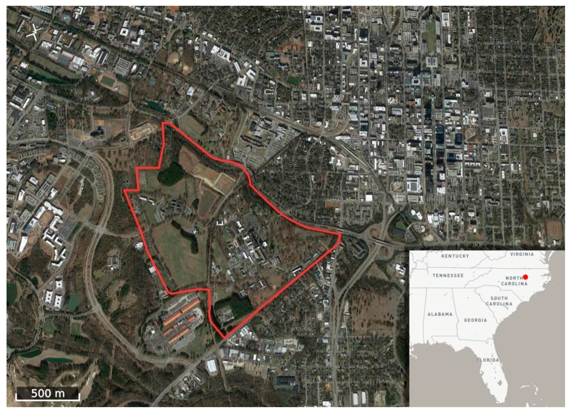
2.1. Study area

Dorothea Dix urban park covers 306 acres (125 ha) in Raleigh, North Carolina (35’46° N, 78’39° W; Figure 2). The landscape is characterized by undulating topography and heterogeneous landcover. Vegetation cover ranges from grassy meadows, herbaceous perennials, Eastern and Loblolly pines, Willow and Red Eastern oaks, and a variety of landscaping trees and shrubs. As a past psychiatric hospital campus, the site includes numerous buildings, including closed hospital, administrative and maintenance buildings and derelict employee housing, as well as a network of paved roads (dixpark.org). Some buildings are currently being used by the NC Department of Health and Human Services. The combination of varied landscape types and spatial characteristics provides a wide range of conditions of openness, complexity, and naturalness, making the selected site well-suited for the purposes of this study.

2.2. Viewscape Modeling

To model urban viewscapes, we first develop DSM and a high-resolution landcover map. Then, we improve the visibility of viewscapes calculated from DSM using enhanced vegetation modeling accounting for visibility under the deciduous tree crowns. Finally, we represent fine-scale visual characteristics of features in a mixed-use urban environment by measuring the composition and configuration of viewscapes.

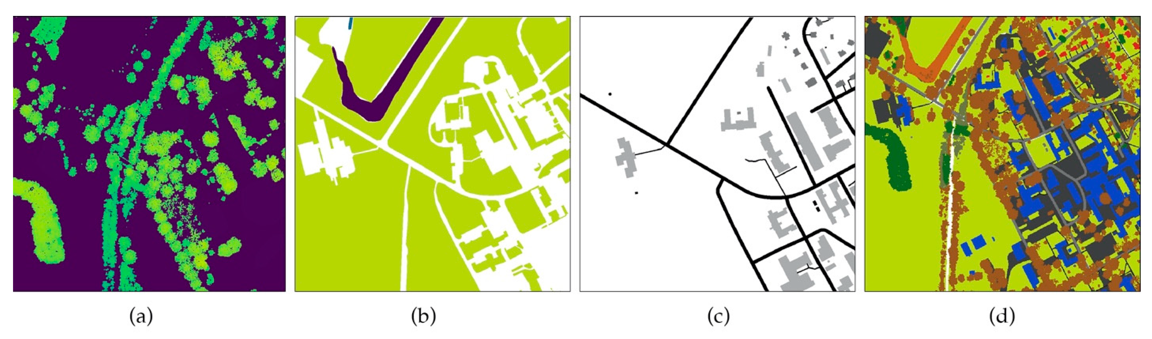
2.2.1. Digital Surface Model (DSM) and Landcover

To develop the DSM and landcover map, we used three geospatial datasets, including airborne lidar, multi-spectral orthoimagery of vegetation and road and building vector data. The multiple return lidar data were acquired on 11 January 2015 (leaf-off) with an average density of 2 points/m² and fundamental vertical accuracy (FVA) of 18.2 cm (Phase 3–2015 NC QL2 lidar, https://sdd.nc.gov/). The lidar point cloud was classified by data provider into several classes, including ground and low, medium, and high vegetation. Two sets of orthoimagery were used: a 30 cm resolution orthoimagery captured in early 2015 in leaf-off condition (WMS, 2015), and a 1 m resolution four-band imagery captured in summer 2014 in leaf-on condition (NAIP, USDA Farm Services Agency, 2014).

DSM was developed by interpolating first-return lidar points at half-meter resolution. We used a regularized spline with tension algorithm implemented in GRASS GIS [42] to balance the smoothness and approximation accuracy of the surface. The landcover was developed by combining the three layers (Figure 3):

• Canopy height model (CHM) was, obtained through filtering and interpolating lidar vegetation points and subtracting their elevation from ground elevation (Figure 3a). We applied a supervised classification method [43] to strata of infrared imagery (NAIP), lidar vegetation maximum values, and orthoimagery to classify the CHM into the mixed forest, evergreen and deciduous landcovers (Figure 3b).
• The ground cover layer consists of grasslands, herbaceous, and unpaved surfaces, which were manually digitized in the 30 cm resolution orthoimagery.
• Buildings and paved surfaces (e.g., streets, parking surface), which were rasterized from the vector line and polygon data (Figure 3c; data retrieved from City of Raleigh GIS datasets; Raleigh, NC, US Open Data server, https://data-ral.opendata.arcgis.com/).

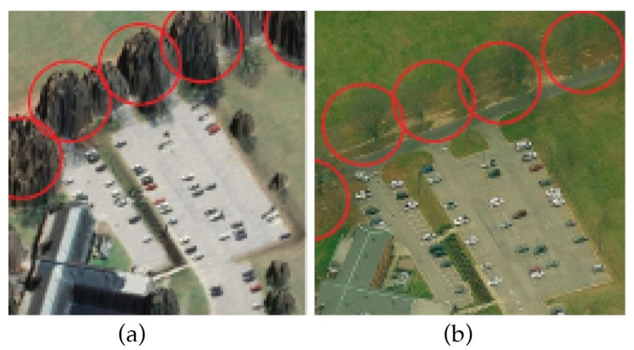
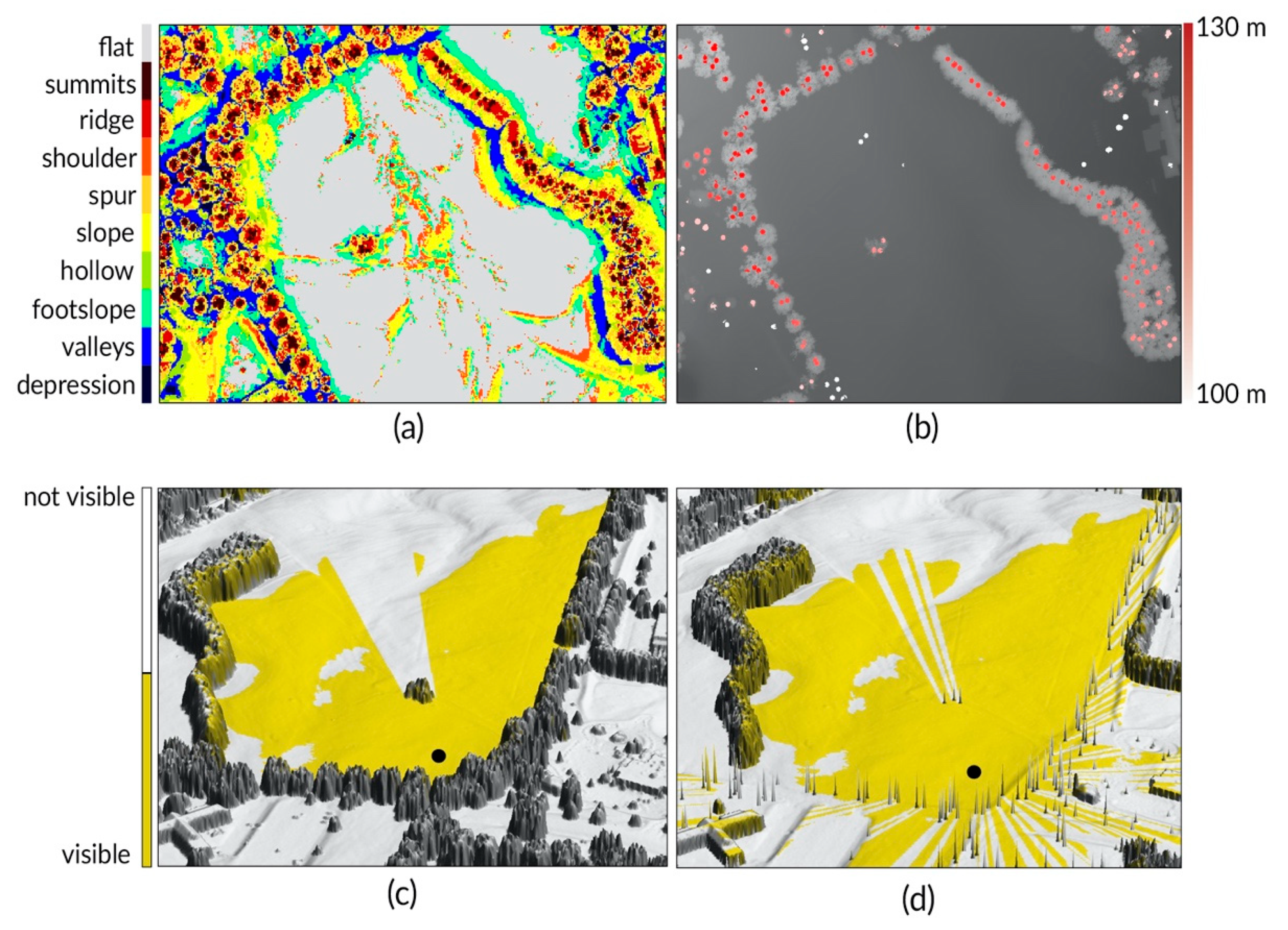
2.2.2. Trunk Obstruction Modeling

To delineate vegetation structures that affect visibility, we visually inspected lidar points and field images and identified three main structures (Figure 4): (a) Dense evergreen patches (mainly Loblolly pines) with dense understory (mainly woody shrubs and vines), (b) evergreen over-story mixed with deciduous midstory (mainly red maple and sweetgum) and understory, and (c) dispersed deciduous species consisting of large willow and Northern red oaks, maples and landscaping trees. While the former two structures were mostly or entirely impenetrable, the third structure had substantial under-canopy and through-canopy visibility in the leaf-off condition.

To overcome the visibility error of the deciduous canopies, we used the trunk obstruction modeling method suggested by Murgoitio [28] that has been shown to significantly improve short-range visibility estimations. The method involves delineating individual trees from the lidar point cloud, and substituting them in the DSM with approximate trunk width measures. To do this, we delineated the individual treetops from the DSM using Geomorphons [44]—an algorithm that uses pattern recognition principles to detect and classify landforms in an elevation model (Figure 5a). Geomorphons can accurately detect treetops of deciduous and coniferous stands within complex forest structures [45]. We extracted the summits from the classified landform raster map (0.5 m resolution) to delineate treetop polygons and used their centroids to designate the location and height of the tree trunk. We assumed that the apex of the canopy corresponded with the trunk location on a straight vertical line to the terrain. Based on field measurements and spatial resolution of the data, we used a diameter of 1 m for larger species (oaks) and a 0.5 m diameter for smaller species. Finally, the deciduous canopies in the DSM were replaced with the segmented trunks to create the improved surface model.

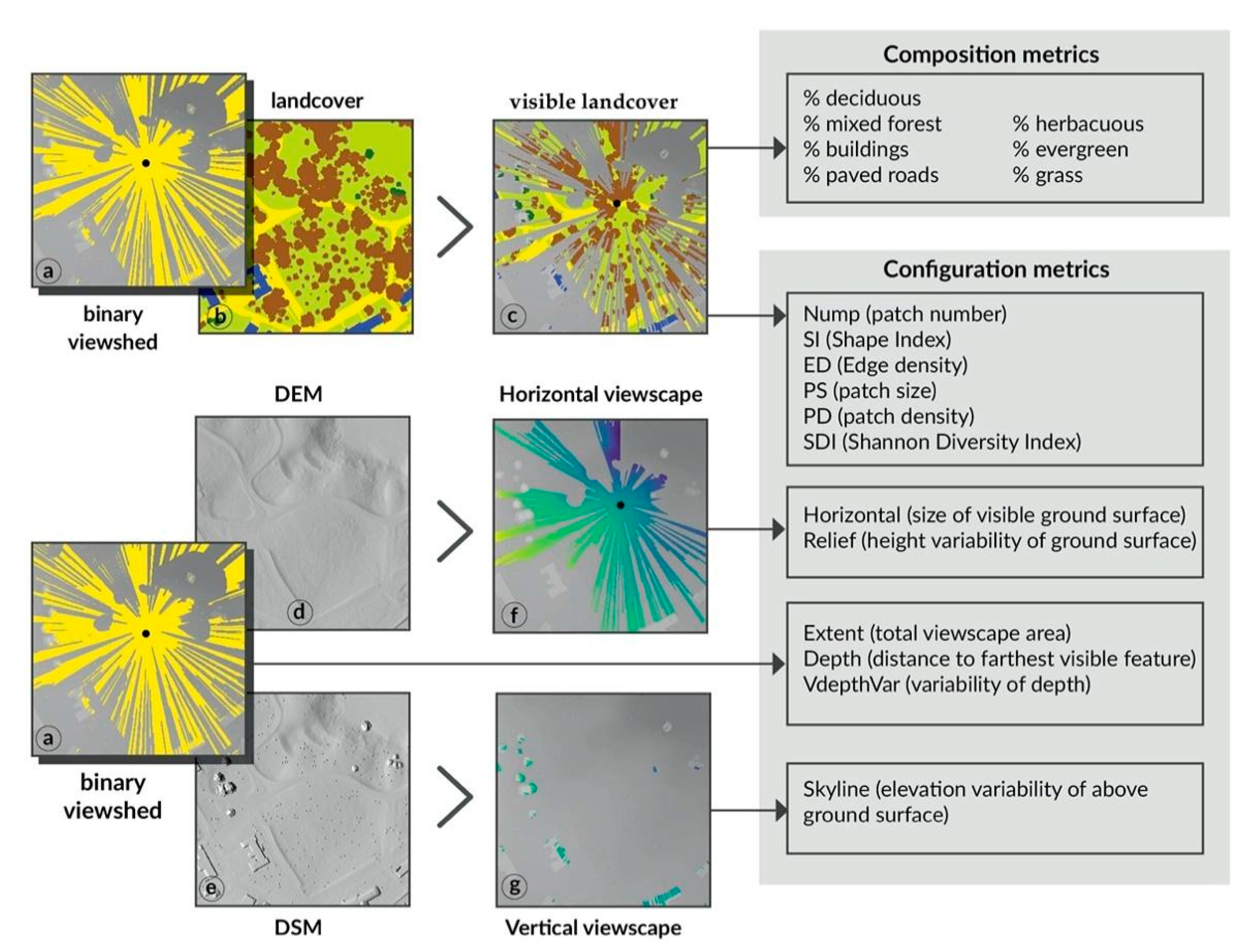
2.2.3. Computing Viewscape Metrics

To obtain the viewscape metrics, we measured the composition and configuration of viewscapes computed from 342 viewpoints (centroids of a 30 m grid) across the study area. Thus, we assumed an observer every 30 m across the site to be able to represent the visual characteristics of the site. Viewsheds were computed on the DSM at average human eye-level (1.65 m) and considered a maximum visibility distance of 3000 m, based on viewing range estimated by a preliminary viewshed analysis. We used the GRASS GIS viewshed function, which uses a computationally-efficient line-sweeping algorithm suitable for performing viewshed computation on a high-resolution DSM [16,46]. The algorithm rotates a sweep line around the observer cell and determines the visibility of each cell when the sweep line passes over its center.

Computed viewscape metrics consisted of 19 landscape indicators that represent visual characteristics and are previously shown to predict human perceptions and landscape preferences [18]. Composition metrics characterize the visual content of a viewscape and quantify what landscape features an observer can see from a given vantage point [18,47]. To compute these metrics, we intersected the binary (visible or nonvisible) viewshed map (Figure 5a) with landcover map (Figure 5b) to obtain a visible landcover map (Figure 5c) from which we calculated the proportional presence of each landcover in the viewscape.

Configuration metrics measure the spatial arrangement and relationship between different landcover types. They included (1) total viewscape area (extent), (2) distance to the farthest visible feature (depth), (3) elevation variability of the visible ground surface (relief), (4) elevation variability of the visible above-ground features (skyline), (5) size of the visible ground surface (horizontal), (6) variability of depth (VdepthVar), (7) number of patches (Nump), (8) complexity of patch shapes (SI and ED), (9) size of patches (PS), (10) patches density (PD), and (11) land type diversity measured as Shannon’s diversity index (SDI). Depth and extent were computed directly from the binary viewshed map (Figure 5a). To compute horizontal, relief and skyline metrics, the viewshed map was intersected with a bare-earth DEM (Figure 5d) and DSM (Figure 5e) to develop separate maps of ground visibility (horizontal viewscape; Figure 5f) and aboveground visibility (vertical viewscape; Figure 5g), respectively. The remaining metrics (Nump, SI, ED, PS, PD, and SDI) were derived from visible landcover map (Figure 5c) and measured using landscape metrics analysis [48]. The definition of the variables and calculation formulas are described below.

Shannon diversity index (SDI) is a measure of pattern diversity by considering the number of land cover classes and the proportion of distribution. Higher SDI values indicate an increase in the number of classes or even distribution, or both. It can be computed as follows, where i is patch type, m is the number of different patch types and p_i is the proportional abundance of patch type i:

$$SDI=-{\displaystyle \sum }_{i=1}^m p_{i }ln\left(p_{i }\right)$$

(1)

Shape index (SI) characterizes visible patchiness based on perimeter-to-area ratio where E is sum of all patch edges, and A is sum of all patch areas. Lower shape complexity indicates more coherent views.

$$SI=\frac{0.25E}{\sqrt{A}}$$

(2)

Edge density (ED) provides a measurement of the length of the edge segments per hectare and is dependent on both patchiness and patch shape. A high value would indicate a low degree of variation between the largest and smallest patch. E is the sum of the lengths of all edge segments, and A is total landscape area:

$$ED=\frac{E}{A}\left(\mathrm{10,000}\right)$$

(3)

The number of patches (Nump) describes the number of patches in the landscape and explains the extent to which the landscape is fragmented or not. Higher values of Nump indicate a more fragmented arrangement. Patch size (PS) is the average size of patches over the entire viewscape area with a lower value indicating a more granular composition of a view. Patch density (PD) is the number of patches per area. A higher value indicates greater heterogeneity and decreased coherence of landscape.

The entire GIS analysis and automation workflow (Figure 5), was performed via a python script in GRASS GIS (can be found in Supplementary Materials).

2.3. Immersive Virtual Environment (IVE) Survey of Perceived Visual Characteristics

To verify the realism of the viewscape model and evaluate its capacity to predict perceived visual characteristics, we conduct a survey of perceived visual characteristics using IVE stimuli representing a range of urban viewscapes in the study area. Below, we describe the process for selection of viewpoint locations and the procedure for creating IVE scenes from photographs collected from these viewpoints, and then explain the details of the survey procedure.

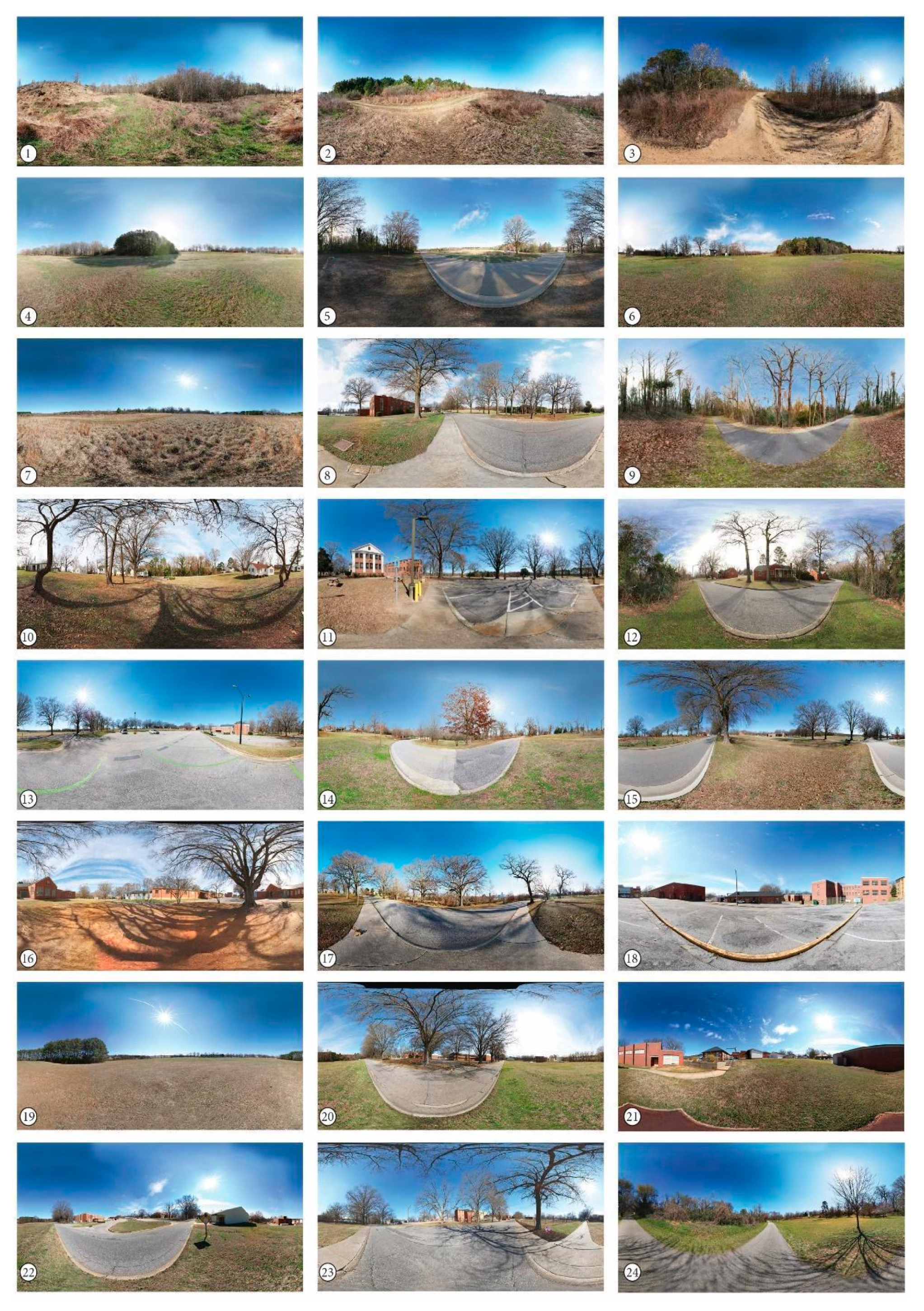
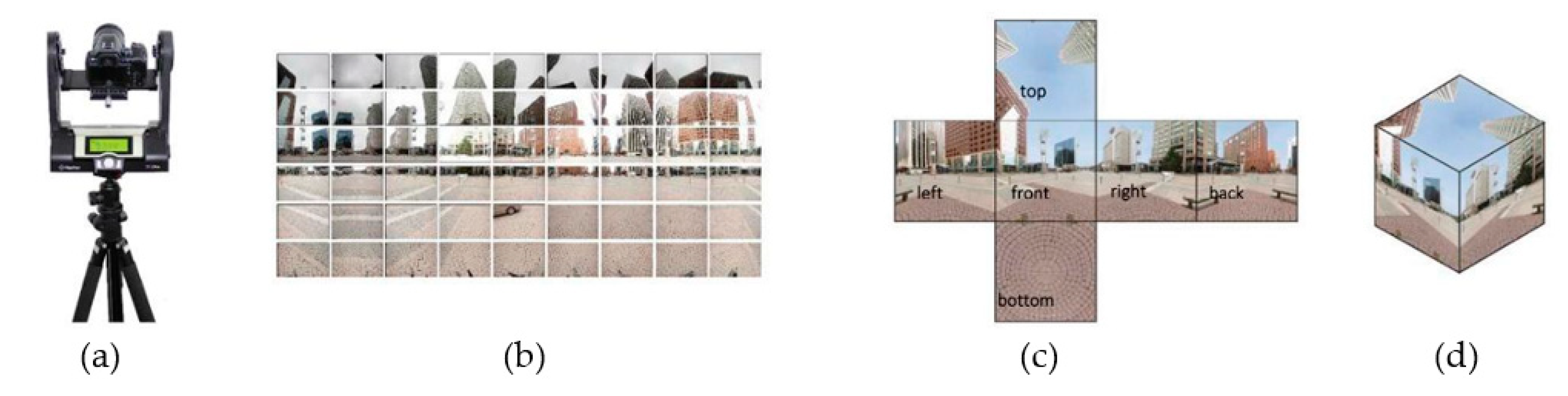
2.3.1. IVE Stimuli

To select viewpoints for model verification we assessed the viewscape metrics using two criteria: (1) The visual attributes of the selected viewpoints should approximately represent the range of values of the 342 viewpoints; and (2) viewpoints should be at least two grid cells (60 m) apart to ensure that the entire study area is represented. A sample of 24 points satisfied these criteria, and was considered for acquiring photographs (Figure 6).

Viewpoints were located using a handheld GPS device (Trimble Geo5t). At each location, we took an array of 54 (9 × 6) photographs, at eye-level (1.65 m), using a Canon Eos 70D camera fixed on a robotic mount (Gigapan Epic Pro; Figure 7). We stitched the images to acquire a 25 Megapixel panoramic image with a spherical projection, i.e., equirectangular image (Figure 7b). Then, through a process known as cube mapping [49], each equirectangular image was unfolded into six cube faces (Figure 7c). In a virtual reality set-up, these faces are wrapped as a cubic environment around the viewer (Figure 7d). Photographs were taken over four days in February 2017, in similar weather and lighting conditions.

2.3.2. Survey Procedure

In total, 100 undergraduate students at a university in the southeastern United States participated in this study. The mean age among the participants was 19.56 years (SD = 3.17); 51% were male (n = 51) and 70% were white (n = 70). Participants’ study background varied; 47% were from parks recreation and tourism management, 25% from sports management and 28% from natural and social sciences. Participation in the study was voluntary, and those who volunteered were entered in a random drawing for one of the ten $25 gift cards to an online merchant. The study protocol was approved by the university’s Institutional Review Board.

To measure perceived visual characteristics, we selected three items that have shown strong links with human psychological responses. Perceived visual access (also called visual scale), broadly defined as size, shape, diversity, and degree of openness of the landscape, is shown to have links with perceived safety [36] and preference [41]. It was measured using one question without explicit reference to openness: “How well can you see all parts of this environment without having your view blocked or interfered with?” [46]. The response options ranged from 0 = not at all to 10 = very easy. Perceived naturalness, defined as the extent to which landscape is close to a perceived natural state [40,50], which correlates with perceived restoration [37] and stress recovery [38]. It was measured by a single question “How natural do you perceive this environment?” using an 11-point scale with 0 = not natural, 10 = very natural [51]. For perceived complexity—important in the formation of visual preference [1,39,52]—participants responded to the statement “How complex you perceive this environment? “using an 11-point scale, 0 = not at all, 10 = very complex [53].

The IVE survey was carried out in a controlled lab environment. Upon participants’ arrival, a researcher assisted them to don and adjust head-mounted display (HMD) (Oculus CV1), practice rotating around, and interacting with the joystick controller. To familiarize participants with experience of immersion and respond to an on-screen survey, they experienced two mockup IVE scenes depicting an urban plaza and a park. For each scene, they responded to three statements measuring perceived realism and presence in the virtual environment.

After the warmup phase, each respondent experienced 24 randomly displayed IVEs with a 2-min recess after the 12th scene. Each of the IVE scenes was to be rated on only one of the response variables (perceived visual access, perceived complexity, and perceived naturalness) and the variable for the rating was randomly selected by the VR application at the start of the study. Final sample sizes were 32 for ‘visual access,’ 34 for ‘naturalness’, and 34 for ‘complexity.’ Administering all three questions to participants would have increased our statistical power, but our pilot study (n = 11) showed that responding to multiple questions for each IVE can lead to participants’ fatigue and confusion. By doing so, we also avoided the carryover bias, that is the possible impact of previous questions on the subsequent ones [54].

Participants experienced each scene for 25 s, after which, a semi-transparent dialogue box containing the survey item was displayed on the HMD. There was no time limitation in the response phase allowing respondents to freely explore the immersive environment and rate the statement (using the joystick controller) as they continued to experience the scene. The entire experiment procedure was developed as a python script and executed in World Vizard VR development software (WorldViz Inc, Version 5.4).

Following the experimental session, participants filled-out a brief pen-and-paper survey, including questions about age, race, gender, and field of study. The total duration of each session was on average 40 min (range 37–46). Data were collected over four weeks in March 2017.

2.4. Viewscape Model Assessment

We used multiple linear regression analyses to assess how the viewscape model represented by 19 viewscape metrics predicts three perceived visual characteristics, namely, perception of visual access, perception of complexity, and perception of naturalness. Our study had a within-subjects design, meaning that each participant experienced all 24 scenes (or plots) and responded only to one of the three dependent variables. As such, the unit of analysis was the participant’s rating of a scene. Three separate stepwise variable selection models based on the minimization of the Akaïke Information Criterion (AIC) were applied to fit the best predictive model for each dependent variable. For each of the regression models, we diagnosed collinearity using the variance inflation factor (VIF) to include variables with a tolerance of larger than 0.1 and VIF smaller than 10, as suggested by Hair et al. [55]. The prediction power of regression models are reported using adjusted coefficients of determination (R²_adj), and the relative contribution of each variable to the model is reported using standardized regression coefficients.

3. Results

3.1. Viewscape Modeling

The resulting landcover map (Figure 8) developed by combining CHM, digitized high-resolution orthoimagery and official datasets of roads and building footprints had a 0.5 m resolution and included eight landcover classes categorized based on the National Landcover Dataset (NLCD) classification. By applying Geomorphons algorithm (Figure 9a) on the interpolated high-resolution DSM, we successfully identified treetops (Figure 9b) and based on the landcover substituted the deciduous trees in the DSM with their trunks. Figure 9c,d demonstrate the improvement of short-range visibility estimations by comparing the modeled viewscape before and after trunk obstruction modeling. We computed 19 viewscape metrics from 342 viewpoints distributed on a 30m grid across the study area. From these viewpoints we selected 24 locations that approximately represent the range of values of all the viewpoints with the condition to be distributed at least 60 m apart to represent the entire study area.

Table 1. Computed viewscape metrics for the 24 IVE scenes used in the study.

	Composition Metrics							Configuration Metrics
Viewscape	Deciduous	Mixed	Evergreen	Herbaceous	Grass	Building	Paved	extent	depth	relief	skyline	horizontal	VdepthVar	Nump	SI	ED	PS	PD	SDI
	(%)	(%)	(%)	(%)	(%)	(%)	(%)	(m2)	(m)	(m)	(m)	(m2)
1	4.40	28.60	0.40	66.10	0.00	0.40	0.00	6921	99	4.29	8.04	6904	4.13	3	18.31	6955	0.09	58,756	0.82
2	13.40	42.00	2.80	31.00	30.00	2.60	0.30	21,214	2130	6.78	1.86	2089	36.99	2	73.48	14,373	0.01	127,130	1.56
3	4.40	28.60	0.40	4.30	37.90	0.30	1.60	3140	506	11.10	4.65	1273	24.73	1	39.53	11,462	0.07	91,617	0.95
4	27.40	3.90	4.00	0.00	56.50	4.90	3.30	42,582	325	3.14	8.28	40,666	10.10	20	26.09	4186	0.04	33,455	1.22
5	7.30	8.10	7.10	6.30	56.50	3.30	2.80	98,618	812	4.44	10.55	79,819	18.28	82	47.52	4964	0.04	30,744	1.75
6	8.50	14.00	3.70	0.00	63.20	5.20	1.90	91,891	1972	5.91	9.38	61,032	16.85	21	49.44	5294	0.04	31,170	1.45
7	12.80	12.10	2.30	0.00	60.00	4.20	7.70	97,852	2132	5.97	11.20	68,717	18.67	27	48.02	5075	0.04	30,504	1.41
8	5.30	18.50	5.40	5.30	59.50	1.90	0.90	103,798	1789	3.40	9.58	55,347	14.99	73	54.37	5463	0.05	33,642	1.53
9	19.80	5.10	3.40	0.00	54.40	6.70	10.50	91,018	1074	5.37	11.37	60,146	29.40	73	53.24	5917	0.04	34,626	1.37
10	0.00	60.80	0.00	0.00	39.20	0.00	0.00	80	150	0.26	6.09	79	2.24	2	5.60	14,168	0.05	102,955	0.67
11	24.90	14.10	4.80	0.00	35.90	10.00	10.30	5593	366	2.37	10.08	5457	6.16	22	20.21	7676	0.09	56,625	1.68
12	10.80	16.20	7.70	0.00	43.80	10.70	8.60	36,353	982	3.17	9.28	22,770	19.82	18	49.59	7839	0.08	50,237	1.76
13	32.50	0.40	4.80	0.00	28.20	23.00	11.00	1712	210	2.22	10.20	1564	6.10	8	14.14	10,021	0.13	87,406	1.62
14	13.30	3.50	7.10	0.90	62.50	4.50	8.10	106,496	891	5.36	11.33	96,335	17.88	36	39.73	4081	0.03	21,146	1.27
15	25.60	25.20	2.80	0.00	34.40	5.20	6.80	19,282	461	5.36	10.71	16,813	11.50	19	42.10	8806	0.11	69,296	1.53
16	13.90	4.10	7.40	2.40	59.80	4.50	22.00	104,086	843	5.89	10.37	81,323	25.46	50	48.48	5098	0.04	30,592	1.37
17	22.30	5.80	0.20	0.00	16.70	22.70	32.40	8605	311	1.36	6.34	6409	7.37	17	18.63	5752	0.05	35,191	1.51
18	32.70	5.70	3.20	0.00	52.70	2.00	3.80	28,459	305	5.31	12.59	25,200	16.61	32	32.72	6298	0.05	42,796	1.20
19	26.30	22.20	1.30	0.00	35.00	3.90	11.20	50,713	1293	4.76	12.04	34,196	26.99	42	63.49	8672	0.08	59,631	1.52
20	7.40	2.90	10.30	0.00	12.60	18.10	48.80	10,702	300	2.11	6.22	10,369	5.29	13	19.73	5642	0.06	40,294	1.45
21	10.40	3.50	5.00	0.70	69.90	3.80	6.40	185,289	538	7.12	11.20	167,052	17.30	44	39.15	3109	0.02	17,501	1.11
22	24.20	5.30	8.70	0.00	46.00	5.80	10.00	42,773	325	2.93	7.90	38,522	12.37	31	33.13	5093	0.04	32,375	1.50
23	9.30	0.40	0.20	0.00	25.90	23.00	41.20	6250	137	1.10	7.26	6059	4.96	12	15.35	5425	0.06	43,198	1.31
24	23.00	3.00	7.20	0.00	28.90	15.30	22.70	23,569	414	1.55	7.02	21,166	17.10	23	37.48	7370	0.08	55,496	1.61

Variables: VdepthVar = view depth variation, Nump = patch number, ED = edge density, SI = shape index, ED = edge density, PS = patch size, PD = patch density, SDI = Shannon’s diversity index.

shows the computed values of both composition and configuration viewscape metrics for those 24 selected viewpoints.

3.2. Immersive Virtual Environment Survey

The mean values of perceived visual access of IVEs varied between 1.85 and 10.62 (

Table 2. Descriptive statistic of participants ratings of perceived visual access (n = 34), perceived naturalness (n = 32) and perceived complexity (n = 34) for the 24 IVE scenes used in the survey.

	Visual Access				Naturalness				Complexity
IVE Scene	Mean	SD	min	max	Mean	SD	min	max	Mean	SD	min	max
1	2.21	1.51	1.00	9.00	10.31	1.03	6.00	11.00	2.29	1.22	1.00	4.00
2	4.76	0.89	4.00	7.00	9.48	1.52	3.00	11.00	3.82	1.38	2.00	6.00
3	3.53	1.66	2.00	9.00	9.38	1.64	3.00	11.00	4.71	1.95	2.00	11.00
4	7.88	2.33	4.00	11.00	8.06	2.22	3.00	11.00	4.35	1.91	1.00	10.00
5	8.65	1.79	3.00	10.00	7.24	2.12	3.00	11.00	8.03	1.22	6.00	10.00
6	8.59	1.91	4.00	11.00	7.72	1.17	4.00	9.00	7.18	2.68	1.00	11.00
7	8.94	2.04	3.00	11.00	7.78	1.95	4.00	11.00	6.74	2.31	2.00	10.00
8	9.12	2.24	3.00	11.00	9.22	1.07	6.00	11.00	6.09	2.39	1.00	10.00
9	8.88	1.04	5.00	10.00	7.09	1.99	4.00	11.00	9.09	2.68	1.00	11.00
10	1.85	1.13	1.00	7.00	9.50	1.24	6.00	11.00	2.41	2.27	0.00	10.00
11	3.53	1.56	2.00	8.00	6.91	2.10	3.00	11.00	8.71	1.75	2.00	11.00
12	7.32	1.97	4.00	11.00	6.36	2.04	3.00	11.00	8.56	1.60	6.00	11.00
13	2.38	1.61	1.00	9.00	4.03	0.93	3.00	6.00	7.85	1.13	6.00	10.00
14	9.53	1.78	2.00	11.00	6.06	2.76	1.00	11.00	6.03	2.28	1.00	10.00
15	8.18	1.64	4.00	11.00	7.91	2.05	4.00	11.00	7.15	1.28	5.00	9.00
16	8.35	1.81	5.00	11.00	7.24	1.97	3.00	11.00	7.68	1.34	6.00	10.00
17	5.62	2.53	2.00	11.00	3.97	1.23	2.00	9.00	8.85	2.34	4.00	11.00
18	7.74	2.06	1.00	11.00	8.91	1.96	2.00	11.00	4.06	1.59	2.00	9.00
19	8.29	1.64	6.00	11.00	8.09	1.67	5.00	11.00	7.71	2.36	2.00	11.00
20	5.29	2.52	1.00	11.00	1.68	1.14	1.00	6.00	5.47	2.98	1.00	11.00
21	10.62	0.49	10.00	11.00	8.65	1.33	3.00	10.00	4.44	1.42	2.00	7.00
22	7.09	1.82	4.00	11.00	6.48	2.27	2.00	11.00	6.41	2.40	1.00	10.00
23	3.00	0.85	2.00	4.00	2.32	1.25	1.00	7.00	9.00	2.13	4.00	11.00
24	7.12	2.25	2.00	11.00	3.32	1.05	2.00	7.00	8.74	1.19	7.00	11.00

). Very high values were assigned to viewscapes with long vistas and large viewshed areas (scenes 21, 14), and viewscapes enclosed by forests, hills, and buildings (scenes 1, 10, 13) obtained the lowest values. The selected regression model for perceived visual access included 11 variables and produced an adjusted coefficient of determination (R²_adj) of 0.65, p < .001 (

Table 3. Multiple linear regression models for the three perceived visual characteristics, perceived visual access, perceived naturalness, and perceived complexity on viewscape metrics.

Perceived Visual Characteristic	Viewscape Metric	Coefficient	Normalized Coefficient	Student t	p		Tolerance	VIF
Perceived Visual Access	(Intercept)	7.120		7.11	<.001	***
	Extent	0.000	0.390	6.74	<.001	***	0.14	7.15
	Depth	0.001	0.110	2.94	.003	**	0.333	3
n = 32	Skyline	−0.176	−0.143	−2.76	.006	**	0.173	5.77
R² adj = 0.65	Relief	−0.158	−0.119	−2.85	.004	**	0.27	3.7
p < .001	Vdepth_var	0.077	0.215	3.94	<.001	***	0.157	6.36
	Building	−0.180	−0.414	−7.61	<.001	***	0.159	6.28
	Paved	0.026	0.106	2.21	.028	*	0.201	4.97
	Deciduous	0.058	0.173	4.65	<.001	***	0.338	2.96
	Herbaceous	−0.044	−0.20	−6.87	<.001	***	0.551	1.82
	Nump	19.200	0.164	3.17	.002	**	0.175	5.72
	ED	0.000	−0.390	−7.33	<.001	***	0.163	6.12
Perceived Naturalness
	(Intercept)	2.441		3.25	.001	**
	Relief	0.157	0.128	3.88	<.001	***	0.471	2.12
n = 34	Deciduous	0.057	0.187	6.30	<.001	***	0.582	1.72
R² adj = 0.62	Mixed	0.074	0.370	9.07	<.001	***	0.311	3.21
p < .001	Evergreen	−0.13	−0.133	−4.36	<.001	***	0.537	1.86
	Herbaceous	0.067	0.335	8.26	<.001	***	0.315	3.18
	Grass	0.066	0.407	7.25	<.001	***	0.164	6.11
	Building	−0.12	−0.302	−5.42	<.001	***	0.166	6.02
	SI	−0.017	−0.124	−3.19	.001	**	0.549	1.82
	Nump	7.026	0.102	2.08	.038	*	0.517	1.94
Perceived Complexity
	(Intercept)	−1.37		−3.47	<.001	***
	Relief	0.152	0.126	2.58	.008	**	0.549	1.82
n = 34	Depth	−0.001	−0.138	−2.95	.003	**	0.328	3.05
R² adj = 0.42	Skyline	0.06	0.072	1.59	.032	*	0.408	2.45
p < .001	Building	0.191	0.474	10.32	<.001	***	0.344	2.91
	SDI	2.74	0.305	7.88	<.001	***	0.442	2.26
	ED	0.001	0.142	3.36	<.001	***	0.367	2.73
	Nump	0.001	0.378	5.93	<.001	***	0.123	8.1

Variables: Vdepth_var = view depth variation, NUMP = patch number, ED = edge density, SI = shape index, SDI = Shannon’s diversity index. *** = p < .001; ** = p < .01; * p = < .05

). Extent had the strongest positive contribution to the model, followed by Viewdepth_var and Depth. Skyline and Relief, respectively, had a negative correlation with perceived visual access. From the compositional metrics, Building had a strong negative impact on perceived visual access, whereas Deciduous and Paved positively contributed to the model. Among configuration metrics, ED (edge density) had the strongest negative contribution to the model, while Nump (number of patches) was positively related to perceived visual access.

Perceptions of naturalness ranged from 1.68 and 10.31 (Table 2). Viewscapes depicting herbaceous landcover, mixed forests, and unpaved surfaces received highest ratings (scenes 1, 2, 3) and those within highly built areas with little vegetation coverage received the lowest ratings (scenes 20, 23). With a selection of nine variables, the regression model explained 62% of the variation in perceived naturalness (R²_adj = 0.62, p < .001). The majority of variation was explained by compositional metrics. Grass coverage had the highest positive correlation with perceived naturalness, followed by Mixed, Herbaceous and Deciduous coverage. A significant inverse correlation was found for Building. From the configuration metrics, Relief and Nump had positive contributions, and SI had a negative contribution to the model.

Perceptions of complexity varied from 2.29 to 9.09 (Table 2). The lowest values were assigned to viewscapes with lowest SDI (scenes 1, 10), whereas those with the highest SDI were perceived as highly complex. With a selection of seven visual attributes, the model explained 42% percent of the variation in perceived complexity (R²_adj = 0.42, p < 001). Most of the contribution came from configuration variables (Table 3). Among those, Nump had the highest positive impact, followed by SDI and ED. Relief and Skyline—measures of terrain and above-terrain vertical variability—both positively affected perceived complexity, while Depth had a negative correlation. From the composition metrics, relative Building coverage was the only and the most positively correlated variable with perceived complexity.

4. Discussion

The purpose of this study was to develop and evaluate a high-resolution approach to modeling fine-scale viewscape characteristics of mixed-use urban environments. We utilized high-resolution spatial data and improved vegetation modeling method to develop a viewscape model accounting for granularity and heterogeneity of mixed-use urban environments. Using human subject’s evaluations of IVEs taken from the study area, we assessed the capacity of the viewscape model to predict three perceived visual characteristics, namely, visual access, naturalness, and complexity. Our results show that with our proposed approach, viewscape models can reliably capture the visual characteristics of the urban park environments. Findings also confirm the relationships between landscape configuration and composition, and examined perceptions.

4.1. Predicting Perceived Visual Characteristics

Statistically, our viewscape models for perceived visual access, naturalness, and complexity provide results with good explanatory power. Regression models explain almost 65% of the variance in perceptions at best (naturalness, visual access) and as much as 45% at worst (complexity). These results are comparable to those in a similar analysis by Schirpke et al. [14] and Sahraoui et al. [18] that estimated perceptions of mountain regions and urban-rural fringes, respectively using viewscapes.

Regarding the metrics selected for the visual access model, the analysis shows that extent (viewshed size) and depth had a strong positive impact on the perceived visual access. This finding is in line with extant studies indicating that the observer’s distance between the obscuring elements (depth) and the amount of visible space (extent) have a strong influence on perceived visual access [41,56,57]. Depth variation—the spatial variation of the view depth [18]—also showed a positive impact on perceived access. This indicator is analogous with “number of perceptual rooms,” which is one of the main determinants of visual access, as found by Tveit [57]. An interesting finding concerns the strong negative role of buildings and the positive role of deciduous trees in perceived visual accessibility, emphasizing the importance of permeability (porosity) of the obscuring elements. Indeed, in leaf-off season deciduous forests allow for more visibility through the branches compared to evergreen and mixed forests. Similarly, horizontal surfaces occupy a smaller proportion of the visible landscape, unlike buildings whose vertical development leads to significant visual salience.

For perceived naturalness, we found a positive role played by green spaces and natural groundcover, such as grasslands and herbaceous landcover, which is consistent with what is generally reported in the literature. In contrast to previous studies that combined all forest typologies as a single forest landcover, incorporation of fine-grained landcover enabled our model to discriminate between forest types and revealed perception differences among them. Mixed forests consisting of more than two stand types and abundantly covered by mosses and lichens, were perceived as more natural than the deciduous and evergreen specimens, which parallels previous studies suggesting that less maintained and varied representation of vegetation positively impact perceived naturalness [2,57]. Also, as expected, human-made elements, such as residential or administrative buildings, had a negative effect on naturalness judgments. We also found a strong impact of Relief, indicating that viewscapes with a higher vertical variation or rugged terrains were perceived as more natural. Although several studies have confirmed positive contribution of Relief to aesthetic preferences, there is no prior evidence regarding relationships with perceived naturalness as a basis for comparison.

Contrary to our expectations with regard to the literature on visual landscape characteristics [2], shape index, and number of visible patches had a positive association with perceived naturalness. It is generally suggested that a more varied patch shape may be perceived as more natural compared to a straight edge [40,58], and landscapes consisting of small, fragmented patches may be interpreted as less natural, compared to those with one large woodland patch. We speculate that in case of metrics, such as shape and edge index, viewsheds introduce geometry artifacts. In other words, shape index (SI) may be more indicative of the shape irregularity of the viewshed than that of landscape patches seen in the view, and respondents may not necessarily treat viewshed boundaries as being relevant to naturalness. This is further exacerbated by the fragmented areas and “holes” produced by viewshed analysis.

Turning to the perceived complexity model, landcover heterogeneity (SDI), edge density (ED) and number of visible patches ( Nump) had the strongest impact, confirming what is generally reported in environmental psychology oriented work suggesting that number (richness) and/or diversity (arrangement) of the visible landscape have a strong influence on perceived complexity and aesthetic preferences [59,60]. Previous studies using landscape metrics to compute complexity, generally assumed landscape as a planimetric surface and focused on horizontal (landcover) heterogeneity. We dissected the viewscape into the surface and above surface elements to compute two vertical heterogeneity factors, relief and skyline variability—features that play a key role in human perception and preferences. Our results indicate a positive impact of relief on complexity, suggesting that participants perceived rolling terrains more complex than flat ones. Skyline variability was omitted from all three visual characteristic models, due to strong collinearity with relief. This variable deserves further exploration as it reveals the complexity of horizon, such as its smoothness and the number of times the horizon is broken, which are shown to impact perceived complexity.

The complexity of the view, as represented by elements distributed in a panoramic image, may not be readily transferable to the spatial distribution of these elements across a landscape’s surface, even less so as represented in 2D spatial data [8]. Information, such as the shape and color of buildings, presence of cars and people, and even the fractal dimension of tree branches can influence the perceived complexity of images—but are not captured in spatial data. To supplement this study, it would be instructive to further test the validity of viewscape models by using image-based analysis complexity, such as attention-based entropy measures (e.g., Reference [61]), object counts (e.g., References [62,63]), image compression algorithms [64], landscape metrics analysis [60], and fractal dimension [60,65,66]. We should also note that a single survey item for complexity might have not reliably captured the perception of complexity. Complexity is an intricate and multi-faceted notion, and different participants may have interpreted it differently [67]. Recommendation for future analysis include using multiple-item survey, or if not applicable, briefing participants with a distinct definition of complexity to acquire a more homogenous baseline understanding of the concept.

4.2. Methodological Considerations for Modeling Viewscapes

We used tree delineation and trunk modeling to leverage vegetation structural data (height and stem position) derived from lidar as obstructions in the visibility analysis. The partial vegetation treatment, to our knowledge, has not been previously incorporated into viewscape models. However, this technique is most effective in leaf-off season where the canopy has a small impact on visibility, whereas in leaf-on season it may lead to overestimation of visibility. It is worth mentioning that we did not consider the height of the crown bottom in our assessment of visibility through trees. To improve vegetation modeling, especially for areas with dispersed trees and elevated crown bottoms (e.g., redwood forests), the height of the crown bottom should be factored in visibility assessment and trunk modeling. Moreover, we assumed a binary occlusion system in which trees either completely obstruct visibility or not at all, whereas in reality tree canopy may not be entirely opaque, depending on the foliage type and density. Alternatively, more nuanced methods, such as the use of volumetric (voxel-based) 3D visibility models [68] or calculating vision attenuation based on foliage density and seasonal variation, may be preferred [27]. These techniques, however, may pose challenges, due to prohibitive computing time and limited integration with GIS analysis [8]. Another point worth mentioning is that we assumed similar trunk diameters for all the decimated trees given that the majority of the deciduous trees in our study area are similar sizes. However, in areas with more varied tree typology, this can potentially cause errors in the estimation of under-canopy visibility, especially when the viewpoint is near the trunk. More precise estimation of the trunk can be achieved using tree diameter at breast height (DBH) metric calculated from height (derived from lidar point) and species growth coefficients [28].

An additional contribution of this work includes a novel method for model assessment through IVE technology. Employing IVE images allowed us to capture and display the entire FOV, thereby addressing the concerns regarding the inconsistency of perspective photographs with viewshed coverage [8], and correspondence with “in situ” experience [69]. However, photograph-based IVEs are static and limit participant’s navigation (moving in the environments) and may include contents that are not captured in the spatial data (e.g., people and cars). Alternatively, 3D simulations and game environments that generate landscape views from geospatial data can be used to achieve higher control over the scene content and implement enhanced interactions (e.g., allowing user-controlled walk-throughs). However, it can be argued that photorealistic panoramas as a cost-effective and easy, yet highly realistic method to capture viewscapes, runs up against the problem of low ecological validity, and higher production effort of 3D simulations.

We should emphasize the need for consideration of more detailed and case-relevant landcover classification. Existing classifications are overly broad and distinguish only between a few forest types (deciduous, evergreen and mixed forest), ground cover, and building typologies (residential and public administrative buildings). Indeed, landscapes are not reduced to their material characteristics alone. People interpret landscape components semantically assigning meanings to them based on their use and cultural, spiritual and historical significance [18,70]. Examples include the presence of attractive, historic or landmark buildings, blooming trees, ornamental and exotic vegetation, and attributes, such as maintained and unmaintained vegetation. These indicators are linked to aesthetic preferences or important visual characteristics, such as imageability and stewardship [40]. Thus, a possible avenue to improve the explanatory power of viewscape models can be using a more granular classification aligned with indicators established in environmental psychology and visual landscape character literature.

We should note that unrestricted exploration of 360° viewscapes afforded by HMDs may come at the cost of reduced control over the amount of visual information that participants receive from a scene. The extent that participants explore the immersive scene, and thus, the information they receive, may vary based on their level of engagement, comfortability and familiarity with the VR equipment, and preference to certain elements and characteristics. Also, as opposed to the unique perspective of still images, the unconstrained horizontal and vertical viewing generates a myriad of perspectives and occlusions, which poses additional standardization challenges. Although we tried to control for these biases by instructing participants to thoroughly explore each IVE scene and base their response on the experience of the place as a “whole,” we cannot make strong inferences of the relative contribution of scene element to perceptions and whether participants received the same information from each scene. In this respect, it would be interesting to examine whether the viewing patterns play a part in respondents’ perception of immersive scenes and explore the specific contribution of certain perspectives or certain landscape elements on perceptions. This can be achieved by leveraging the ability of modern HMDs that record the user’s head orientation and eye-movement in real-time, allowing for establishing the links between viewing behavior, viewscape characteristics, and perceptions.

Finally, the explanatory power of our models may have been affected by personal and socio-cultural differences between participants, such as familiarity with the landscape and place they grew up [71,72], level of expertise [18], and values that they ascribe to the landscape [73]. Nevertheless, since landscape variations are reported to have much greater influence than the variations between observer’s differences [17], we do not expect them to have a major influence on our results. In cases where individual and cultural differences are of interest, pre-tests, such as nature connectedness ratings [74], familiarity [72], and demographic information can be incorporated in our model to control for baseline differences or as a way to model perceptions of different cohorts (e.g., experts vs. non-experts, local vs. non-local), as shown by Sahraoui et al. [18].

5. Conclusions

This study demonstrated that viewscape modeling based on high-resolution spatial data and improved vegetation modeling can effectively quantify the composition and configuration of visible landscape and predict perceived characteristics and qualities of urban park environments. We also demonstrated that photorealistic IVEs could be used as a viable method to represent and gather human perceptions of viewscapes, and thus, bridge the gaps between objective and subjective analysis of urban landscapes. Several avenues to further improve prediction power of viewscape models are suggested, including refining spatial metrics, using a more granular landcover, quantifying participants’ viewing pattern of immersive scenes, and factoring individual differences into the model. While our results are particular to a context of the urban park area, the workflow could be replicated in other urban and landscape contexts with a step of calibration through conducting IVE survey. Our suggested method can benefit several applications. First, landscape designers and planners can use viewscape model as a way to develop spatially explicit maps of aesthetic and restorative qualities of a site, design a scenic route with specific characteristics in mind (e.g., open, views to the lake), compare landscape characteristic before and after a design intervention or landscape change. Second, research in cultural ecosystem services can use our automation workflow to model viewscapes for millions of appreciated, revered, or frequently visited locations harvested from social media datasets, such as images scraped from Flickr and Panoramio, or comments scraped from Tripadvisor. Third, studies focused on visual impact assessments of infrastructure (e.g., wind turbines and highways) will similarly benefit from improved modeling of vegetation and built features. Finally, landscape perception research can benefit from our approach to investigate subtle relationships between landscape elements and their configuration, and specific psychological outcomes, such as attention restoration or stress-reduction. As our understanding of relationships between urban environments and human psychological and physiological well-being improves, high-resolution models of urban viewscapes will provide a valuable tool to facilitate community engagement and decision-making in urban planning and design.

References

- Ode, Å.; Miller, D. Analysing the relationship between indicators of landscape complexity and preference. Environ. Plan. B Plan. Des. 2011, 38, 24–38. [Google Scholar] [CrossRef]
- Tveit, M.; Ode, Å.; Fry, G. Key concepts in a framework for analyzing visual landscape character. Landsc. Res. 2006, 31, 229–255. [Google Scholar] [CrossRef]
- Barton, J.; Hine, R.; Pretty, J. The health benefits of walking in greenspaces of high natural and heritage value. J. Integr. Environ. Sci. 2009, 6, 261–278. [Google Scholar] [CrossRef]
- Hipp, J.A.; Gulwadi, G.B.; Alves, S.; Sequeira, S. The Relationship Between Perceived Greenness and Perceived Restorativeness of University Campuses and Student-Reported Quality of Life. Environ. Behav. 2015, 48, 1292–1308. [Google Scholar] [CrossRef]
- Jansson, M.; Fors, H.; Lindgren, T.; Wiström, B. Perceived personal safety in relation to urban woodland vegetation—A review. Urban For. Urban Green. 2013, 12, 127–133. [Google Scholar] [CrossRef] [Green Version]
- Roe, J.J.; Aspinall, P.A.; Mavros, P.; Coyne, R. Engaging the Brain: The Impact of Natural versus Urban Scenes Using Novel EEG Methods in an Experimental Setting. Environ. Sci. 2013, 1, 93–104. [Google Scholar] [CrossRef] [Green Version]
- Palmer, J.F.; Hoffman, R.E. Rating reliability and representation validity in scenic landscape assessments. Landsc. Urban Plan. 2001, 54, 149–161. [Google Scholar] [CrossRef]
- Ode, Å.; Hagerhall, C.M.; Sang, N. Analyzing Visual Landscape Complexity: Theory and Application. Landsc. Res. 2010, 35, 111–131. [Google Scholar] [CrossRef]
- Sang, N.; Miller, D.; Ode, Å. Landscape metrics and visual topology in the analysis of landscape preference. Environ. Plan. B Plan. Des. 2008, 35, 504–520. [Google Scholar] [CrossRef]
- Brabyn, L.; Mark, D.M. Using viewsheds, GIS, and a landscape classification to tag landscape photographs. Appl. Geogr. 2011, 31, 1115–1122. [Google Scholar] [CrossRef]
- Wilson, J.; Lindsey, G.; Liu, G. Viewshed characteristics of urban pedestrian trails, Indianapolis, Indiana, USA. J. Maps 2008, 4, 108–118. [Google Scholar] [CrossRef]
- Zanon, J.D. Utilizing Viewshed Analysis to Identify Viewable Landcover Classes and Prominent Features within Big Bend National Park. Pap. Resour. Anal. 2015, 17, 1–11. [Google Scholar]
- Sang, N. Wild Vistas: Progress in Computational Approaches to ‘Viewshed’ Analysis. In Mapping Wilderness; Carver, S.J., Fritz, S., Eds.; Springer Science+Business Media: Dordrecht, The Netherlands, 2016; pp. 69–87. [Google Scholar]
- Schirpke, U.; Tasser, E.; Tappeiner, U. Predicting scenic beauty of mountain regions. Landsc. Urban Plan. 2013, 111, 1–12. [Google Scholar] [CrossRef]
- Bell, J.; Wilson, J.; Liu, G. Neighborhood Greenness and 2-year Changes in Body Mass Index of Children and Youth. Am. J. Prev. Med. 2008, 35, 547–553. [Google Scholar] [CrossRef] [PubMed] [Green Version]
- Vukomanovic, J.; Singh, K.K.; Petrasova, A.; Vogler, J.B. Not seeing the forest for the trees: Modeling exurban viewscapes with LiDAR. Landsc. Urban Plan. 2018, 170, 169–176. [Google Scholar] [CrossRef]
- Schirpke, U.; Timmermann, F.; Tappeiner, U.; Tasser, E. Cultural ecosystem services of mountain regions: Modelling the aesthetic value. Ecol. Indic. 2016, 69, 78–90. [Google Scholar] [CrossRef] [Green Version]
- Sahraoui, Y.; Clauzel, C.; Foltête, J.-C. Spatial modelling of landscape aesthetic potential in urban-rural fringes. J. Environ. Manag. 2016, 181, 623–636. [Google Scholar] [CrossRef]
- Vukomanovic, J.; Orr, B.J. Landscape Aesthetics and the Scenic Drivers of Amenity Migration in the New West: Naturalness, Visual Scale, and Complexity. Land 2014, 3, 390–413. [Google Scholar] [CrossRef] [Green Version]
- Yu, S.; Yu, B.; Song, W.; Wu, B.; Zhou, J.; Huang, Y.; Wu, J.; Zhao, F.; Mao, W. View-based greenery: A three-dimensional assessment of city buildings’ green visibility using Floor Green View Index. Landsc. Urban Plan. 2016, 152, 13–26. [Google Scholar] [CrossRef]
- Ulrich, R.S. Human responses to vegetation and landscapes. Landsc. Urban Plan. 1986, 13, 29–44. [Google Scholar] [CrossRef]
- Nasar, J.L.; Julian, D.; Buchman, S.; Humphreys, D.; Mrohaly, M. The emotional quality of scenes and observation points: A look at prospect and refuge. Landsc. Plan. 1983, 10, 355–361. [Google Scholar] [CrossRef]
- Vukomanovic, J.; Vogler, J.; Petrasova, A. Modeling the connection between viewscapes and home locations in a rapidly exurbanizing region. Comput. Environ. Urban Syst. 2019, 78, 101388. [Google Scholar] [CrossRef]
- Barry, S.; Elith, J. Error and uncertainty in habitat models. J. Appl. Ecol. 2006, 43, 413–423. [Google Scholar] [CrossRef]
- Moudrý, V.; Šímová, P. Influence of positional accuracy, sample size and scale on modelling species distributions: A review. Int. J. Geogr. Inf. Sci. 2012, 26, 2083–2095. [Google Scholar] [CrossRef]
- Klouček, T.; Lagner, O.; Šímová, P. How does data accuracy influence the reliability of digital viewshed models? A case study with wind turbines. Appl. Geogr. 2015, 64, 46–54. [Google Scholar] [CrossRef]
- Bartie, P.; Reitsma, F.; Kingham, S.; Mills, S. Incorporating vegetation into visual exposure modelling in urban environments. Int. J. Geogr. Inf. Sci. 2011, 25, 851–868. [Google Scholar] [CrossRef]
- Murgoitio, J.J.; Shrestha, R.; Glenn, N.F.; Spaete, L.P. Improved visibility calculations with tree trunk obstruction modeling from aerial LiDAR. Int. J. Geogr. Inf. Sci. 2017, 27, 1865–1883. [Google Scholar] [CrossRef]
- Llobera, M. Modeling visibility through vegetation. Int. J. Geogr. Inf. Sci. 2007, 21, 799–810. [Google Scholar] [CrossRef]
- Kronqvist, A.; Jokinen, J.; Rousi, R. Evaluating the authenticity of virtual environments: Comparison of three devices. Adv. Hum. Comput. Interact. 2016, 2016, 2937632. [Google Scholar] [CrossRef]
- Slater, M.; Lotto, B.; Arnold, M.M.; Sanchez-Vives, M.V. How we experience immersive virtual environments: The concept of presence and its measurement. Anu. Psicol. 2009, 40, 193–210. [Google Scholar]
- Kim, K.; Rosenthal, M.Z.; Zielinski, D.; Brady, R. Comparison of desktop, head mounted display, and six wall fully immersive systems using a stressful task. In Proceedings of the 2012 IEEE Virtual Reality Workshops (VRW), Costa Mesa, CA, USA, 4–8 March 2012; pp. 143–144. [Google Scholar]
- Çöltekin, A.; Lokka, I.-E.; Zahner, M. On the usability and usefulness of 3D (geo)visualizations—A focus on virtual reality environments. In Proceedings of the XXIII ISPRS Congress, Commission II, Prague, Czech Republic, 12–19 July 2016. [Google Scholar]
- Tabrizian, P.; Harmon, A.; Petrasova, B.; Petras, V.; Mitasova, R. Helena Meentemeyer, Tangible Immersion for Ecological Design. In Proceedings of the 37th Annual Conference of the Association for Computer Aided Design in Architecture (ACADIA), Cambridge, MA, USA, 2–4 November 2017; pp. 600–609. [Google Scholar]
- Lee, D.J.; Dias, E.; Scholten, H.J. (Eds.) Geodesign by Integrating Design and Geospatial Sciences; Springer: New York, NY, USA, 2015; Volume 1. [Google Scholar]
- Tabrizian, P.; Baran, P.K.; Smith, W.R.; Meentemeyer, R.K. Exploring perceived restoration potential of urban green enclosure through immersive virtual environments. J. Environ. Psychol. 2018, 55, 99–109. [Google Scholar] [CrossRef]
- Carrus, G.; Lafortezza, R.; Colangelo, G.; Dentamaro, I.; Scopelliti, M.; Sanesi, G. Relations between naturalness and perceived restorativeness of different urban green spaces. Psyecology 2013, 4, 227–244. [Google Scholar] [CrossRef]
- Hartig, T.; Evans, G.W.; Jamner, L.D.; Davis, D.S.; Gärling, T. Tracking restoration in natural and urban field settings. J. Environ. Psychol. 2003, 23, 109–123. [Google Scholar] [CrossRef]
- Kuper, R. Evaluations of landscape preference, complexity, and coherence for designed digital landscape models. Landsc. Urban Plan. 2017, 157, 407–421. [Google Scholar] [CrossRef]
- Ode, Å.; Fry, G.; Tveit, M.S.; Messager, P.; Miller, D. Indicators of perceived naturalness as drivers of landscape preference. J. Environ. Manag. 2009, 90, 375–383. [Google Scholar] [CrossRef]
- Herzog, T.R.; Kropscott, L.S. Legibility, Mystery, and Visual Access as Predictors of Preference and Perceived Danger in Forest Settings without Pathways. Environ. Behav. 2004, 36, 659–677. [Google Scholar] [CrossRef] [Green Version]
- Mitášová, H.; Hofierka, J. Interpolation by regularized spline with tension: II. Application to terrain modeling and surface geometry analysis. Math. Geol. 1993, 25, 657–669. [Google Scholar] [CrossRef]
- Phiri, D.; Morgenroth, J. Developments in Landsat land cover classification methods: A review. Remote Sens. 2017, 9, 967. [Google Scholar] [CrossRef] [Green Version]
- Jasiewicz, J.; Stepinski, T.F. Geomorphons—A pattern recognition approach to classification and mapping of landforms. Geomorphology 2013, 182, 147–156. [Google Scholar] [CrossRef]
- Antonello, A.; Franceschi, S.; Floreancig, V.; Comiti, F.; Tonon, G. Application of a pattern recognition algorithm for single tree detection from LiDAR data. Int. Arch. Photogramm. Remote Sens. Spat. Inf. Sci. 2017, XLII, 18–22. [Google Scholar] [CrossRef] [Green Version]
- Haverkort, H.; Toma, L.; Zhuang, Y. Computing visibility on terrains in external memory. J. Exp. Algorithmics 2009, 13, 1–5. [Google Scholar] [CrossRef]
- Uuemaa, E.; Antrop, M.; Marja, R.; Roosaare, J.; Mander, Ü. Landscape Metrics and Indices: An Overview of Their Use in Landscape Research Imprint/Terms of Use. Living Rev. Landsc. Res. 2009, 3, 1–28. [Google Scholar] [CrossRef]
- Dramstad, W.E.; Olson, J.D.; Forman, R.T.T. Landscape Ecology Principles in Landscape Architecture and Land-Use Planning; Island Press: Washington, DC, USA, 1996. [Google Scholar]
- Dimitrijevic, A. Comparison of Spherical Cube Map Projections Used in Planet-Sized Terrain Rendering. Facta Univ. Ser. Math. Inform. 2016, 31, 259–297. [Google Scholar]
- Dramstad, W.E.; Tveit, M.S.; Fjellstad, W.J.; Fry, G.L.A. Relationships between visual landscape preferences and map-based indicators of landscape structure. Landsc. Urban Plan. 2006, 78, 465–474. [Google Scholar] [CrossRef]
- Marselle, M.R.; Irvine, K.N.; Lorenzo-Arribas, A.; Warber, S.L. Does perceived restorativeness mediate the effects of perceived biodiversity and perceived naturalness on emotional well-being following group walks in nature? J. Environ. Psychol. 2016, 46, 217–232. [Google Scholar] [CrossRef]
- Kuper, R. Preference, complexity, and color information entropy values for visual depictions of plant and vegetative growth. HortTechnology. 2015, 25, 625–634. [Google Scholar] [CrossRef] [Green Version]
- Lindal, P.J.; Hartig, T. Architectural variation, building height, and the restorative quality of urban residential streetscapes. J. Environ. Psychol. 2013, 33, 26–36. [Google Scholar] [CrossRef]
- Bordens, S.; Abbot, B. Research Design and Methods: A Process. Approach, 10th ed.; McGraw-Hill Education: New York, NY, USA, 2018. [Google Scholar]
- Hair, J.F.; Black, W.C.; Babin, B.J.; Anderson, R.E. Multivariate Data Analysis, 7th ed.; Pearson: Upper Saddle River, NJ, USA, 2009. [Google Scholar]
- Stamps, A.E. Effects of Permeability on Perceived Enclosure and Spaciousness. Environ. Behav. 2010, 42, 864–886. [Google Scholar] [CrossRef]
- Fry, G.; Tveit, M.S.; Ode, Å.; Velarde, M.D. The ecology of visual landscapes: Exploring the conceptual common ground of visual and ecological landscape indicators. Ecol. Indic. 2009, 9, 933–947. [Google Scholar] [CrossRef]
- Bell, S. Landscape pattern, perception and visualisation in the visual management of forests. Landsc. Urban Plan. 2001, 54, 201–211. [Google Scholar] [CrossRef]
- Kaplan, R.; Kaplan, S. The Experience of Nature. A Psychological Perspective; Cambridge University Press: Cambridge, UK, 1989. [Google Scholar]
- Stamps, A.E. Advances in visual diversity and entropy. Environ. Plan. B Plan. Des. 2003, 30, 449–463. [Google Scholar] [CrossRef]
- Rosenholtz, R.; Li, Y.; Nakano, L. Measuring visual clutter. J. Vis. 2007, 7, 17. [Google Scholar] [CrossRef] [PubMed] [Green Version]
- Fairbairn, D. Measuring Map Complexity. Cartogr. J. 2006, 43, 224–238. [Google Scholar] [CrossRef]
- Stigmar, H.; Harrie, L. Evaluation of Analytical Measures of Map Legibility. Cartogr. J. 2011, 48, 41–53. [Google Scholar] [CrossRef]
- Palumbo, L.; Makin, A.D.J.; Bertamini, M. Examining visual complexity and its influence on perceived duration. J. Vis. 2014, 14, 3. [Google Scholar] [CrossRef] [Green Version]
- Hagerhall, C.M.; Laike, T.; Taylor, R.P.; Küller, M.; Küller, R.; Martin, T.P. Investigations of human EEG response to viewing fractal patterns. Perception 2008, 37, 1488–1494. [Google Scholar] [CrossRef] [PubMed]
- Taylor, R.P.; Spehar, B.; Wise, J.A.; Clifford, C.W.; Newell, B.R.; Hagerhall, C.M.; Purcell, T.; Martin, T.P. Perceptual and physiological responses to the visual complexity of fractal patterns. Nonlinear Dyn. Psychol. Life Sci. 2005, 9, 89–114. [Google Scholar]
- Schnur, S.; Bektaş, K.; Çöltekin, A. Measured and perceived visual complexity: A comparative study among three online map providers. Cartogr. Geogr. Inf. Sci. 2018, 45, 238–254. [Google Scholar] [CrossRef]
- Chmielewski, S.; Tompalski, P. Estimating outdoor advertising media visibility with voxel-based approach. Appl. Geogr. 2017, 87, 1–13. [Google Scholar] [CrossRef]
- Appleton, K.; Lovett, A. GIS-based visualisation of rural landscapes: Defining ‘sufficient’ realism for environmental decision-making. Landsc. Urban Plan. 2003, 65, 117–131. [Google Scholar] [CrossRef]
- Palmer, J.F. Using spatial metrics to predict scenic perception in a changing landscape: Dennis, Massachusetts. Landsc. Urban Plan. 2004, 69, 201–218. [Google Scholar] [CrossRef]
- Collado, S.; Staats, H.; Sorrel, M.A. A relational model of perceived restorativeness: Intertwined effects of obligations, familiarity, security and parental supervision. J. Environ. Psychol. 2016, 48, 24–32. [Google Scholar] [CrossRef]
- Keane, T. The Role of Familiarity in Prairie Landscape Aesthetics. In Proceedings of the 12th North American Prairie Conference, Cedar Falls, IA, USA, 5–9 August 1990; pp. 205–208. [Google Scholar]
- Tang, I.-C.; Sullivan, W.C.; Chang, C.-Y. Perceptual Evaluation of Natural Landscapes: The Role of the Individual Connection to Nature. Environ. Behav. 2015, 47, 595–617. [Google Scholar] [CrossRef] [Green Version]
- Mayer, F.S.; Frantz, C.M. The connectedness to nature scale: A measure of individuals’ feeling in community with nature. J. Environ. Psychol. 2004, 24, 503–515. [Google Scholar] [CrossRef] [Green Version]