STS: Spatial–Temporal–Semantic Personalized Location Recommendation


1
School of Automation, Hangzhou Dianzi University, Hangzhou 310018, China
2
School of Software, Tsinghua University, Beijing 100085, China
*
Author to whom correspondence should be addressed.
ISPRS Int. J. Geo-Inf. 2020, 9(9), 538; https://0-doi-org.brum.beds.ac.uk/10.3390/ijgi9090538
Submission received: 7 August 2020
/
Revised: 31 August 2020
/
Accepted: 7 September 2020
/
Published: 8 September 2020
Abstract
:The rapidly growing location-based social network (LBSN) has become a promising platform for studying users’ mobility patterns. Many online applications can be built based on such studies, among which, recommending locations is of particular interest. Previous studies have shown the importance of spatial and temporal influences on location recommendation; however, most existing approaches build a universal spatial–temporal model for all users despite the fact that users always demonstrate heterogeneous check-in behavior patterns. In order to realize truly personalized location recommendations, we propose a Gaussian process based model for each user to systematically and non-linearly combine temporal and spatial information to predict the user’s displacement from their currently checked-in location to the next one. The locations whose distances to the user’s current checked-in location are the closest to the predicted displacement are recommended. We also propose an enhancement to take into account category information of locations for semantic-aware recommendation. A unified recommendation framework called spatial–temporal–semantic (STS) is introduced to combine displacement prediction and the semantic-aware enhancement to provide final top-N recommendation. Extensive experiments over real datasets show that the proposed STS framework significantly outperforms the state-of-the-art location recommendation models in terms of precision and mean reciprocal rank (MRR).
1. Introduction
Recent years have witnessed the fast development of online social networks, mobile devices and ubiquitous Internet access, which altogether drive a new online application, namely location-based social network (LBSN). The representative LBSNs include Foursquare, Yelp, Google+ Location Sharing and Dianping, as well as location-based services provided by popular online social networks (e.g., Facebook Places, Twitter Places and Wechat Moments). In an LBSN, users interact with each other by sharing their experience with certain locations, e.g., restaurant, gym via check-in activities. An essential service of an LBSN is to provide location recommendation [1,2,3,4,5,6,7,8,9], which not only helps users to explore new places thus significantly enhancing user experience, but also serves as the basis of other (third-party) services such as location-based advertising. For instance, by understanding customers’ mobility patterns, a bank can disseminate location-aware promotion information to attract its customers to more actively use its credit cards.
By leveraging conventional recommendation techniques, e.g., collaborative filtering, a lot of approaches have been proposed to recommend locations in LBSNs by investigating the influence of geographical, temporal, textual and social information on users’ check-in activities [1,2,3,4,10,11,12,13,14,15,16,17,18,19,20]. For instance, the works [4,12,14,21] exploited geographical influence and proposed collaborative filtering based models to fuse user preference, geographical information and social influence for location recommendation. On the other hand, some studies focused on temporal influence to improve recommendation quality [1,15,22,23]. Most collaborative filtering based approaches build a recommendation model by learning over all users’ check-in data. Although this effectively alleviates data sparsity issue, it also inevitably introduces noisy information that influences the personalization for individual users. For instance, by analyzing users’ check-in data, quite a few works show that users’ check-in probability (as a function of traveling distances) follow the power-law distribution [10,12]; however, this finding is obtained based on all users’ information, and thus may not reflect individual users’ mobility patterns. That is, some users’ check-in activities may demonstrate the power-law property but with different parameter values, while others may follow a different distribution [5]. So modeling users’ check-in behavior in a universal way may not provide personalized location recommendation.
In order to address this issue, we propose a personalized spatial–temporal recommendation model for each user without considering the influence of the information from other users. We first identify four types of temporal information that may impact users’ check-in activities: (1) time of the day; (2) day of the week; (3) time difference between two consecutive check-ins; (4) the sequence of time stamps of a user’s past check-ins. We then apply a Gaussian process [24] to systematically combine such temporal information to predict the user’s displacements in the following time stamps. The advantages of applying Gaussian process are twofold: (i) it non-linearly models temporal information and is able to capture more complex patterns compared to most existing works that process temporal information in a linear way; (ii) it is capable of providing successive predictions of a user’s displacements (e.g., the user’s successive check-in activities in the next 24 h) and is thus more practical in real-world applications.
To further improve recommendation quality, together with temporal information, we also consider categories of a user’s checked-in locations. Specifically, given temporal conditions (e.g., hour of the day), we derive the probability of a certain category of a user’s next checked-in location by counting the occurrence of such a category–temporal combination in the user’s past check-in activities. The proposed semantic-aware enhancement reflects users’ preference at different time frames (e.g., checking-in at a office building during working hours or checking-in at a cinema on weekends), thus is helpful to make personalized location recommendation. A unified recommendation framework called spatial–temporal–semantic (STS) is then proposed to combine the Gaussian process based geographical influence modeling and semantic influence modeling to generate final top-N recommendation.
The contributions of this paper are summarized as follows: (1) We conducted check-in data analysis to reveal users’ heterogeneous check-in behavior patterns as well as the influence of various types of temporal information. (2) We propose a Gaussian process regression based model for each user to predict successive displacements based on her past check-in activities for location recommendation. A modified version of squared exponential covariance function is introduced to systematically and non-linearly model spatial–temporal information. (3) A semantic-aware enhancement is proposed to infer category distribution of a user’s next checked-in locations. A unified recommendation framework STS was developed to fuse such a category prediction with displacement prediction to provide final location recommendation. (4) We evaluated the STS framework over real datasets. Experimental results show that our approach significantly outperforms the state-of-the-art models in terms of precision and mean reciprocal rank (MRR).
The rest of the paper is structured as follows: In Section 2, we review the related work about location recommendation in LBSN. Section 3 presents check-in data analysis to demonstrate heterogeneous user mobility patterns and temporal influence. We elaborate the proposed location recommendation framework STS in Section 4, where the Gaussian process based displacement prediction, the semantic-aware enhancement and the unified recommendation framework are presented in Section 4.1 Section 4.2 and Section 4.3, respectively. We report experimental results in Section 5, followed by the conclusion and future research outline in Section 6.
2. Related Work
Modeling LBSN users’ check-in behavior has been considered from different perspectives, including geographical influence, temporal influence, semantic influence, etc. We next review the related work from these aspects and emphasize users’ heterogeneous check-in behavior patterns.
2.1. Geographical Influence
In [12], geographical influence was captured by assuming the power-law distribution [25] of users’ geographical movements. A fused recommendation framework was proposed to incorporate users’ preference, geographical and social influence into one recommendation process. Cheng et al. [14] investigated users’ multi-center check-in behavior and proposed a multi-center Gaussian model (MGM) to study the geographical influence. The authors proposed a matrix factorization model to combine users’ preference, social influence and geographical influence for location recommendation. In [18], a geographical probabilistic factor analysis framework was proposed to model the geographical influences on a user’s check-in behavior. Users’ preferences were modeled by treating the check-in count data as implicit user feedback. Li et al. [26] proposed a ranking-based MF model and exploited the geographical influence by taking into account the attraction of neighboring POIs. In [21], the geographical influence between two POIs was modeled using three factors: the geo-influence of the POI, which captures the POI’s capacity at exerting geographical influence to other POIs, the geo-susceptibility of the POI that reflects the POI’s propensity of being geographically influenced by other POIs and their physical distance. Ma et al. [27] proposed an autoencoder-based model for POI recommendation, consisting of a self-attentive encoder and a neighbor-aware decoder. Firstly, the self-attentive encoder was used to adaptively discriminate the degree of the user preference on each checked-in POI, by assigning an importance score vector. Secondly, the neighbor-aware decoder was applied to model the geographical influence among POIs. In [28], a hybrid pair-wise personalized geographical ranking framework was developed to capture the user latent preference and geographical preference by matrix factorization and cluster techniques. Liu et al. [29] proposed a spatiotemporal dilated convolutional generative network (ST-DCGN) for POI recommendation. This framework considers the importance of spatiotemporal contextual information, which acquires the user’s personalized spatial preference by modeling continuous geographical distances and captures the user’s personalized temporal preference by modeling specific continuous time IDs. Collectively, when modeling, geographical influence is taken into account in these studies.
2.2. Temporal Influence
Recent research has started focusing on temporal influence on location recommendation. Yuan et al. [15] formulated the problem of time-aware location recommendation, which recommends locations for the target user at a specified time in a day. User-based collaborative filtering was used to incorporate temporal information to make recommendation from two aspects: (1) time factor was considered to calculate the similarity between two users and (2) recommendation was made based on users’ check-in information at the time point of interest, instead of the entire check-in history. A smoothing technique was applied to handle data sparsity issue, which is worsened by considering temporal influence. Gao et al. [1] proposed a novel location recommendation model based on the temporal influence on user geographical movements. Two temporal properties were considered in this work: (1) non-uniformness, i.e., a user demonstrates different check-in preferences at different hours of the day and (2) consecutiveness, i.e., a user tends to have more similar preferences in consecutive hours. These properties were then integrated into a matrix factorization model for location recommendation. Ying et al. [30] devised a temporal-aware POI recommendation system, which consists of two components: context-aware tensor decomposition for user preferences modeling and weighted hypertext induced topic search (HITS)-based POI rating. A user–category–time tensor and three matrices (user–feature matrix, temporal–category matrix and category–category matrix) were constructed to model temporal-aware user preferences. In [31], a joint two-phase collaborative ranking model was proposed for POI recommendation. Temporal information was incorporated into the collaborative ranking based methods by using a time sensitive regularizer to capture the long-term user behavior and POI popularity patterns. In [32], a temporal matching Poisson factorization model was proposed to profile the popularity of POIs, model the regularity of users and incorporate the temporal matching between users and POIs. Overall, these studies mainly consider the temporal influence when modeling.
2.3. Semantic Influence
Semantic information such as categories, tags, tips and reviews is pervasively available in LBSNs. Leveraging such information to infer users’ preference can help to improve the quality of location recommendation [6,7,17,18,33,34,35]. Liu et al. [36] proposed a novel category-aware location recommendation model, which exploits the transition patterns of users’ preference on location categories for personalized location recommendation. At the first stage, matrix factorization was used to predict the possible categories of a user’s next check-in location, given the category information of her current location (i.e., category transitions). At the second stage, another matrix factorization was applied to predict a user’s preference on the locations in the corresponding categories inferred at the first stage. Hao et al. [37] proposed a comprehensive POI recommendation algorithm, which fused deep learning with collaborative filtering. A convolutional neural network (CNN) was used to mine textual information of POIs and learn their intrinsic representation and a multimodal embedding model of location, time and text was applied to keep monitoring posts on POIs and extract a set of features for representing events or burst information that may attract users. Lian et al. [38] proposed a scalable implicit-feedback-based content-aware collaborative filtering (ICCF) framework to incorporate semantic content. A coordinate descent optimization algorithm was developed to scale linearly with data size and feature size. Zhang et al. [39] devised an opinion-based POI recommendation framework, which firstly exploits the supervised aspect-dependent approach to learn a classification model in the cluster space of aspects to predict polarities of tips and then fuses tip polarities with social links and geographical information. In [8], a context-aware location recommendation for groups with random walk (CLGRW) was proposed. This approach considers some contexts such as personal context, social context, personal spatial context and environmental context. In all the above-reviewed studies, distinct semantic information is used to improve the quality of location recommendation.
2.4. Heterogeneous Check-In Behaviors
Zhang et al. [5] proposed a location recommendation framework called iGSLR to investigate personalized social and geographical influence. For individual users, the authors applied a kernel density estimation approach to model geographical influence on users’ check-in behaviors as individual distributions instead of a universal distribution for all users. A unified recommendation framework was developed to integrate users’ preference, social influence, the geographical influence of users and the personalized geographical influence of locations. iGSLR is the closest to our personalized STS framework, and we compare these two approaches in the evaluation section. Lu et al. [9] designed a location recommendation framework to combine results from multiple recommenders that consider different factors. For each user, the underlying influence of each factor was estimated, based on which, the results from different recommenders were aggregated to derive the personalized recommendation. Zhou et al. [40] devised a unified hybrid model that combines topic model and external memory network with a neural attention mechanism to capture both global and fine-grained preferences of users. In order to enhance personalized recommendations, user-specific spatial preference and POI-specific spatial influence were exploited by a geographical module. Yin et al. [41] proposed a POI recommendation model to jointly perform deep representation learning for POIs from heterogeneous features and hierarchically additive representation learning for spatial-aware personal preferences. Social regularization and spatial smoothing technologies were exploited to overcome data sparsity in the spatial-aware dynamic user preference modeling. Taken together, these studies all consider the heterogeneity of users’ check-in behaviors when modeling.
3. Check-In Data Analysis
In this section, we present a real check-in data analysis to demonstrate users’ heterogeneous mobility patterns and temporal influence. The data were collected from Gowalla, a popular location-based social network, which was acquired by Facebook in 2011 [36]. The check-in data of five U.S. cities, i.e., Austin, Chicago, San Francisco, Los Angeles and Houston were gathered and we used a subset of the data (check-in data of Chicago) to report results: there are 13,845 users who generated 486,558 check-ins at 37,050 locations. More details of the check-in data are presented in Section 5.1.1.
3.1. Heterogeneous Mobility Patterns
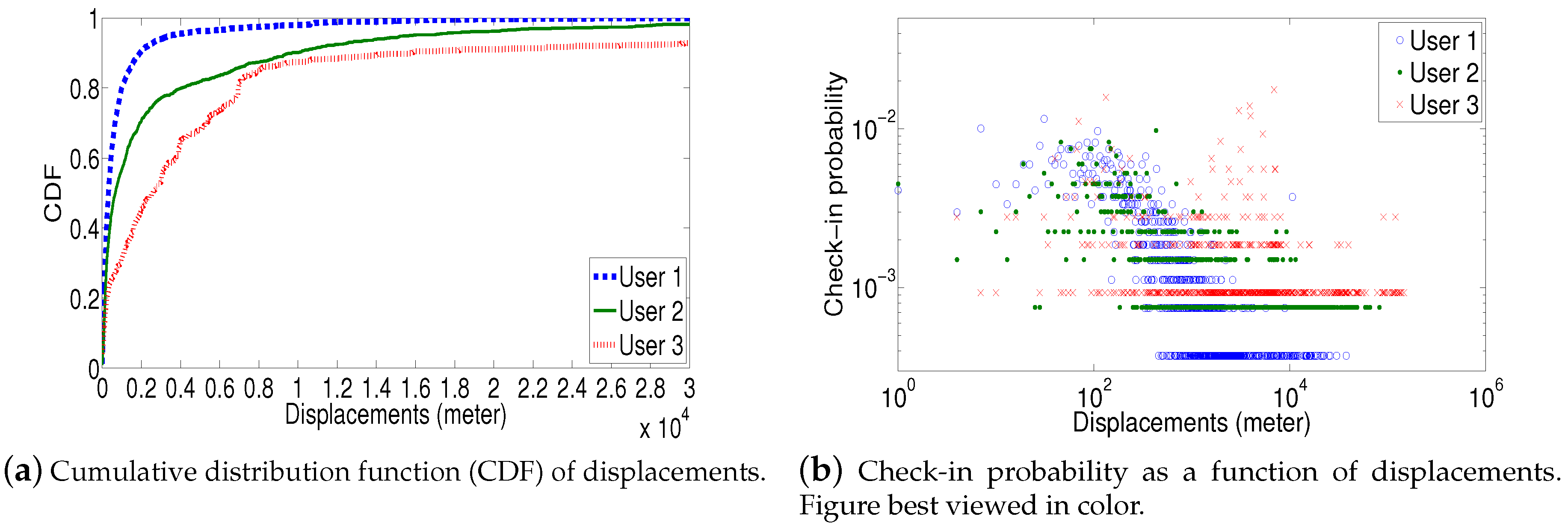
We randomly select three users who have over 1000 check-ins to demonstrate their heterogeneous mobility patterns. Figure 1a shows the cumulative distribution function (CDF) of users’ displacements between two consecutive check-ins (In our dataset, each location is associated with longitude and latitude, which can be used to calculate the distance between two locations.). We observe that user 1 mainly travels short distances, i.e., over 90% of her trips are less than 2 km. Only 2% of the user’s displacements are over 10 km. On the other hand, user 3 often travels farther: about 10% of her displacements are over 15 km and the longest displacement is 146.4 kilometers. User 2 behaves in the “averaged” way that user 1 and user 3 do. This result demonstrates the uniqueness of users’ displacement distribution.
In Figure 1b, we plot the check-in probability as a function of displacements. It is clear that user 1’s check-in behavior demonstrates the power-law like distribution (the user’s visited locations tend to be within short distances, while long travels happen with much lower probabilities), but the distribution for user 3, although also shows power-law property, it looks much more “scattered” (i.e., significantly deviating from user 1’s check-in behavior). This again proves that users’ displacement distributions are heterogeneous, thus are undesirable to be modeled in a universal way like in [12].
3.2. Temporal Influence
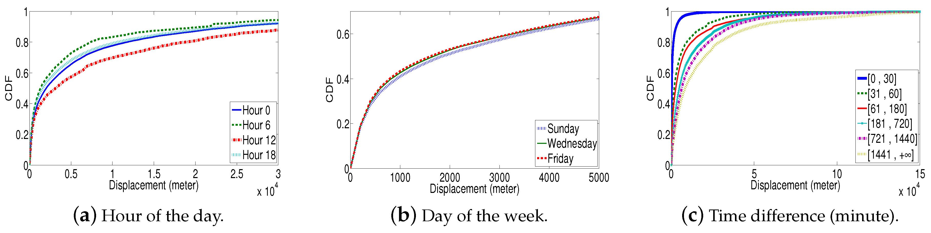
We investigated the temporal influence (Note that to demonstrate temporal influence, we use all users’ check-in data (Chicago).) from three aspects, i.e., hour of the day, day of the week and time difference between two consecutive check-ins. Figure 2a shows the CDF of displacements in four selected hours during a day. Obvious gaps can be observed among different hours: users tend to travel far during 12 h, probably due to trips to restaurants; on the other hand, most people have dinner at 7 or later, so the displacements at 6 h (i.e., just finished work) are relatively short.
We then plotted the CDF of displacements for three selected days of the week (see Figure 2b). The differences among displacement distributions in different days, although observable, are not significant. Nevertheless, we still considered this type of temporal information in our approach since: (1) the minor differences only demonstrate all users’ behavior but fail to reflect the influence of day of the week on individual users; (2) it can be combined with other temporal information to accurately model users’ check-in behavior patterns.
Finally, the CDF of displacements in different time difference intervals (in minute) is shown in Figure 2c. The time differences are classified into six intervals: [0,30], [31,60], [61,180], [181,720], [721,1440] and [1441,+∞]. Obviously, the larger the time difference, the longer the displacements are; therefore, the time difference between two consecutive check-ins can be a promising type of temporal information for check-in behavior modeling.
4. STS: Spatial–Temporal–Semantic Location Recommendation
In this section, we describe our STS framework. In an LBSN, we denote a set of users by and a set of locations by . For each user u, her historical check-in records (in chronological order) is denoted by , where is u’s ith check-in consisting of the location and the corresponding temporal information . Note that contains the descriptive information such as longitude, latitude and category of the location.
We identify four types of temporal information: (1) hour of the day (denoted by ); (2) day of the week (denoted by ); (3) time difference between two consecutive check-ins (denoted by ); (4) sequence of time stamps of a user’s past check-ins in chronological order (denoted by ). The influence of the first three types of temporal information is shown in Section 3.2. The fourth type of temporal information is used to encode the effect of “sequence”. That is, conventional location recommendation models studied users’ check-in behavior patterns from a pool of historical check-ins without taking into account the sequence of such check-ins. This may ignore some important properties such as users’ preference transition [36] (e.g., a user likes checking-in at her favorite restaurant after shopping in the city center and then enjoys a cup of coffee near her apartment), which is important for personalized location recommendation.
By comprehensively modeling the temporal influence from four aspects mentioned above, we predict a user’s displacement from her current checked-in location to the next checked-in location, which is presented in the next subsection.
4.1. Displacement Prediction
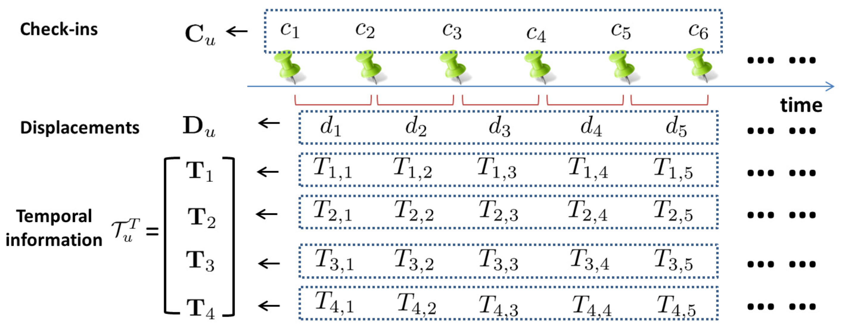
For a user u, we denote the vector of her displacements between two consecutive check-ins (in chronological order) by , which can be computed with the corresponding geographical location information (i.e., longitude and latitude information); the corresponding temporal information of the displacements is denoted by (i.e., 4-dimension temporal information corresponds to each displacement). Figure 3 illustrates the relationships among , and .
We treat as the independent variable, as the dependent variable and apply Gaussian process to predict users’ future displacements given the four types of temporal information. A Gaussian process [24] is a generalization of the Gaussian probability distribution, whereas a probability distribution describes random variables which are scalars or vectors (for multivariate distributions), a stochastic process governs the properties of functions. The distribution of a Gaussian process is fully characterized by its mean function and covariance function. A Gaussian process defines a distribution over functions, where f is a function that maps the input space to , i.e., . Let denotes an n-dimensional vector of function values at the corresponding n points . Formally, is a Gaussian process if for any finite subset , the marginal distribution over that finite subset follows a multivariate Gaussian distribution [24].
The purpose of our Gaussian process based model is to learn a latent function that maps user u’s temporal information to her displacement vector :
In order to take into account the noise, which is common in practice (e.g., GPS coordinates are not completely accurate), we assume an additive independent identically distributed Gaussian noise , with variance :
The joint distribution of the observed displacements and the function values to be predicted is obtained, according to the theory that the values of the function to be learned follow multivariate Gaussian distribution:
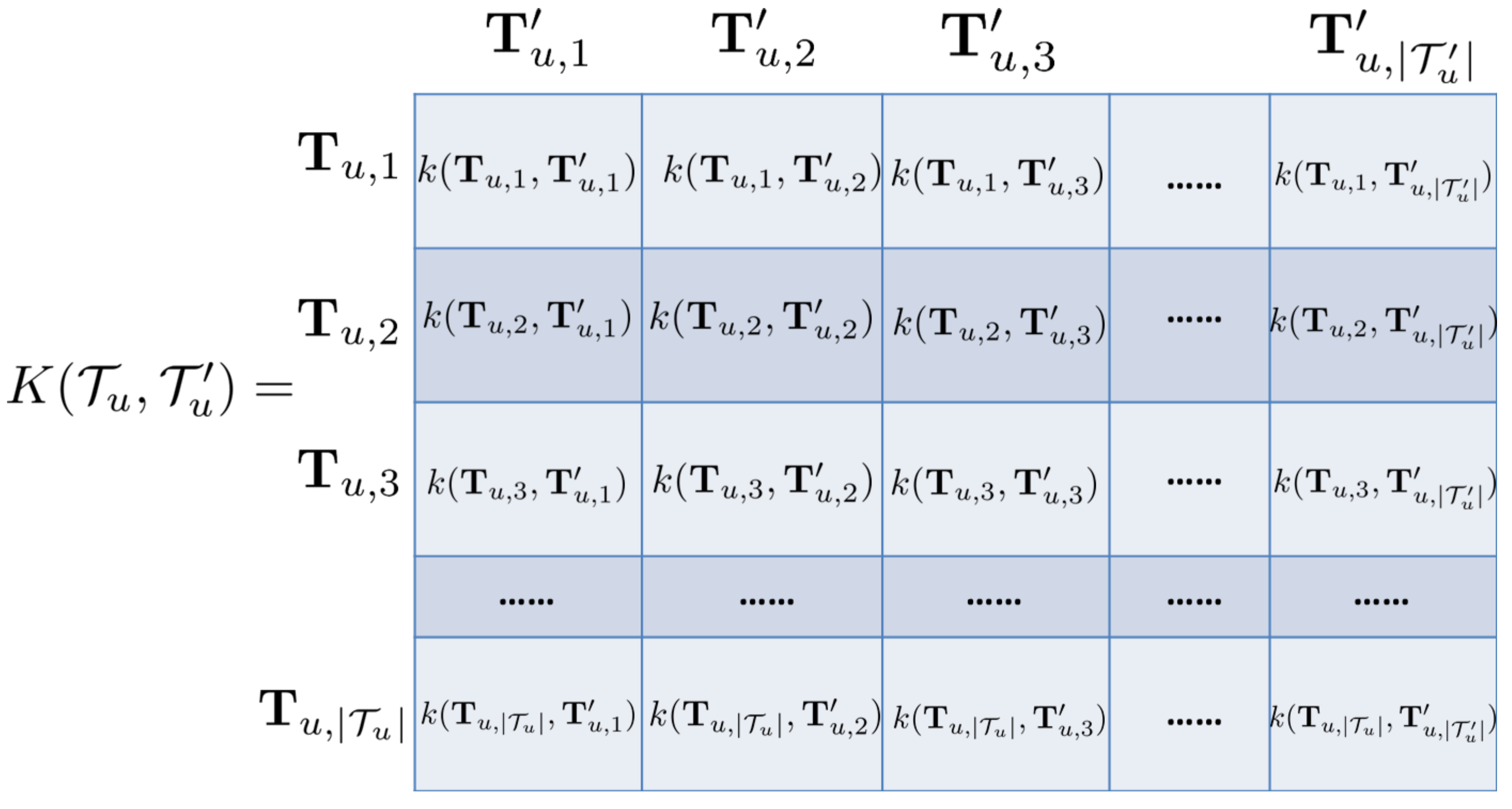
where I is identity matrix, is mean function and is covariance matrix. The th element of represents the covariance calculated at the rth and cth 4-dimension temporal information in . Accordingly, the elements of , and represent the covariances calculated at all 4-dimension temporal information pairs in (,), (, ) and , respectively. Figure 4 gives an example of covariance matrix .
By conditioning the joint Gaussian prior distribution on the observed temporal information, we derive the probability of :
We can obtain the estimated latent function , i.e., the predicted future displacements by the mean of its distribution:
Gaussian process also generates the variance of the distribution, which can be used to measure the confidence of the prediction:
From its definition, a Gaussian process regression model is fully specified by a mean function and a covariance function. In the following section, we discuss how to design these two functions for our displacement predictive model.
4.1.1. Mean Function and Covariance Function
For mean function, we use a simple form, which is the average of user u’s past displacements:
There are numerous covariance functions, making Gaussian process flexible in various application scenarios. We start with a well-known function called squared exponential covariance function for our model:
where and are 4-dimension temporal information associated with two displacements (indexed by m and n) of user u; h and are hyperparameters that control the scale (or variance) of the function output and the length-scale of the input, respectively. Since the four types of temporal information may have different impacts on users’ check-in activities, we combine them by assigning a weight to each type (i.e., , where ). We determine these weights by learning from the observed data. Note that although the four types of temporal information are combined to represent the temporal influence in a linear way, the interplay between temporal information of any pair of user u’s displacements is modeled non-linearly (i.e., in the form of a covariance matrix, see Figure 4), which is able to more accurately capture the temporal influence on users’ check-in behavior.
Note that we are not claiming that squared exponential covariance function is the most suitable function for displacement prediction. We leave as a future work a more detailed discussion on the tradeoff between the more sophisticated covariance functions (e.g., neural network covariance function) and the associated additional computational overheads.
4.1.2. Model Fitting
In this subsection, we discuss how to fit the model, including learning the covariance function hyperparameters and the weight of each type of temporal information.
According to the definition of Gaussian process, the distribution of observed data follows multivariate Gaussian distribution:
where are model parameters consisting of covariance function hyperparameters and temporal information weights. The corresponding negative log marginal likelihood is obtained:
Model fitting becomes a non-convex optimization problem of minimizing the negative log marginal likelihood L. We apply stochastic gradient descent (SGD) to learn model parameters , which are updated iteratively:
where is the learning rate. The optimization procedure completes if the predefined maximum number of iterations has reached or the negative log marginal likelihood at a certain iteration converges.
We find the derivatives of L with respect to the model parameters (covariance function hyperparameters h, , and the weight of each type of temporal information ):
where the derivative of covariance matrix with respect to each covariance hyperparameter is obtained (the matrix element is indexed by row m and column n):
and
The derivative of covariance matrix with respect to the weight of each type of temporal information is obtained (the matrix element is indexed by row m and column n):
4.2. Semantic-Aware Enhancement
Displacement prediction provides the estimation of users’ geographical movement for location recommendation. In this section, we propose a semantic-aware enhancement by studying the category information of users’ checked-in locations (Note that each location is associated with category information. For instance, a seafood restaurant belongs to the category of “food”.) to infer their time-aware preference distribution for recommendation.
We denote the category set in the system by . The purpose of the semantic-aware enhancement is to infer a user’s probability distribution of category information, i.e., the probability that the user will check-in at a location under a certain category given the temporal information constraints: . Note that we only consider two types of temporal information, i.e., hour of the day and day of the week when deriving category distribution.
For user u, the category distribution is estimated by counting the occurrence of a certain category in the given temporal context from her historical check-ins:
where is the number of occurrences of category given the temporal information , and is the number of user u’s check-ins. Note that the derived category probability distribution is subject to the condition that = 1. Based on such a category distribution, we are able to infer a user’s preference at a specified time frame and hence improve the accuracy of location recommendation.
4.3. A Unified Recommendation Framework
In this section, we develop a unified recommendation framework called STS to integrate displacement prediction and the semantic-aware enhancement to provide personalized top-N location recommendation for user u.
Given the temporal information , we denote user u’s predicted next displacement by (see Section 4.1). For a candidate location , we calculate the distance between user u’s current location and , denoted by . We then obtain the difference between and :
Theoretically, the smaller the difference , the more likely that the location will be checked-in. Based on such a geographical distance difference, we derive the probability that the candidate location will be checked-in by user u.
where n is a design parameter that constrains the error of displacement prediction. A suitable n produces a reasonable (An extremely small n cannot constrain the error of displacement prediction (e.g., when n = 1, prediction errors of 10 m and 100 m produce check-in probabilities of 0.1 and 0.01 respectively, which are not reasonably comparable in the real world); and an extremely large n makes approach to 1, which actually eliminates the geographical influence.) check-in probability that is combined with semantic-aware check-in probability for recommendation. The choice of n depends on the dataset used, we will give an example for a real LBSN in Section 5.
In the following, present the semantic influence on the check-in probability. We denote the category of the candidate location by . Based on user u’s category distribution (see Section 4.2), we obtain the probability that user u will check-in at some location under category :
Finally, we fuse the spatial–temporal influence and semantic–temporal influence to derive the final probability that user u will check-in at the candidate location :
Note that we also tried other fusion methods like weighted sum of and ; however, the experimental results show that the product rule always outperforms the sum rule. This is also consistent with the observations in [5]. So in this work, we only use the product rule as the fusion method.
In this way, we derive user u’s check-in probability for all candidate locations; the top-N locations that have the highest check-in probabilities are recommended.
5. Evaluation and Discussion
5.1. Experimental Settings
5.1.1. Datasets
In order to evaluate the proposed personalized STS framework, we used real check-in datasets collected from Gowalla. We used the Gowalla APIs to collect users’ check-in data (longitude, latitude, time stamps, etc.) generated before 1 June 2011 in the following cities: Austin, Chicago, Houston, Los Angeles and San Francisco [36]. The statistics of the check-in data in different cities are summarized in Table 1, in which denotes the number of users, denotes the number of locations, denotes the number of check-ins, denotes the average number of visited users for a location and was used to denote the average number of visited locations for a user.
We also collected the category information of each observed location. The locations in Gowalla were grouped into 7 main categories, i.e., Community, Entertainment, Food, Nightlife, Outdoors, Shopping and Travel. In each main category, the locations were classified into different subcategories (there are totally 134 categories at the second level). Note that certain subcategories may be further divided into more specific categories but due to data incompleteness, we only considered the first and second category levels in our experiments.
For each user, we sorted her historical check-ins in chronological order. The first of check-ins were selected as training data to learn a location recommendation model and the remaining ones were used for testing.
5.1.2. Baselines
We compared our STS framework to the state-of-the-art location recommendation methods. BaseMF [42]: this model only considers users’ preference on locations for recommendation without taking into account other side information (e.g., spatial–temporal influence). SGD was applied to fit the model by learning over user-location matrix. The Top-N recommendation was produced by sorting the candidate locations in descending order of the predicted preferences. GeoCF [12]: the geographical influence was captured using the power-law distribution, which is integrated with a user-based collaborative filtering algorithm. A unified POI recommendation framework is proposed to linearly combine the user preference and geographical influence. PTMF [36]: this approach consists of two stages where at the first stage, users’ preference transitions (represented by categories of the checked-in locations) was predicted by a BaseMF model, and at the second stage, users’ preferences on locations in the corresponding categories (predicted by the first stage) were inferred by another BaseMF model. The Top-N recommendation was provided based on the category-aware preference prediction. iGSLR [5]: similar to our STS framework, this approach builds a personalized recommendation model for individual users by applying a kernel density estimation method to model the geographical influence. A unified recommendation framework was used to combine users’ preference (derived by user-based collaborative filtering) and geographical influence for final recommendation. TempMF [1]: this model studies the temporal influence from the aspects of non-uniformness and consecutiveness (see Section 2 for more details). Matrix factorization is used to integrate the temporal influence in a linear way (i.e., linearly aggregating users’ preferences in different hours). Distance2Pre [43]: this model focuses on modeling the correlation between user and distance. Users’ sequential preferences are firstly learned by modeling check-in sequences. Then, users’ spatial preference are learned by modeling distances between the successively visited POIs. A non-linear fusion method is proposed to merge the two types of preferences for recommendation. POI2Vec [44]: this method predicts the potential visitors for a given POI in the near future. A binary tree is used to cluster the nearby POIs into the same region, and a POI is assigned to multiple regions to strengthen its spatial influence. Then, a method that jointly models POI sequential transition and user preference was developed.
For matrix factorization based models that initialize latent factors based on certain distribution (e.g., uniform distribution in the range of [0,1]), 5-folder cross-validation was conducted and the averaged results were reported.
5.1.3. Metrics
The goal of a location recommendation model is, given a user’s current check-in information, to recommend her top-N highest ranked locations such that her next check-in will follow one of the recommended locations. To measure the accuracy of a location recommendation method, we used Precision@N, which is the ratio of the successfully predicted locations to the top-N recommendations:
where denotes users set of the testing dataset, N denotes the size of the recommendation list, denotes the the top-N recommendation list provided for user u by the recommendation model and denotes the true location list checked in by user u. This metric can be used to indicate the hit ratio of the top-N recommendation.
Meanwhile, we also use mean reciprocal rank (MRR), a popular ranking metric to measure recommendation quality by finding out how far from the top of the list the first successfully predicted location is (averaged over all test cases):
where is the position of the first successfully predicted location in the recommendation list returned for the ith user.
5.2. Experimental Results
In this section, we first validate the design of the proposed STS framework from three aspects, i.e., the effect of data sparsity, the effect of different types of temporal information and the effect of category information. The covariance function parameters h, and are set to 1, 1 and 50 respectively; the learning rate of SGD is set to 0.00001; the weights of the four types of temporal information are initialized as 1; the n that constrains the displacement prediction error (see Equation (19)) is set to 6 for Chicago and Houston data, 8 for Austin and San Francisco data and 10 for Los Angeles data. We then compare the performance of STS with that of the state-of-the-art location recommendation models.
5.2.1. Effect of Data Sparsity
Table 2 summarizes the performance of STS framework with different volumes of training data (i.e., first x% of each user’s check-ins). It is clear that for all datasets, both precision and MRR increase with the increasing volume of training data; however, in LBSNs, users’ check-in information is typically sparse, which influences the performance of recommendation models. To validate STS in a sparsity setting, we set x to as low as 25, and observe that STS still provides reasonably high recommendation quality compared to other location recommendations models that work under the condition that 70% of users’ check-ins are used for model training (see comparison studies presented in Section 5.2.4).
In the following experiments, we set x to 70 by default to split training data and test data for all location recommendation models.
5.2.2. Effect of Temporal Information
Figure 5 shows, across five cities, the performance comparison among four STS variants, which only consider one of the four types of temporal information individually (i.e., hour of the day, day of the week, time difference between two consecutive check-ins and time stamps) and the full STS framework that relies on all temporal information. That is, for a STS variant, in Figure 3 is a one dimension vector.
We observe that any individual temporal information is not sufficient to model users’ check-in behavior but when these types of temporal information are combined, the accuracy of users’ displacement prediction is evidently improved. Figure 5a,b also show the importance of various types of temporal information. There are no observations indicating which type of temporal information is consistently more important than others in displacement prediction, demonstrating the complexity and heterogeneity of the datasets. Nevertheless, with respect to Chicago data, we observe that day of the week is less important than hour of the day and time difference. This is consistent with the data analysis results presented in Section 3 (see Figure 2). We also notice that time stamps outperforms other types of temporal information in some scenarios (e.g., San Francisco data and Los Angeles data), demonstrating the importance of considering the sequence of users’ check-in behavior for mobility modeling.
5.2.3. Effect of Category Information
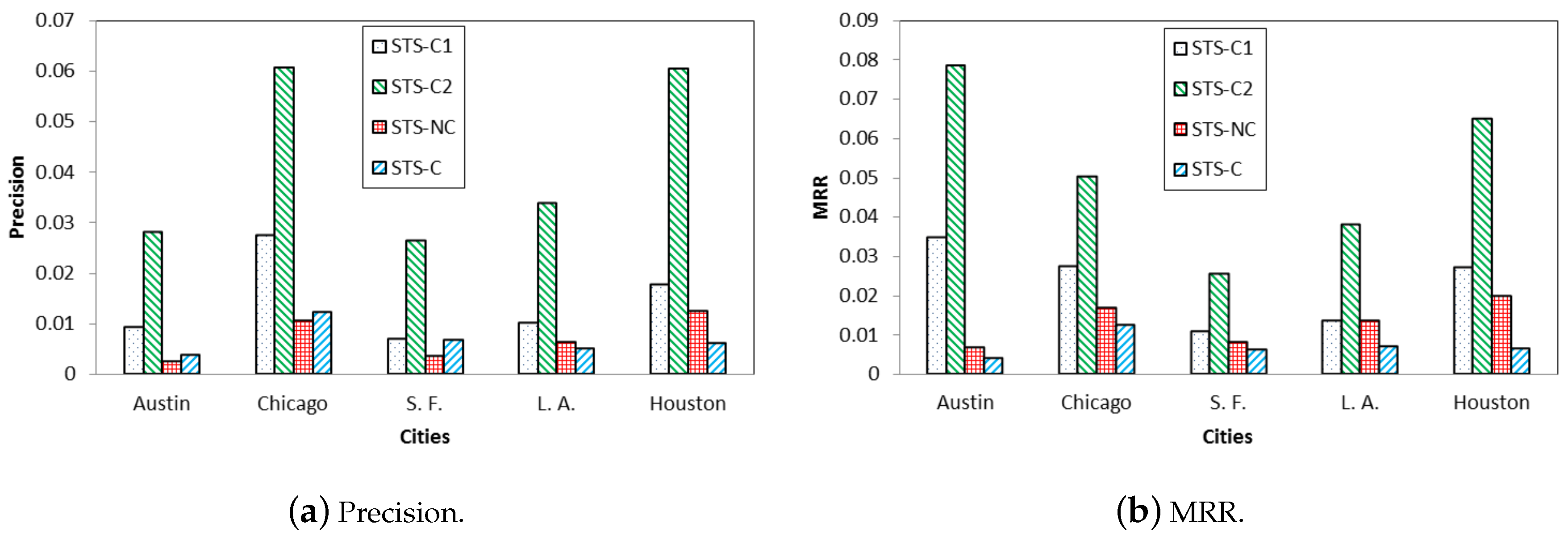
We finally study the impact of the category information. Figure 6 shows the comparison among four STS variants: (1) the one that applies category level 1 to model semantic influence, named STS-C1; (2) the one that applies category level 2, named STS-C2; (3) the one that does not consider any semantic influence, named STS-NC (e.g., only displacement prediction is used to make recommendation, see Equation (19); (4) the one that only relies on semantic influence without taking into account any geographical influence, named STS-C (see Equation (20)).
We observe that when category level 2 is applied, STS-C2 significantly outperforms STS-C1 that relies on category level 1. This result demonstrates the importance of category level selection. In comparison studies presented in the next subsection, STS framework uses category level 2 by default. When no category information is considered (i.e., only displacement prediction is used for recommendation), STS-NC’s performance is not promising. This is due to the common clustering phenomenon of locations, i.e., a collection of locations are clustered where distances among the locations are short (e.g., many restaurants and shops are located in a shopping mall). So even if the displacement prediction error is as low as 100 m, it is still challenging to successfully predict the target locations in the presence of location clustering phenomenon. On the other hand, if only category information is used, the performance of STS-C is not promising either, indicating the effectiveness of jointly modeling geographical influence and semantic influence (considering temporal influence).
One may notice that the performance of STS-NC (i.e., only GP based displacement prediction is used for recommendation) is lower than that of the state-of-the-art methods (see Table 3), thus questioning the effectiveness of our GP based approach in location recommendation. However, we argue that the state-of-the-art methods are mostly hybrid models that combine the geographical influence with many other factors like collaborative filtering to make recommendation so it is unfair to compare the our GP based displacement prediction with these models directly. Actually, when only geographical influence is considered, our GP based method improves the performance of variants of GeoCF and iGSLR (GeoCF and iGSLR are two location recommendation models that explore geographical influence.) (i.e., only the components that capture the geographical influence are used) by 15.24% and 12.41% respectively in terms of precision. We next elaborate on the comparison studies between our approach and the state-of-the-art models.
5.2.4. Comparison Studies
We compare the performance of STS framework and that of the state-of-the-art location recommendation methods (see Section 5.1.2). By cross-validation of the BaseMF, we set latent factor vector dimensionality, learning rate and regularization parameter to 10, 0.0001 and 0.01, respectively; for PTMF, category level 2 is considered, where the latent factor vector dimensionality, learning rate and regularization parameters are set to 5, 0.0001 and 0.01, respectively; for TempMF, we set latent factor vector dimensionality, learning rate, user-preference parameter, location-characteristic parameter and time regularization parameter to 10, 0.0001, 2, 2 and 1, respectively; for POI2Vec, the number of dimensions, region size threshold and learning rate are set at 200, 0.1, 0.005, respectively; for Distance2Pre, the learning rate, regularization parameter and the number of dimensions are set at 0.01, 0.001 and 20, respectively.
Table 3 summarizes the comparison results using the five datasets when top-10 recommendation is provided. As expected, BaseMF performs worst since it does not consider various factors such as temporal and geographical influence, which significantly impact location prediction. GeoCF, by modeling geographical influence using power-law distribution, evidently improves BaseMF in terms of both precision and MRR. For GeoCF, the social influence weighting parameter, geographical influence weighting parameter and tuning parameter are set to 0.1, 0.1 and 0.05, respectively. iGSLR, on the contrary, models geographical influence for individual users by applying a kernel density estimation approach. For iGSLR, like the settings of the original article, the kernel function is set as a normal kernel and the bandwidth is set as ( denotes the standard deviation of the distance samples, denotes the number of distance samples, and they can be obtained from the corresponding sample data). Such a personalized method outperforms GeoCF that models geographical influence in a universal way. On the other hand, TempMF focuses on temporal influence on users’ check-in behavior. Experiments results show that TempMF generally outperforms iGSLR in terms of precision (except for Los Angeles data) but is slightly outperformed by iGSLR in terms of MRR (except for San Francisco data). By modeling the mutual influence between regions and POIs, as well as capturing POI sequential transition, POI2Vec further improves TempMF. PTMF outperforms other matrix factorization based models and POI2Vec, proving the importance of semantic influence and also demonstrating that learning users’ preference transition evidently boosts recommendation performance. Distance2Pre, although only considers geographical influence, outperforms PTMF. This is because Distance2Pre applies more advanced Gated Recurrent Unit (GRU) to model users’ sequential check-in behavior, demonstrating the advantage of non-linear modeling methods. In all cases, STS outperforms other recommendation models by: (1) non-linearly combining various types of temporal information for temporal-aware mobility prediction; (2) modeling temporal-aware semantic influence to infer users’ preferences; (3) building recommendation models for individual users for personalization.
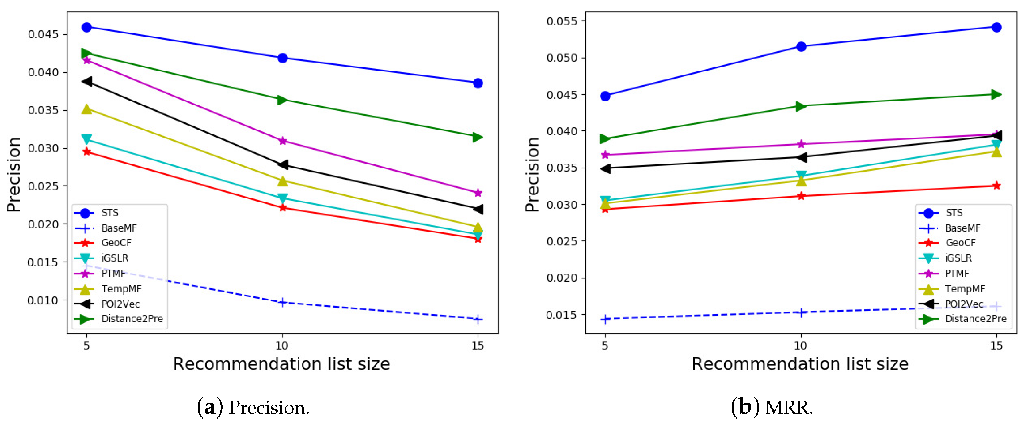
Finally, Figure 7 shows the precision and MRR (averaged over three datasets) of different recommendation models with different recommendation list sizes. Similar to previous experimental results, all models outperform the baseline BaseMF. TempMF produces higher precision but slightly lower MRR than iGSLR does, demonstrating that although the hit ratio is higher, TempMF’s successfully predicted locations are at the relatively lower positions of the returned recommendation lists. PTMF outperforms TempMF, iGSLR, GeoCF and POI2Vec, but is beaten by the deep learning model Distance2Pre. Finally, by sophisticated modeling and incorporating various influence factors, STS outperforms all other baselines in all settings. In summary, by averaging results when different datasets and recommendation list sizes are applied, STS improves GeoCF, iGSLR TempMF, POI2Vec, PTMF and Distance2Pre by 81.90%, 72.95%, 57.46%, 46.53%, 32.29% and 23.25% in terms of precision and 61.93%, 47.21%, 49.85%, 40.27%, 31.76% and 18.69% in terms of MRR.
5.3. Discussion
The time complexity of STS is mainly determined by the inversion of a matrix (i.e., Gaussian process based displacement prediction. See Equation (5)). The standard methods require the time for a matrix. Such a computation procedure can be improved by applying faster matrix multiplication method such as Coppersmith–Winograd algorithm [45]. Alternatively, approximation techniques like variational Bayesian inference [46] can be applied to accelerate the learning process. Since STS framework is built for individual users for personalization, it can be completely and efficiently parallelized (compared to collaborative filtering based approaches that learn over all users’ data) to cater to large-scale datasets.
Although social networking is an important feature of a location based social network, quite a few previous studies have demonstrated that the influence of social information exists, but its effect on users’ check-in behavior is quite limited [10,14,36], so in this work, we do not consider social influence to reduce the complexity of the STS framework.
Similar to other location recommendation models, the extent of data sparsity influences the performance of STS. Theoretically, STS works even if the target user has only a couple of check-ins. Moreover, Gaussian process provides the variance of the displacement prediction, which can be used to indicate the confidence of the prediction. We have demonstrated in the above evaluation section how the performance of STS varies with different size of training data.
With the promotion of more and more recommendation service platforms of mobile terminals, our location recommendation algorithm will provide strong support for many recommendation services involving location information (such as hotel recommendation, scenic spot recommendation, shopping venue recommendation, entertainment venue recommendation, etc.), so as to effectively improve the user’s experience satisfaction.
6. Conclusions
In this work, we presented a personalized location recommendation framework called STS. A Gaussian process is applied to systematically and non-linearly integrate various types of temporal and spatial information to predict each user’s temporal-aware displacement. A stochastic gradient descent based optimization procedure is developed to fit the model. Moreover, we take into account the category information of each user’s checked-in locations to infer the probability that the user will check-in at specific categories given the temporal context. A unified recommendation framework is proposed to combine displacement prediction and category probability distribution inference to provide the final top-N location recommendation. Extensive experiments demonstrate that our algorithm significantly outperforms the state-of-the-art models in terms of precision and MRR.
Several research directions will be pursued in a future work: (1) exploring more sophisticated covariance functions to better model temporal influence and geographic influence; (2) adopting ranking techniques, e.g., learning to rank to improve recommendation ranking performance; (3) investigating more textual information (e.g., tips, reviews from users’ check-ins record) by applying advanced NLP models like transformers to enhance semantic influence modeling and mine various user activities information; (4) introducing some new displacement calculation methods to compensate for the low positioning accuracy.
Author Contributions
Conceptualization, methodology, software, data curation and writing, Xin Liu and Wenchao Li; conceptualization and methodology, Jiyong Zhang, Guiguang Ding and Yaoqi Sun; funding acquisition, Chenggang Yan. All authors have read and agreed to the published version of the manuscript.
Funding
This research is supported by National Nature Science Foundation of China (61931008, 61671196, 61701149, 61801157, 61971268, 61901145, 61901150, 61972123), the National Natural Science Major Foundation of Research Instrumentation of PR China under Grants 61427808, Zhejiang Province Nature Science Foundation of China (LR17F030006,Q19F010030), 111 Project, No. D17019.
Conflicts of Interest
The authors declare no conflict of interest.
References
- Gao, H.; Tang, J.; Hu, X.; Liu, H. Exploring temporal effects for location recommendation on location-based social networks. In Proceedings of the 7th ACM Conference on Recommender Systems, Hong Kong, China, 12–16 October 2013; pp. 93–100. [Google Scholar]
- Liu, X.; Liu, Y.; Li, X. Exploring the Context of Locations for Personalized Location Recommendations. In Proceedings of the 25th International Joint Conference on Artificial Intelligence, New York, NY, USA, 9–15 July 2016; pp. 1188–1194. [Google Scholar]
- Gao, R.; Li, J.; Li, X.; Song, C.; Chang, J.; Liu, D.; Wang, C. STSCR: Exploring spatial-temporal sequential influence and social information for location recommendation. Neurocomputing 2018, 319, 118–133. [Google Scholar] [CrossRef]
- Liu, J.; Zhang, Z.; Liu, C.; Qiu, A.; Zhang, F. Exploiting Two-Dimensional Geographical and Synthetic Social Influences for Location Recommendation. ISPRS Int. J. Geo-Inf. 2020, 9, 285. [Google Scholar] [CrossRef]
- Zhang, J.D.; Chow, C.Y. iGSLR: Personalized geo-social location recommendation: A kernel density estimation approach. In Proceedings of the 21st ACM SIGSPATIAL International Conference on Advances in Geographic Information Systems, Orlando, FL, USA, 5–8 November 2013; pp. 334–343. [Google Scholar]
- Yang, D.; Zhang, D.; Yu, Z.; Wang, Z. A sentiment-enhanced personalized location recommendation system. In Proceedings of the 24th ACM Conference on Hypertext and Social Media, Paris, France, 1–3 May 2013; pp. 119–128. [Google Scholar]
- Kurashima, T.; Iwata, T.; Hoshide, T.; Takaya, N.; Fujimura, K. Geo topic model: Joint modeling of user’s activity area and interests for location recommendation. In Proceedings of the 6th ACM International Conference on Web Search and Data Mining, Rome, Italy, 4–8 February 2013; pp. 375–384. [Google Scholar]
- Khazaei, E.; Alimohammadi, A. Context-Aware Group-Oriented Location Recommendation in Location-Based Social Networks. ISPRS Int. J. Geo-Inf. 2019, 8, 406. [Google Scholar] [CrossRef] [Green Version]
- Lu, Z.; Wang, H.; Mamoulis, N.; Tu, W.; Cheung, D.W. Personalized location recommendation by aggregating multiple recommenders in diversity. GeoInformatica 2017, 21, 459–484. [Google Scholar] [CrossRef]
- Cho, E.; Myers, S.A.; Leskovec, J. Friendship and mobility: User movement in location-based social networks. In Proceedings of the 17th ACM SIGKDD International Conference on Knowledge Discovery and Data Mining, San Diego, CA, USA, 21–24 August 2011; pp. 1082–1090. [Google Scholar]
- Lian, D.; Zhao, C.; Xie, X.; Sun, G.; Chen, E.; Rui, Y. GeoMF: Joint geographical modeling and matrix factorization for point-of-interest recommendation. In Proceedings of the 20th ACM SIGKDD International Conference on Knowledge Discovery and Data Mining, New York, NY, USA, 24–27 August 2014; pp. 831–840. [Google Scholar]
- Ye, M.; Yin, P.; Lee, W.C.; Lee, D.L. Exploiting Geographical Influence for Collaborative Point-of-interest Recommendation. In Proceedings of the 34th International ACM SIGIR Conference on Research and Development in Information Retrieval, Beijing, China, 25–29 July 2011; pp. 325–334. [Google Scholar]
- Noulas, A.; Scellato, S.; Lathia, N.; Mascolo, C. Mining user mobility features for next place prediction in location-based services. In Proceedings of the 12th IEEE International Conference on Data Mining, Brussels, Belgium, 10–13 December 2012; pp. 1038–1043. [Google Scholar]
- Cheng, C.; Yang, H.; King, I.; Lyu, M.R. Fused matrix factorization with geographical and social influence in location-based social networks. In Proceedings of the 26th AAAI Conference on Artificial Intelligence, Toronto, ON, Canada, 22–26 July 2012; pp. 17–23. [Google Scholar]
- Yuan, Q.; Cong, G.; Ma, Z.; Sun, A.; Thalmann, N.M. Time-aware point-of-interest recommendation. In Proceedings of the 36th International ACM SIGIR Conference on Research and Development in Information Retrieval, Dublin, Ireland, 28 July–1 August 2013; pp. 363–372. [Google Scholar]
- Yan, C.; Tu, Y.; Wang, X.; Zhang, Y.; Hao, X.; Zhang, Y.; Dai, Q. STAT: Spatial-temporal attention mechanism for video captioning. IEEE Trans. Multimed. 2019, 22, 229–241. [Google Scholar] [CrossRef]
- Hu, B.; Ester, M. Spatial topic modeling in online social media for location recommendation. In Proceedings of the 7th ACM Conference on Recommender Systems, Hong Kong, China, 12–16 October 2013; pp. 25–32. [Google Scholar]
- Liu, B.; Fu, Y.; Yao, Z.; Xiong, H. Learning geographical preferences for point-of-interest recommendation. In Proceedings of the 19th ACM SIGKDD International Conference on Knowledge Discovery and Data Mining, Chicago, IL, USA, 11–14 August 2013; pp. 1043–1051. [Google Scholar]
- Zhao, S.; Zhao, T.; King, I.; Lyu, M.R. Geo-teaser: Geo-temporal sequential embedding rank for point-of-interest recommendation. In Proceedings of the 26th International Conference on World Wide Web Companion, Perth, Australia, 3–7 April 2017; pp. 153–162. [Google Scholar]
- Liu, T.; Liao, J.; Wu, Z.; Wang, Y.; Wang, J. Exploiting geographical-temporal awareness attention for next point-of-interest recommendation. Neurocomputing 2020, 400, 227–237. [Google Scholar] [CrossRef]
- Wang, H.; Shen, H.; Ouyang, W.; Cheng, X. Exploiting POI-Specific Geographical Influence for Point-of-Interest Recommendation. In Proceedings of the 27th International Joint Conference on Artificial Intelligence, Stockholm, Sweden, 13–19 July 2018; pp. 3877–3883. [Google Scholar]
- Cai, L.; Xu, J.; Liu, J.; Pei, T. Integrating spatial and temporal contexts into a factorization model for POI recommendation. Int. J. Geogr. Inf. Sci. 2018, 32, 524–546. [Google Scholar]
- Li, H.; Hong, R.; Wu, Z.; Ge, Y. A spatial-temporal probabilistic matrix factorization model for point-of-interest recommendation. In Proceedings of the 2016 SIAM International Conference on data Mining, Miami, FL, USA, 5–7 May 2016; pp. 117–125. [Google Scholar]
- Rasmussen, C.E.; Williams, C.K.I. Gaussian Processes for Machine Learning; The MIT Press: Cambridge, MA, USA, 2005. [Google Scholar]
- Clauset, A.; Shalizi, C.R.; Newman, M.E. Power-law distributions in empirical data. SIAM Rev. 2009, 51, 661–703. [Google Scholar] [CrossRef] [Green Version]
- Li, X.; Cong, G.; Li, X.L.; Pham, T.A.N.; Krishnaswamy, S. Rank-geofm: A ranking based geographical factorization method for point of interest recommendation. In Proceedings of the 38th International ACM SIGIR Conference on Research and Development in Information Retrieval, Santiago, Chile, 9–13 August 2015; pp. 433–442. [Google Scholar]
- Ma, C.; Zhang, Y.; Wang, Q.; Liu, X. Point-of-interest recommendation: Exploiting self-attentive autoencoders with neighbor-aware influence. In Proceedings of the 27th ACM International Conference on Information and Knowledge Management, Torino, Italy, 22–26 October 2018; pp. 697–706. [Google Scholar]
- Ying, H.; Chen, L.; Xiong, Y.; Wu, J. PGRank: Personalized geographical ranking for point-of-interest recommendation. In Proceedings of the 25th International Conference Companion on World Wide Web, Montreal, QC, Canada, 11–15 April 2016; pp. 137–138. [Google Scholar]
- Liu, C.; Liu, J.; Xu, S.; Wang, J.; Liu, C.; Chen, T.; Jiang, T. A Spatiotemporal Dilated Convolutional Generative Network for Point-Of-Interest Recommendation. ISPRS Int. J. Geo-Inf. 2020, 9, 113. [Google Scholar] [CrossRef] [Green Version]
- Ying, Y.; Chen, L.; Chen, G. A temporal-aware POI recommendation system using context-aware tensor decomposition and weighted HITS. Neurocomputing 2017, 242, 195–205. [Google Scholar] [CrossRef]
- Aliannejadi, M.; Rafailidis, D.; Crestani, F. A joint two-phase time-sensitive regularized collaborative ranking model for point of interest recommendation. IEEE Trans. Knowl. Data Eng. 2019, 32, 1050–1063. [Google Scholar] [CrossRef] [Green Version]
- Yao, Z. Exploiting human mobility patterns for point-of-interest recommendation. In Proceedings of the 11th ACM International Conference on Web Search and Data Mining, Marina Del Rey, CA, USA, 5–9 February 2018; pp. 757–758. [Google Scholar]
- Chang, B.; Park, Y.; Park, D.; Kim, S.; Kang, J. Content-Aware Hierarchical Point-of-Interest Embedding Model for Successive POI Recommendation. In Proceedings of the 27th International Joint Conference on Artificial Intelligence, Stockholm, Sweden, 13–19 July 2018; pp. 3301–3307. [Google Scholar]
- Liu, B.; Xiong, H. Point-of-interest recommendation in location based social networks with topic and location awareness. In Proceedings of the 13th SIAM International Conference on Data Mining, Austin, TX, USA, 2–4 May 2013; pp. 396–404. [Google Scholar]
- Yin, Z.; Cao, L.; Han, J.; Zhai, C.; Huang, T. Geographical topic discovery and comparison. In Proceedings of the 20th International Conference on World Wide Web, Hyderabad, India, 28 March–1 April 2011; pp. 247–256. [Google Scholar]
- Liu, X.; Liu, Y.; Aberer, K.; Miao, C. Personalized Point-of-interest Recommendation by Mining Users’ Preference Transition. In Proceedings of the 22nd ACM International Conference on Information & Knowledge Management, San Francisco, CA, USA, 27 October–10 November 2013; pp. 733–738. [Google Scholar]
- Hao, P.Y.; Cheang, W.H.; Chiang, J.H. Real-time event embedding for POI recommendation. Neurocomputing 2019, 349, 1–11. [Google Scholar] [CrossRef]
- Lian, D.; Ge, Y.; Zhang, F.; Yuan, N.J.; Xie, X.; Zhou, T.; Rui, Y. Scalable content-aware collaborative filtering for location recommendation. IEEE Trans. Knowl. Data Eng. 2018, 30, 1122–1135. [Google Scholar] [CrossRef]
- Zhang, J.D.; Chow, C.Y.; Zheng, Y. ORec: An opinion-based point-of-interest recommendation framework. In Proceedings of the 24th ACM International on Conference on Information and Knowledge Management, Melbourne, Australia, 19–23 October 2015; pp. 1641–1650. [Google Scholar]
- Zhou, X.; Mascolo, C.; Zhao, Z. Topic-enhanced memory networks for personalised point-of-interest recommendation. In Proceedings of the 25th ACM SIGKDD International Conference on Knowledge Discovery & Data Mining, Anchorage, AK, USA, 4–8 August 2019; pp. 3018–3028. [Google Scholar]
- Yin, H.; Wang, W.; Wang, H.; Chen, L.; Zhou, X. Spatial-aware hierarchical collaborative deep learning for POI recommendation. IEEE Trans. Knowl. Data Eng. 2017, 29, 2537–2551. [Google Scholar] [CrossRef]
- Mnih, A.; Salakhutdinov, R.R. Probabilistic matrix factorization. In Proceedings of the 21st International Conference on Neural Information Processing Systems, Vancouver, BC, Canada, 8–11 December 2008; pp. 1257–1264. [Google Scholar]
- Cui, Q.; Tang, Y.; Wu, S.; Wang, L. Distance2Pre: Personalized Spatial Preference for Next Point-of-Interest Prediction. In Proceedings of the 23rd Pacific-Asia Conference on Knowledge Discovery and Data Mining, Macau, China, 14–17 April 2019; pp. 289–301. [Google Scholar]
- Feng, S.; Cong, G.; An, B.; Chee, Y.M. Poi2vec: Geographical latent representation for predicting future visitors. In Proceedings of the 31st t AAAI Conference on Artificial Intelligence, San Francisco, CA, USA, 4–10 February 2017; pp. 102–108. [Google Scholar]
- Coppersmith, D.; Winograd, S. Matrix multiplication via arithmetic progressions. In Proceedings of the 19th Annual ACM Symposium on Theory of Computing, New York, NY, USA, 25–27 May 1987; pp. 1–6. [Google Scholar]
- Fox, C.W.; Roberts, S.J. A tutorial on variational Bayesian inference. Artif. Intell. Rev. 2012, 38, 85–95. [Google Scholar] [CrossRef]
Figure 1.
Heterogeneous mobility behaviors.

Figure 2.
Temporal influence.

Figure 3.
An example of user u’s check-in records , vector of displacements and the corresponding 4-dimension temporal information .
Figure 3.
An example of user u’s check-in records , vector of displacements and the corresponding 4-dimension temporal information .

Figure 4.
An example of user u’s covariance matrix , where is the covariance function that calculates the covariance of the given pair of temporal information vectors. denotes the cardinality of a set.
Figure 4.
An example of user u’s covariance matrix , where is the covariance function that calculates the covariance of the given pair of temporal information vectors. denotes the cardinality of a set.

Figure 5.
Temporal influence.

Figure 6.
Impact of semantic influence.

Figure 7.
Performance comparison with varying recommendation list size.


Table 1.
The statistics of experimental data.
| Austin | 24,070 | 51,118 | 1,935,677 | 21.95 | 46.62 |
| Chicago | 13,845 | 37,050 | 486,558 | 7.53 | 20.16 |
| Houston | 11,138 | 29,383 | 512,977 | 9.89 | 26.08 |
| L.A. | 21,633 | 75,301 | 1,296,953 | 10.06 | 35.02 |
| S.F. | 21,585 | 64,758 | 1,542,133 | 13.76 | 41.29 |
Table 2.
Influence of the volume of training data (top-10 recommendation).
| x% For Training | Houston | Chicago | Los Angeles | San Francisco | Austin | |||||
|---|---|---|---|---|---|---|---|---|---|---|
| Precision | MRR | Precision | MRR | Precision | MRR | Precision | MRR | Precision | MRR | |
| 25% | 0.0421 | 0.0452 | 0.0456 | 0.0362 | 0.0241 | 0.0285 | 0.0172 | 0.0168 | 0.0220 | 0.0625 |
| 50% | 0.0522 | 0.0567 | 0.0502 | 0.0421 | 0.0299 | 0.0336 | 0.0228 | 0.0209 | 0.0251 | 0.0701 |
| 60% | 0.0581 | 0.0611 | 0.0583 | 0.0465 | 0.0312 | 0.0366 | 0.0248 | 0.0232 | 0.0267 | 0.0751 |
| 70% | 0.0605 | 0.0650 | 0.0606 | 0.0503 | 0.0337 | 0.0381 | 0.0264 | 0.0253 | 0.0281 | 0.0786 |
| 80% | 0.0618 | 0.0665 | 0.0618 | 0.0515 | 0.0349 | 0.0395 | 0.0275 | 0.0268 | 0.0295 | 0.0795 |
Table 3.
Performance comparison (top-10 recommendation).
| Houston | Chicago | Los Angeles | San Francisco | Austin | ||||||
|---|---|---|---|---|---|---|---|---|---|---|
| Precision | MRR | Precision | MRR | Precision | MRR | Precision | MRR | Precision | MRR | |
| STS | 0.0605 | 0.0650 | 0.0606 | 0.0503 | 0.0337 | 0.0381 | 0.0264 | 0.0253 | 0.0281 | 0.0786 |
| BaseMF | 0.0118 | 0.0135 | 0.0122 | 0.0102 | 0.0110 | 0.0121 | 0.0098 | 0.0091 | 0.0092 | 0.0318 |
| GeoCF | 0.0231 | 0.0298 | 0.0321 | 0.0305 | 0.0219 | 0.0235 | 0.0179 | 0.0166 | 0.0172 | 0.0551 |
| PTMF | 0.0392 | 0.0421 | 0.0410 | 0.0380 | 0.0289 | 0.0300 | 0.0221 | 0.0203 | 0.0210 | 0.0604 |
| iGSLR | 0.0238 | 0.0388 | 0.0325 | 0.0311 | 0.0240 | 0.0267 | 0.0185 | 0.0166 | 0.0181 | 0.0560 |
| TempMF | 0.0320 | 0.0365 | 0.0338 | 0.0295 | 0.0223 | 0.0264 | 0.0198 | 0.0185 | 0.0207 | 0.0552 |
| POI2Vec | 0.0344 | 0.0416 | 0.0355 | 0.0348 | 0.0266 | 0.0286 | 0.0205 | 0.0191 | 0.0211 | 0.0592 |
| Distance2Pre | 0.0428 | 0.0445 | 0.0451 | 0.0398 | 0.0295 | 0.0311 | 0.0230 | 0.0216 | 0.0229 | 0.0645 |
© 2020 by the authors. Licensee MDPI, Basel, Switzerland. This article is an open access article distributed under the terms and conditions of the Creative Commons Attribution (CC BY) license (http://creativecommons.org/licenses/by/4.0/).
Share and Cite
MDPI and ACS Style
Li, W.; Liu, X.; Yan, C.; Ding, G.; Sun, Y.; Zhang, J. STS: Spatial–Temporal–Semantic Personalized Location Recommendation. ISPRS Int. J. Geo-Inf. 2020, 9, 538. https://0-doi-org.brum.beds.ac.uk/10.3390/ijgi9090538
AMA Style
Li W, Liu X, Yan C, Ding G, Sun Y, Zhang J. STS: Spatial–Temporal–Semantic Personalized Location Recommendation. ISPRS International Journal of Geo-Information. 2020; 9(9):538. https://0-doi-org.brum.beds.ac.uk/10.3390/ijgi9090538
Chicago/Turabian StyleLi, Wenchao, Xin Liu, Chenggang Yan, Guiguang Ding, Yaoqi Sun, and Jiyong Zhang. 2020. "STS: Spatial–Temporal–Semantic Personalized Location Recommendation" ISPRS International Journal of Geo-Information 9, no. 9: 538. https://0-doi-org.brum.beds.ac.uk/10.3390/ijgi9090538
Note that from the first issue of 2016, this journal uses article numbers instead of page numbers. See further details here.