Article

Glacial Lakes Mapping Using Multi Satellite PlanetScope Imagery and Deep Learning

1
Department of Space Science, Institute of Space Technology, Islamabad 44000, Pakistan
2
Computational Cameras and Vision Research Lab, School of Engineering and Natural Sciences, Istanbul Medipol University, İstanbul 34083, Turkey
3
Department of Avionics Engineering, Institute of Space Technology, Islamabad 44000, Pakistan
*
Author to whom correspondence should be addressed.
ISPRS Int. J. Geo-Inf. 2020, 9(10), 560; https://0-doi-org.brum.beds.ac.uk/10.3390/ijgi9100560
Submission received: 24 August 2020 / Revised: 14 September 2020 / Accepted: 23 September 2020 / Published: 25 September 2020

Abstract

:
Glacial lakes mapping using satellite remote sensing data are important for studying the effects of climate change as well as for the mitigation and risk assessment of a Glacial Lake Outburst Flood (GLOF). The 3U cubesat constellation of Planet Labs offers the capability of imaging the whole Earth landmass everyday at 3–4 m spatial resolution. The higher spatial, as well as temporal resolution of PlanetScope imagery in comparison with Landsat-8 and Sentinel-2, makes it a valuable data source for monitoring the glacial lakes. Therefore, this paper explores the potential of the PlanetScope imagery for glacial lakes mapping with a focus on the Hindu Kush, Karakoram and Himalaya (HKKH) region. Though the revisit time of the PlanetScope imagery is short, courtesy of 130+ small satellites, this imagery contains only four bands and the imaging sensors in these small satellites exhibit varying spectral responses as well as lower dynamic range. Furthermore, the presence of cast shadows in the mountainous regions and varying spectral signature of the water pixels due to differences in composition, turbidity and depth makes it challenging to automatically and reliably extract surface water in PlanetScope imagery. Keeping in view these challenges, this work uses state of the art deep learning models for pixel-wise classification of PlanetScope imagery into the water and background pixels and compares the results with Random Forest and Support Vector Machine classifiers. The deep learning model is based on the popular U-Net architecture. We evaluate U-Net architecture similar to the original U-Net as well as a U-Net with a pre-trained EfficientNet backbone. In order to train the deep neural network, ground truth data are generated by manual digitization of the surface water in PlanetScope imagery with the aid of Very High Resolution Satellite (VHRS) imagery. The created dataset consists of more than 5000 water bodies having an area of approx. 71 km 2 in eight different sites in the HKKH region. The evaluation of the test data show that the U-Net with EfficientNet backbone achieved the highest F1 Score of 0.936. A visual comparison with the existing glacial lake inventories is then performed over the Baltoro glacier in the Karakoram range. The results show that the deep learning model detected significantly more lakes than the existing inventories, which have been derived from Landsat OLI imagery. The trained model is further evaluated on the time series PlanetScope imagery of two glacial lakes, which have resulted in an outburst flood. The output of the U-Net is also compared with the GLakeMap data. The results show that the higher spatial and temporal resolution of PlanetScope imagery is a significant advantage in the context of glacial lakes mapping and monitoring.

Graphical Abstract

1. Introduction

Mapping and monitoring glacial lakes in the high mountain ranges are essential due to the vulnerability of the downstream population to the glacial lakes outburst floods (GLOF). The changes in the number and size of glacial lakes are also linked to climate change and it is, therefore, important to map these variations in order to study the impact of climate change [1]. The high mountain ranges of Hindu Kush, Karakoram and Himalaya (HKKH) contain a large number of glaciers and glacial lakes. The majority of the glaciers in the HKKH have shown negative mass balance in the past decades and the thinning and retreat is higher in the eastern Himalaya as compared to the Karakoram range [2]. The retreating glaciers, as well as the warming climate, has increased the number and size of glacial lakes. The number of GLOF events have also increased in response to the glacier retreat and thinning. Glacial lakes are of different types e.g., moraine dammed lake, glacial erosion lake, supraglacial lake and ice-blocked lake [3]. The outburst flood is often triggered by an avalanche depositing into the lake or by the failure of moraine or ice dammed lakes [4,5]. The number of lakes as well as the potentially dangerous lakes in this region have been increasing [4,6]. Many of the lakes are at a high elevation without any suitable access. A recent GLOF event in the Chitral district of the Hindu Kush range was caused by a newly formed glacial lake at an elevation of 4500 m [7]. Lakes have also been formed due to the glacier surge in which the glacier blocks the river path and creates a glacier dammed lake [8,9]. In the recent past, the surge of the Khordopin glacier and the Shishper glacier in the Karakoram range have created such lakes and the release of water from these lakes caused flooding in the downstream area [8,10,11]. Therefore, it is essential to find automatic methods for mapping surface water using remote sensing imagery.
In the optical remote sensing domain, the freely available imagery from Sentinel-2, Landsat-8 and ASTER can potentially be utilized for the purpose of surface water mapping [12,13,14,15,16]. Among these data sources, the Sentinel-2A,2B offers the highest spatial resolution of 10 m along with a shorter revisit time of five days. However, the clouds may prevent a clear image for a longer duration, which may restrict frequent monitoring of the glacial lakes. On the other hand, the cubesat constellation from Planet Labs provides daily global coverage with 3 m spatial resolution and is, therefore a very important data source for mapping and monitoring glacial lakes [10,17]. The Planet Labs small satellite constellation consists of 130 + 3U cubesats with a majority of the satellites in Sun Synchronous orbit, capturing scenes in four bands i.e., blue (455–515 nm), green (500–590 nm), red (590–670 nm) and near-infrared (780–860 nm). The PlanetScope imagery has a scene footprint of approx. 24.4 km × 8.1 km. The satellites capture scenes after an approximately one-second interval, resulting in a small overlap between consecutive scenes. The main challenges involved in working with the PlanetScope imagery as compared to Sentinel-2 or Landsat-8 is that the PlanetScope imagery consists of only four bands, the imaging sensors in the small satellites have a lower dynamic range and the spectral responses of these satellites show variations even after the sensor calibration as shown in Figure 1. Therefore, the focus of this study is on the exploration of 4-band PlanetScope imagery for surface water extraction and its accuracy assessment in the context of glacial lakes mapping and monitoring in the HKKH region. The PlanetScope imagery has previously been used in surface water mapping [18], water velocity computation [19], bathymetry [20,21] and benthic habitat monitoring [22]. Planet Labs offer limited free data access to researchers and academicians through their education and research program. The data used in this work have been acquired through this education and research program.
The extraction of water in multi-spectral satellite imagery is often implemented using the Normalized Difference Water Index (NDWI) [23] or Modified Normalized Difference Water Index (MNDWI) [24]. These indexes are based on the decrease in the reflectance of water in the NIR and SWIR wavelengths as compared to the visible spectrum. NDWI is computed using the normalized difference of the Green and the NIR bands. MNDWI is computed from the normalized difference of the Green and MIR [23] or the SWIR bands and tends to perform better than NDWI in the built-up areas. Previous studies on the glacial lakes extraction have also exploited NDWI and MNDWI for water extraction in multi-spectral remote sensing satellite imagery [25,26]. NDWI has also been used for the extraction of water in the PlanetScope imagery [18]. Normalized differences using different band combinations have also been studied for water fraction mapping [27]. The threshold used for classifying water from the rest of the pixels is often tuned based on the scene. The selection of the NDWI or MNDWI threshold is not a trivial task because lakes, even in close proximity, can have a varying spectral signature depending on the turbidity, composition and depth of lake water [28]. The cast shadows pose as one of the main challenges in the mapping of the water pixels in the mountainous regions. In such mountainous terrain, the slope derived from the DEM has also been utilized to remove errors due to shadows [29]. The pixel-based image classification techniques [30,31] and object-based segmentation [32] have also been used for mapping of surface water. The global surface water explorer [30] is an automated system that can be used for global mapping of surface water. However, it is based on the Landsat series, so it has limitations in monitoring glacial lakes dynamics because of a longer revisit time. Due to difficulties in the automated mapping of the glacial lakes, there exists no continuously-updated glacial lake inventory for this region. The previous glacial lake inventories have been developed using manual digitization or require significant human intervention making frequent updates difficult [29,33,34,35,36].
The recent dawn of deep learning has produced remarkable results in various disciplines and domains [37,38,39]. The common deep learning architectures for image recognition consists of multiple convolution layers and are known as Convolutional Neural Networks (CNN). The convolutional filters are learned from the labeled data during the training process. CNN have been used for various classification, segmentation and object detection tasks in remote sensing imagery [40]. For pixel-wise image classification or semantic segmentation, the input to the CNN is an image and the output is often an image of the same size with class labels for each pixel. This type of CNN are often called fully convolutional networks as they contain convolution layers throughout the network instead of the fully connected layers. The U-Net architecture [41] originally presented for biomedical image segmentation has achieved state-of-the-art results for different image segmentation problems like building segmentation, roads extraction and other tasks related to remote sensing image segmentation. U-Net model has also been used by some of the top-performing architectures in the recent DeepGlobe challenge [42], Spacenet challenges [43] and IGARSS Data Fusion contest [44] comprising of road extraction, building segmentation, landcover and semantic 3D reconstruction from satellite imagery. Due to the difficulties in the automated mapping of surface water, in this work, we explore the potential of CNN in automated extraction of surface water in 4-band PlanetScope imagery in the context of the glacial lake monitoring in HKKH.

2. Materials and Methods
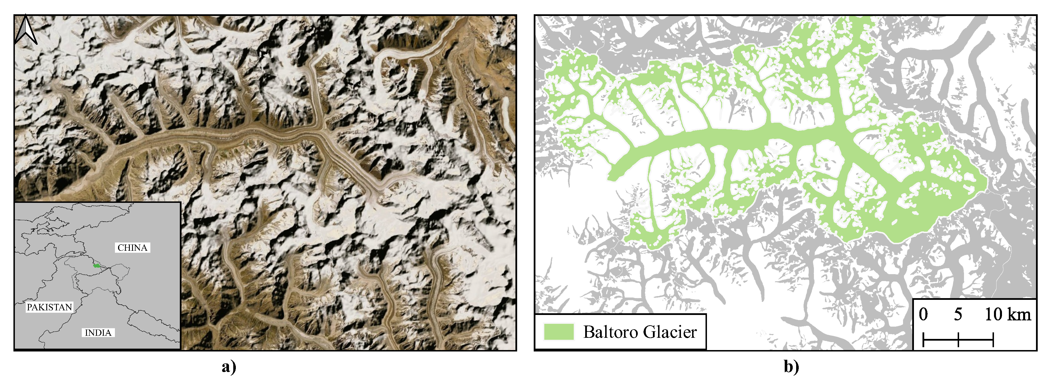
2.1. Data

Training deep neural networks usually requires a large number of labeled data. In this work, we have generated the labeled data by manual digitization of the surface water in the PlanetScope imagery with the assistance of Very High Resolution Satellite (VHRS) imagery from Google Earth and ESRI World Imagery basemaps. The aid of the VHRS imagery in the digitization process was essential because the precise mapping of lake boundary is difficult in PlanetScope imagery as compared to VHRS imagery. Mapping of supraglaical lakes is especially challenging due to smaller size, mixing with snow and cast shadows. The PlanetScope imagery with approximately daily coverage is available from the year 2017. Therefore, the selection of the sites in the HKKH region for digitization was based on the availability of the very high-resolution imagery from recent years during the summer to early winter months. Emphasis has been placed on including a variety of landscapes containing different glacial lake types. The PlanetScope imagery from the same date as the very high-resolution imagery was downloaded. In some cases, the PlanetScope imagery from different dates was used because PlanetScope imagery of the same date did not have complete coverage of the area of interest. An image is a mosaic of multiple PlanetScope scenes covering each location and in several cases, the mosaic consists of images from multiple satellites. When there was overlap between multiple PlanetScope scenes, data from only one scene were used for overlapping pixels. The locations of the digitized images are shown in Figure 2, while details are given in Table 1. Here, the PlanetScope Top of Atmosphere (TOA) radiance product was used. The total number of digitized polygons was 5177 in an area of approx. 4200 km 2 and the lakes area was approx. 71 km 2 . The minimum mapping unit was set to one pixel, which the digitizer can recognize as a water pixel in PlanetScope imagery. So, if there is a small water body visible in VHRS imagery but not recognizable as water pixel in PlanetScope imagery, it has been removed.
The errors in the ortho-rectification due to topography and the sensor orientation leads to the difference in the positions of the water pixels in the PlanetScope imagery and the VHRS imagery. While the errors due to sensor orientation can be modeled as a shift or an affine transformation, the distortions due to topographic errors can vary over the image and will depend on the angle of the image ray vector to the nadir. So, the higher the off-nadir angle, the higher can be the difference in the corresponding pixels in the VHRS image and the PlanetScope image. Thus, the shift in the digitized polygons was visually inspected and corrected by overlaying the polygons on the PlanetScope imagery. The NDWI and the false-color composites were also employed to help the digitizer in delineating the lake boundaries and determining the shift between the VHRS imagery and the PlanetScope imagery. Some samples of the digitized water bodies are shown in Figure 3.
The polygons created by the digitization process were used to generate a binary image mask in which the foreground pixels (‘1’) represent water while the background pixels (‘0’) represent non-water pixels. If the water polygon covers more than 50 % of the area of the pixel, then it was set to ‘1’. An important point to consider here is that all the pixels which belong to water should be ‘1’ in the output mask used for training the CNN. The water pixels belonging to the rivers and streams were difficult to delineate. Therefore, we have masked out the image pixels belonging to rivers and streams. The non-overlapping image tiles of size 256 × 256 were created from the PlanetScope labeled images, which resulted in 6555 tiles, out of which 20 % (1311) image tiles were selected as validation data and 20 % (1311) image tiles were selected as test data randomly.

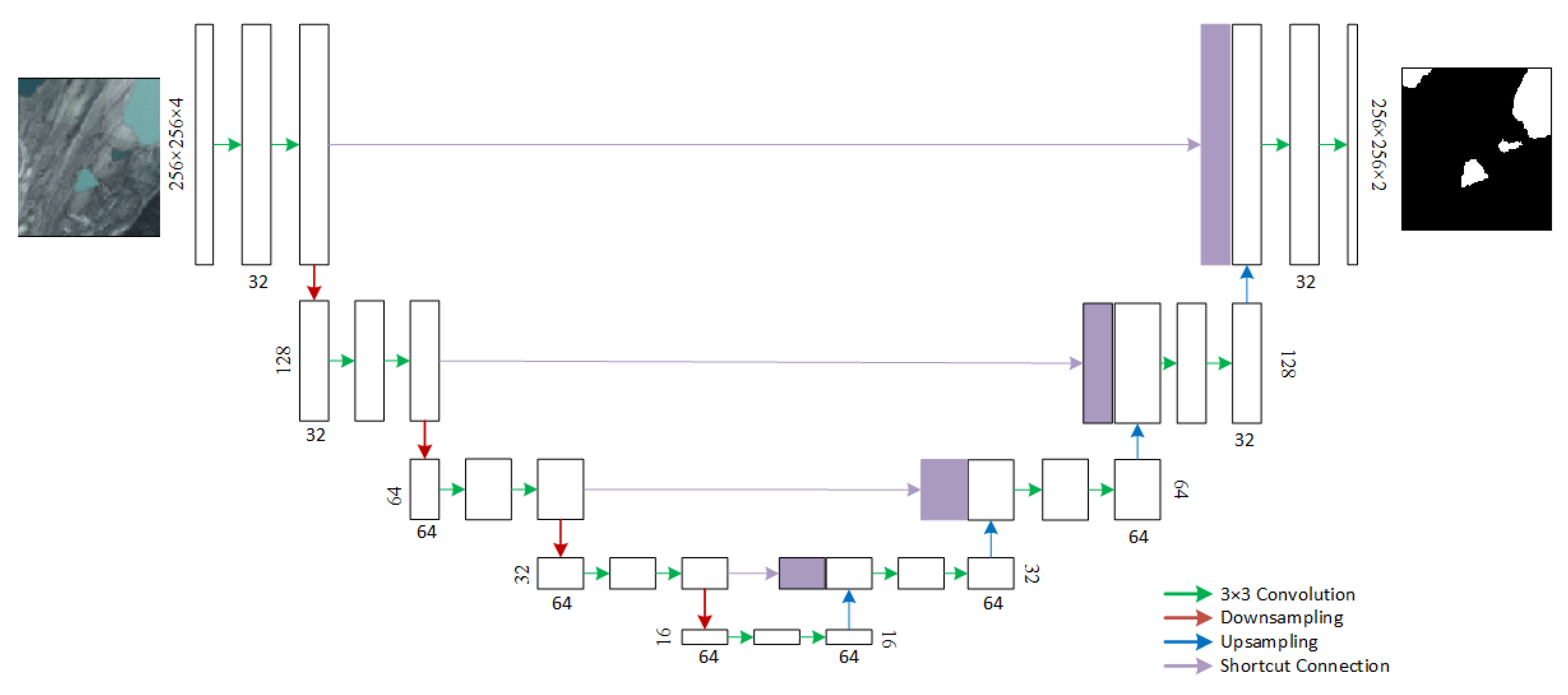
2.2. VGG U-Net Model

The CNN used in this work is based on the U-Net architecture, which contains encoder and decoder units connected using a shortcut connection, as shown in Figure 4. The encoder units consist of a typical VGG (network designed by the Visual Geometry Group) type [45] convolution layers followed by batch norm [46] and the ReLU (Rectified Linear Units) activations and then a max-pooling layer which downsamples the spatial size of the image. These encoder units extract multi-scale features from the input image. The decoder units then generate the segmentation mask from these features. The shortcut connection concatenates the features from the encoder unit with the corresponding decoder unit, which helps in better localization and information exchange using features at different stages of the network. The downsampling is performed by the maxpooling operation with a stride of 2, while the upsampling is performed by increasing the spatial size by a factor of 2 using the bilinear interpolation. We did not observe improvement by using transposed convolution layers, which can learn the upsampling coefficients. The number of feature maps for each convolution layer are shown in Figure 4. We experimented with several different network sizes and the network shown here was selected after evaluating models with different depth and width. We didn’t use the pre-trained VGG16 network in the U-Net due to its large size (138 million parameters), which results in overfitting. Our evaluation showed that relatively smaller networks (in terms of the number of parameters and memory footprint) showed better performance on this dataset.

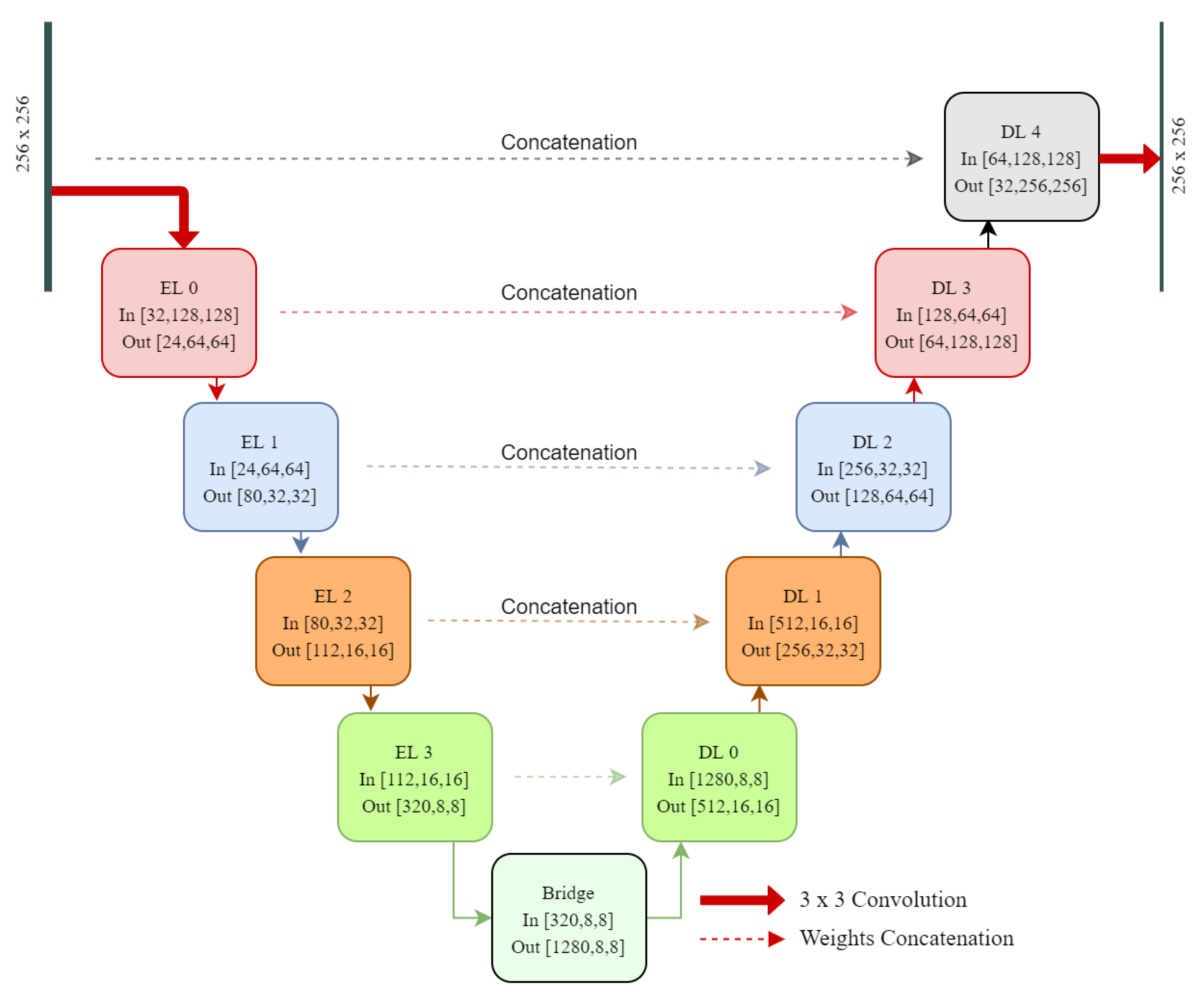
2.3. EfficientNet U-Net Model

It is often preferable to use a pre-trained model instead of using a customized model, as the pre-trained models are trained on large datasets, which reduces the training time as well as overfitting. For satellite imagery, models trained on datasets like Eurosat [47], BigEarthNet [48] and SpaceNet [43] can be used for transfer learning. However, to the best of our knowledge, no publically available pre-trained models exist for 4-bands PlanetScope imagery. Therefore, we used the pre-trained EfficientNet [49] as the backbone of the U-Net architecture as it has recently produced state-of-the-art results with fewer parameters and lesser training time. The EfficientNet is built upon the idea of uniformly scaling up the network size i.e., depth, width and resolution. This produces a family of networks known as EfficientNets. The baseline model with around five million parameters is model B0, while the largest model is B7, with 66 million parameters. The EfficientNet’s main building blocks are the inverted bottleneck block [50], which also contains squeeze-and-excitation networks [51]. We evaluated the EfficientNet models starting from the baseline model B0 to larger size models. We noticed that the larger models did not further improve accuracy. Therefore, we used EfficientNet B0 as the backbone of the U-Net architecture as shown in Figure 5. The decoder layers are similar to the original U-Net architecture. The first convolution layer of the EfficientNet was changed to incorporate 4-band PlanetScope imagery.

2.4. Training

The training was performed on an Nvidia RTX 2070 GPU with 8GB memory. The initial learning rate was set to 0.01, which was then reduced by a factor of 0.1 when the loss starts to plateau. The batch size was set to 16. The parameters of the convolution layers i.e., weights were initialized using He’s method [52] in the customized U-Net model and the decoder part of the EfficientNet U-Net. The input image tiles are randomly picked from the training dataset. As the number of water pixels were fewer then the background pixels, we used weighted loss in which higher weight was assigned to water pixels during loss computation. The data augmentation was performed using random flipping and mirroring and brightness change. The hyper parameter weight decay and momentum had values 0.0005 and 0.9, respectively. The network has been trained for 100 epochs. We further utilized label smoothing [53,54], which showed improvement in the accuracy of the network. The performance of the network was evaluated on validation data after each epoch and the trained network with the best performance on the validation data was chosen for evaluation on the test dataset. The inference using the trained network was performed by extracting overlapping patches of size 256 × 256 from the PlanetScope images. The border pixels are ignored for each patch. The class labels were assigned by summing up the individual probabilities from each overlapping patch. The network design, training and inference are performed using PyTorch library [55]. The inference on a complete PlanetScope scenes took less than a minute on RTX2070 GPU.

2.5. Random Forest

Random Forest (RF) has been a popular classifier for the detection of glacial lakes in remote sensing imagery [56,57,58]. Therefore, to compare the performance of the CNN, RF Classifier was trained to classify PlanetScope images into water and background classes. An RF classifier builds an ensemble of trees by a random subset of the samples and the features. Each tree was built using the Gini Index or the Information Gain criterion. The training data available were rather large; therefore, we tested with a different number of samples for training the RF classifier. After evaluation, we chose 20,000 samples of each class for building the RF classifier. The number of trees was set to 200. Out-of-bags samples were used for validation. The input to the classifier consists of 4-bands of each pixel as well as the normalized difference of band 4 with the other three bands. After training, the RF classifier was used to predict the class label for each pixel of the test images.

2.6. Support Vector Machines

Support vector machine (SVM) classifier is a maximum margin classifier, which computes the decision boundary by keeping maximum distance from the support vectors or the samples closest to the decision boundary. SVM has been a popular machine learning classifier, widely used in different applications. The nonlinear decision boundary in SVM is computed using the kernel trick, which implicitly performs the transformation of the samples into a higher-dimensional space as well as the dot product of the samples. Similar to the RF classifier, we used normalized differences of band 4 with the other three bands as additional features as inputs for the classifier. The number of samples, kernel function and the gamma value of the kernel function were tuned to achieve best performance on the test data. Using fewer samples of water pixels in comparison to background pixels increased the accuracy of the classifier. After evaluation, we chose 1000 samples (pixels) of water and 5000 samples of background. The third degree polynomial kernel with gamma value 1 was selected after evaluation. The training and prediction of the SVM classifier was done using LibSVM [59].

2.7. Lake Area Uncertainty

The uncertainty in the estimated area of the lakes depends on the number of pixels on the perimeter of the lake. Here, we assumed ± 1 pixel uncertainty at the perimeter of the lake. If G is the spatial resolution of the image and P is the perimeter of the lake, then the uncertainty in the lake area is computed using the formula [60]:
A e r ( 1 σ ) = 0.6872 × P G × G 2 .

2.8. Evaluation Metrics

The evaluation on the test data was performed using the Precision (Equation (2)), Recall (Equation (3)), F1-Score (Equation (4)) and Kappa Coefficient (Equation (5)). The F1-Score is the harmonic mean of Precision and Recall. Precision and Recall are computed using the True Positives (TP), False Positives (FP) and False Negatives (FN), which can be computed using the confusion matrix.
P r e c i s i o n = T P T P + F P
R e c a l l = T P T P + F N
F 1 S c o r e = 2 × P r e c i s i o n × R e c a l l P r e c i s i o n + R e c a l l
K a p p a C o e f . = N × x i i ( x i + × x + i ) N 2 ( x i + × x + i )
The Kappa Coef. was also computed using the confusion matrix, where N is the total number of pixels, x i i are the diagonal elements of the confusion matrix, x i + and x + i are the sum of the rows and columns of the confusion matrix. These evaluation metrics are computed by taking in to account all the pixels of the 1311 tiles of the test data. Thus, a single confusion matrix is computed using all pixels of the test data and the evaluation metrics are then computed using this confusion matrix.

3. Results

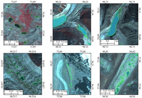
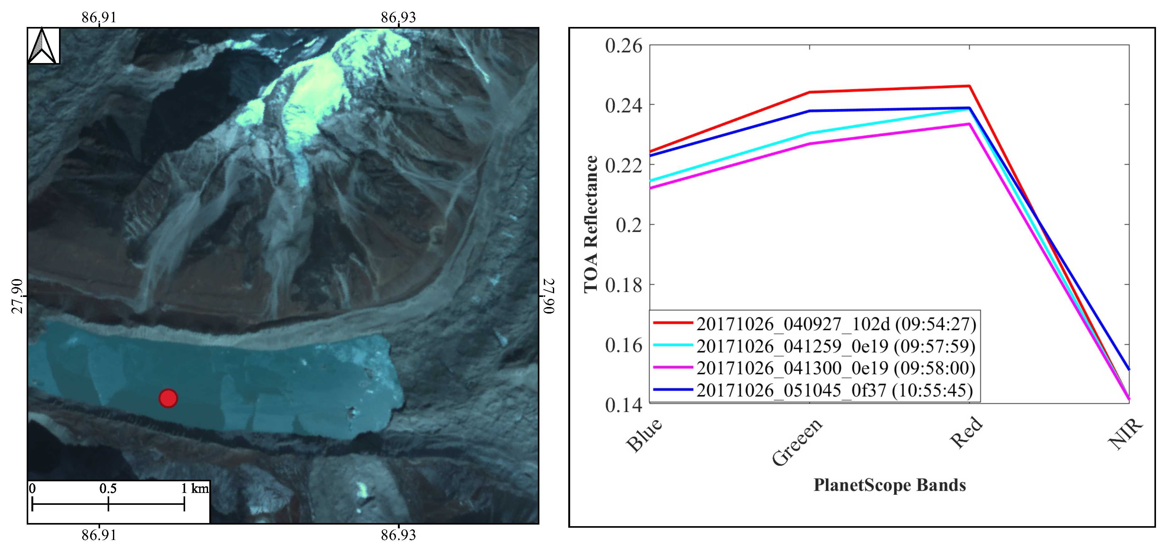
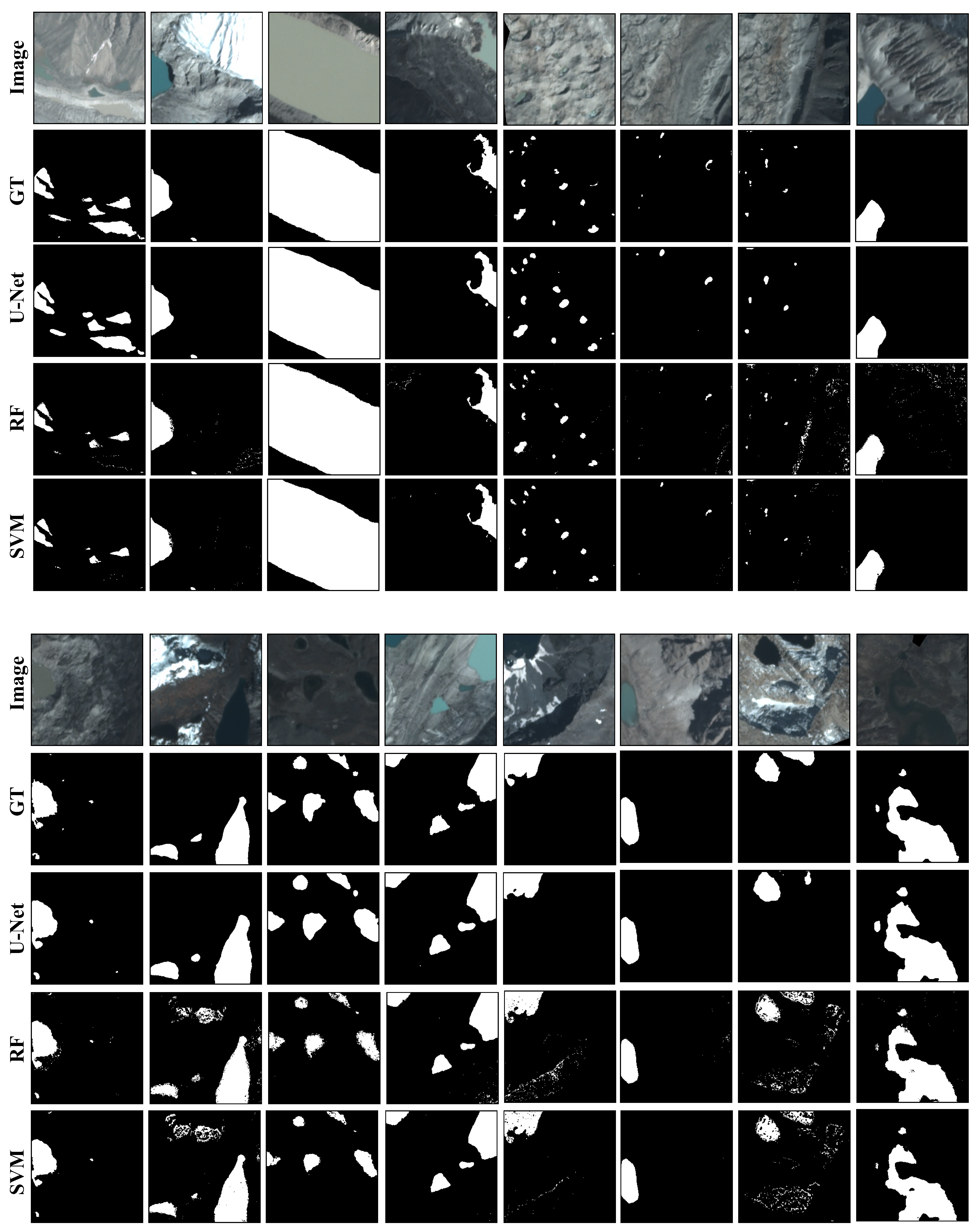
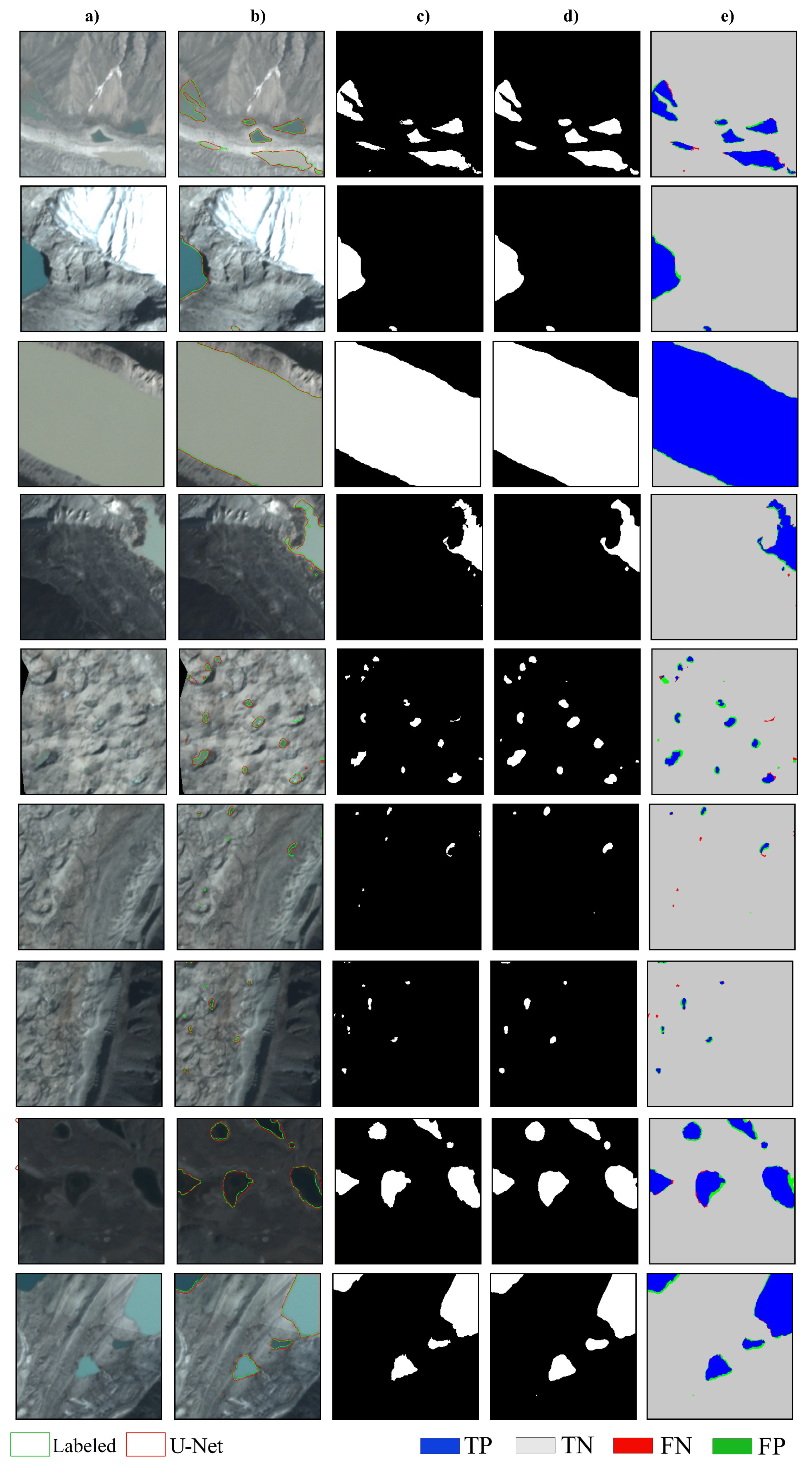
3.1. Evaluation on the Test Data

The trained U-Net models (VGG U-Net and the Efficient U-Net), RF and SVM classifiers were used for prediction on the test data. The accuracies of the models are evaluated using metrics Precision, Recall, F1 Score and the Kappa Coef. as given in Table 2. The EfficientNet U-Net model achieved the highest F1 Score and Kappa Coef. of 0.936 and 0.935, respectively, while the VGG UNet achieved an F1 Score and Kappa Coef. of 0.930 and 0.929, respectively. Due to the better performance of the EfficientNet U-Net, we further used this model for inference on PlanetScope images. The RF classifier achieved an F1 Score and Kappa Coef. of 0.754, while SVM achieved an F1 Score of 0.775 and Kappa Coef. of 0.771 This shows that the deep learning models achieve significantly better accuracy as compared to the RF and SVM classifiers. The comparison of the ground truth polygons, EfficientNet U-Net and the RF classifier are shown in Figure 6. There is a significant number of false positives in the shadows and an underestimation of the lake boundary by the random forest classifier as shown in Figure 6. For a visual comparison, the predicted binary masks are converted to polygons and compared with the ground truth polygons as shown in Figure 7. The results show that in the majority of the lakes, the predicted, as well as the ground truth polygons, overlap to a large extent. The smaller supraglacial ponds have occasionally been missed by the U-Net model.

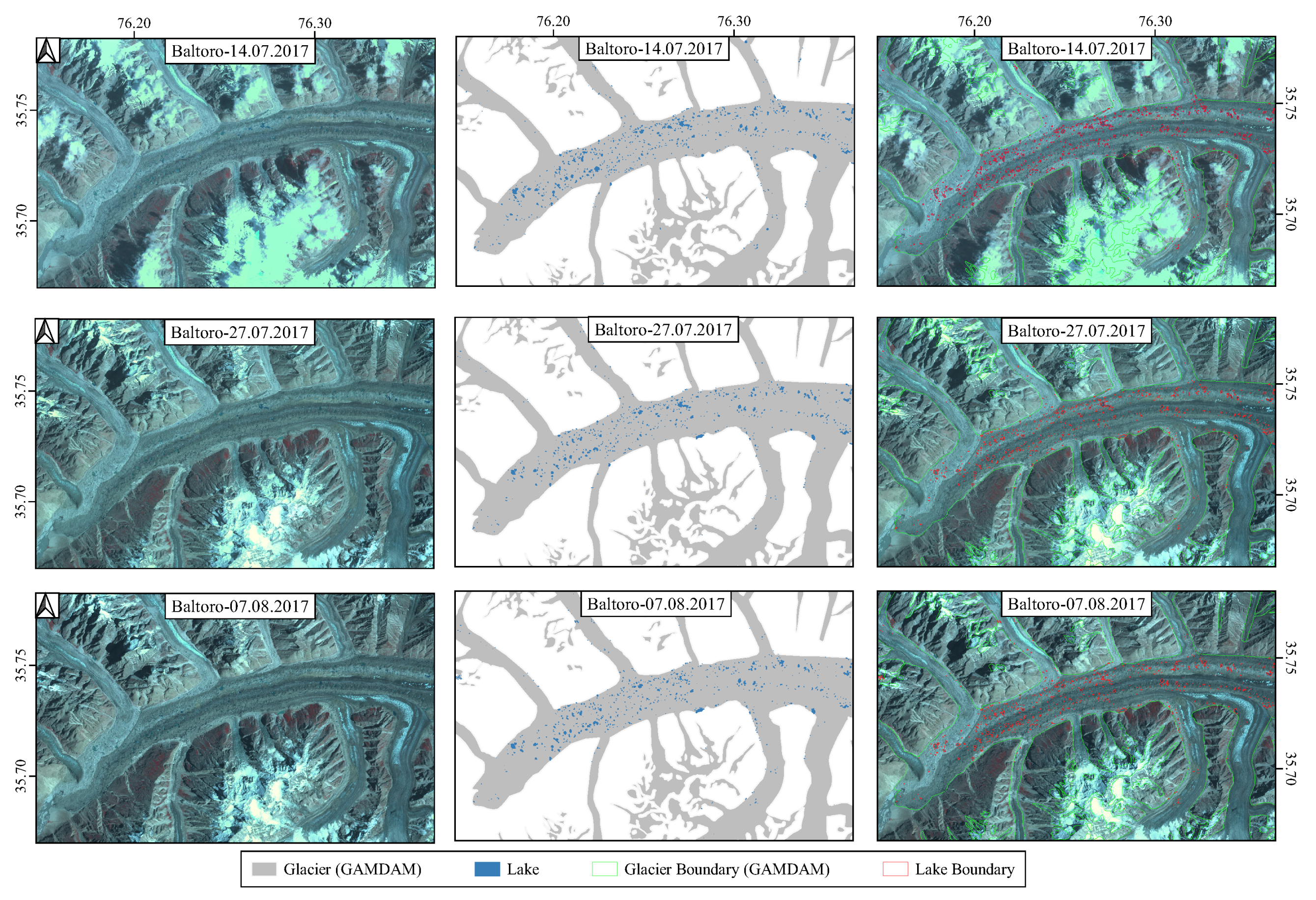
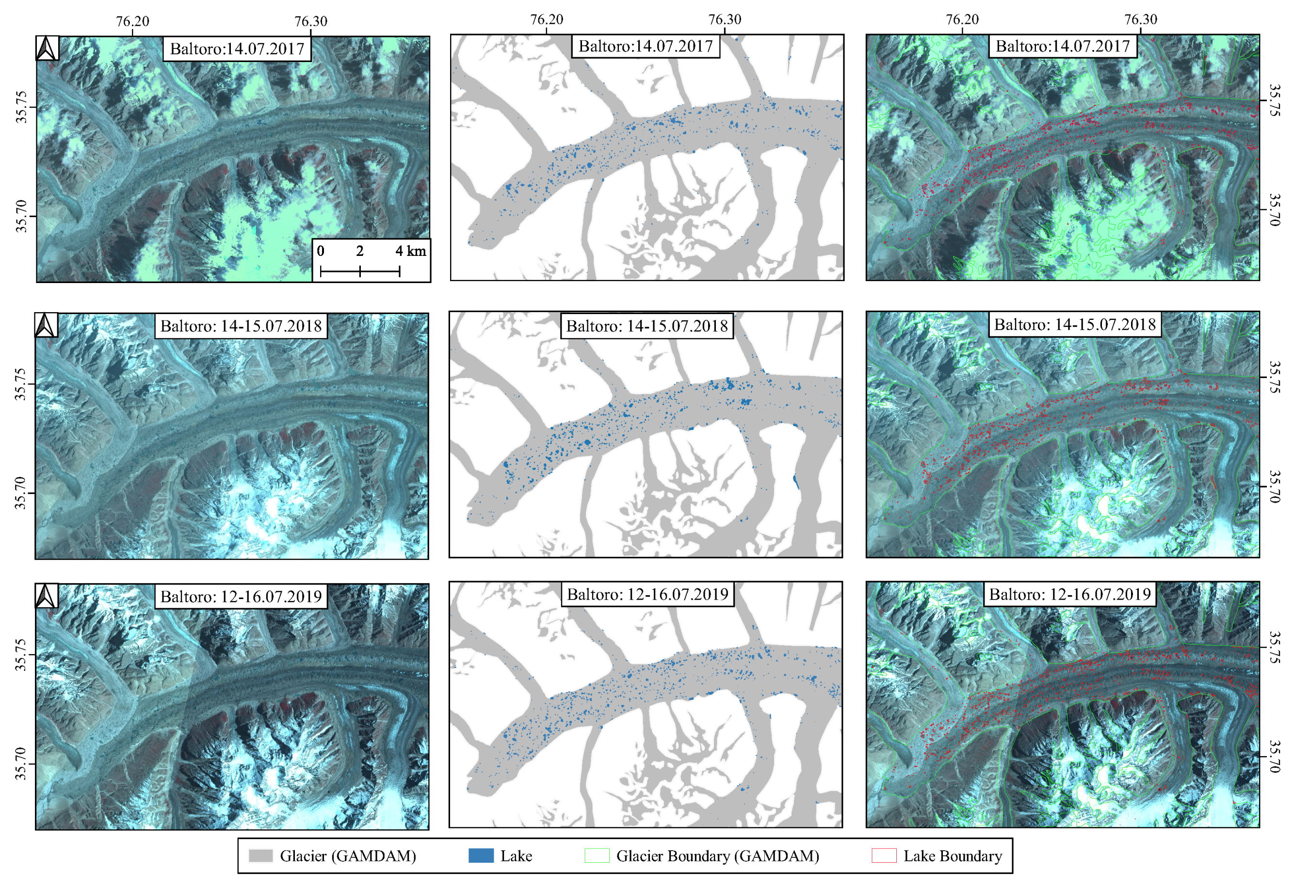
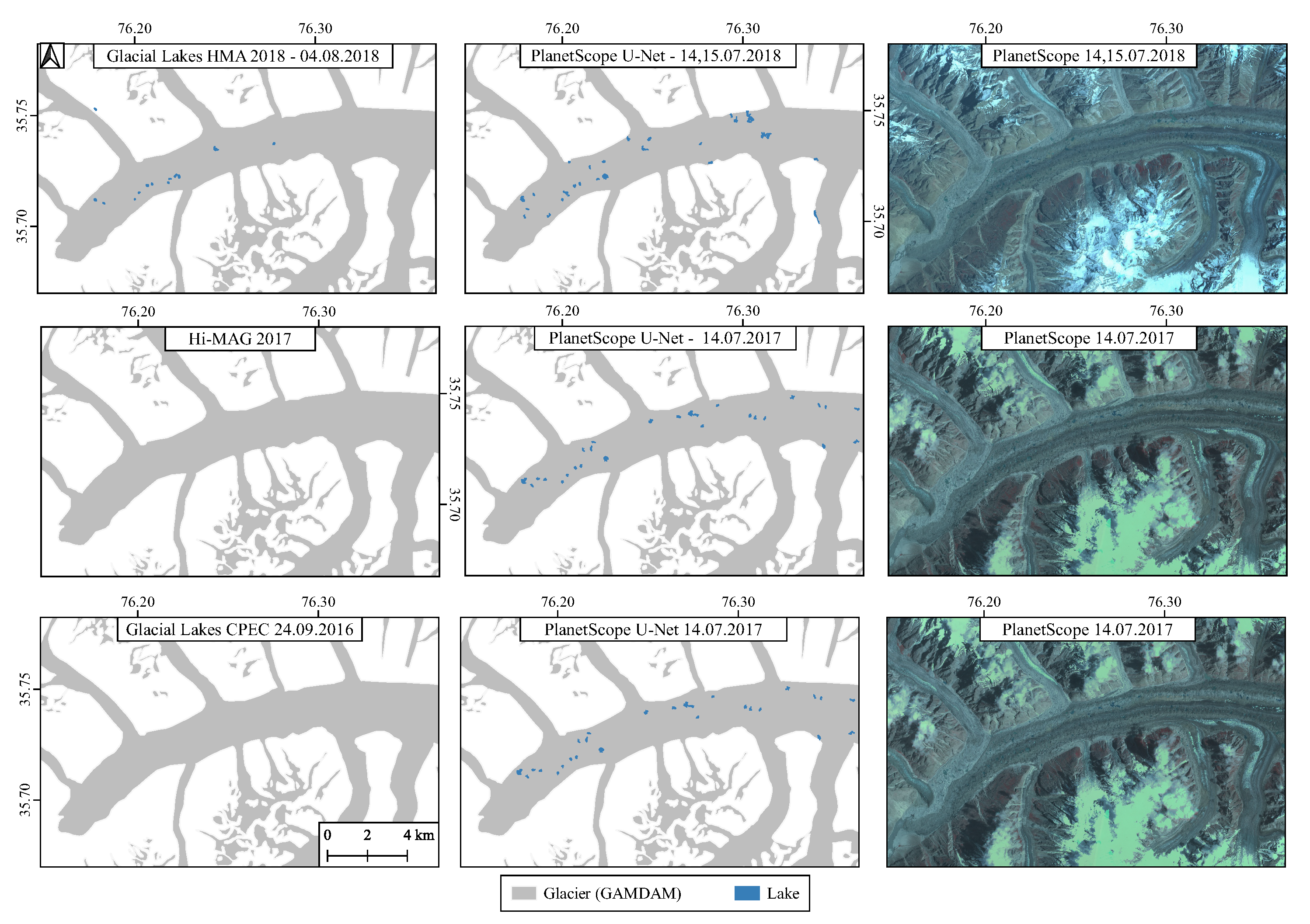
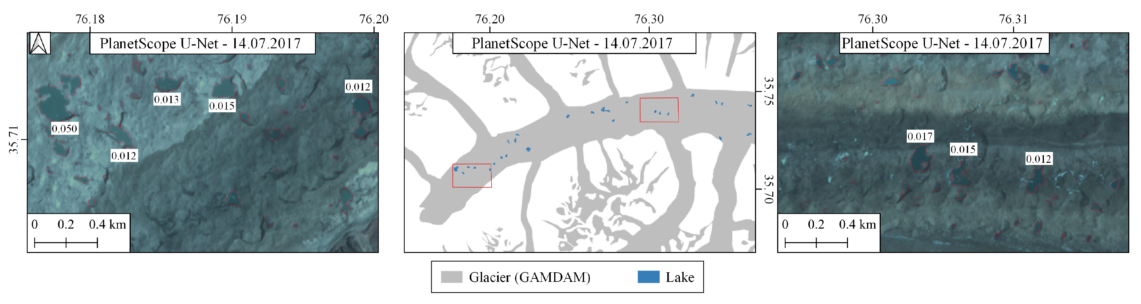
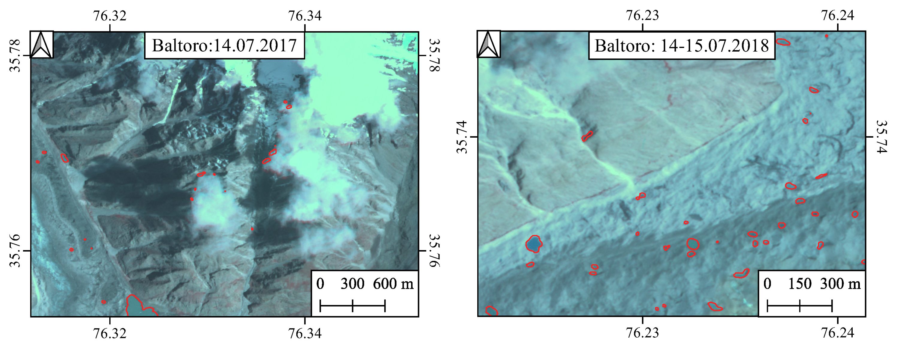
3.2. Mapping Supraglacial Lakes on the Baltoro Glacier and Comparison with Existing Glacial Lake Inventories

We then mapped supraglacial lakes on the Baltoro glacier (Figure 8) and compared the results with existing glacial lake inventories of the recent past having an overlap with the PlanetScope data availability. Figure 9, shows the variations in the supraglacial lakes within a time difference of around two weeks. Visual analysis shows several differences in the supraglacial lakes within a short time difference. Figure 10 shows supraglacial lakes with a time difference of one year. The variations over a year were much more significant and some relatively larger supraglacial lakes also show variations in terms of number and size. The trained U-Net model was able to automatically extract the majority of the supraglacial lakes. The sizes of the supraglacial lakes on the Baltoro glacier mapped using PlanetScope imagery of different dates are given in Table 3. We then used the following inventories for comparison: (1) glacial lakes inventory of High Mountain Asia [36], (2) A dataset of glacial lakes in High Mountain Asia (Hi-MAG) from 2008 to 2017 [61] and (3) glacial lakes in the China–Pakistan Economic Corridor (CPEC) [62]. These three inventories have been derived from Landsat-8 imagery (recent years). The minimum mapping area of (1) is 0.0054 km 2 (2) is 0.0081 km 2 and (3) is 0.01 km 2 . These inventories have relied on manual [36] or semi-automatic [61,62] techniques for delineation of glacial lakes using Landsat imagery. The comparison of the supraglacial lakes is presented in Figure 11 and Table 4, which shows that several lakes have been missed in the inventory [36] and the inventories [61,62] have not detected lakes on the Baltoro glacier even though the data in Table 3 suggest that a significant number of lakes have an area greater than the minimum mapping area of these inventories. Figure 12 shows the area along with each lake having area > 0.01 km 2 . Here, it should be mentioned that the entire Earth landmass is currently not covered by the PlanetScope daily imagery. The area acquired changes due to the change in the number of operational satellites as well as due to the position and orientation of the satellites. The entire area of the Baltoro glacier is not covered by a single PlanetScope scene and several scenes were required to cover the entire Baltoro glacier. Therefore, due to partial coverage, we could not use the PlanetScope imagery from the same date as used in these inventories.

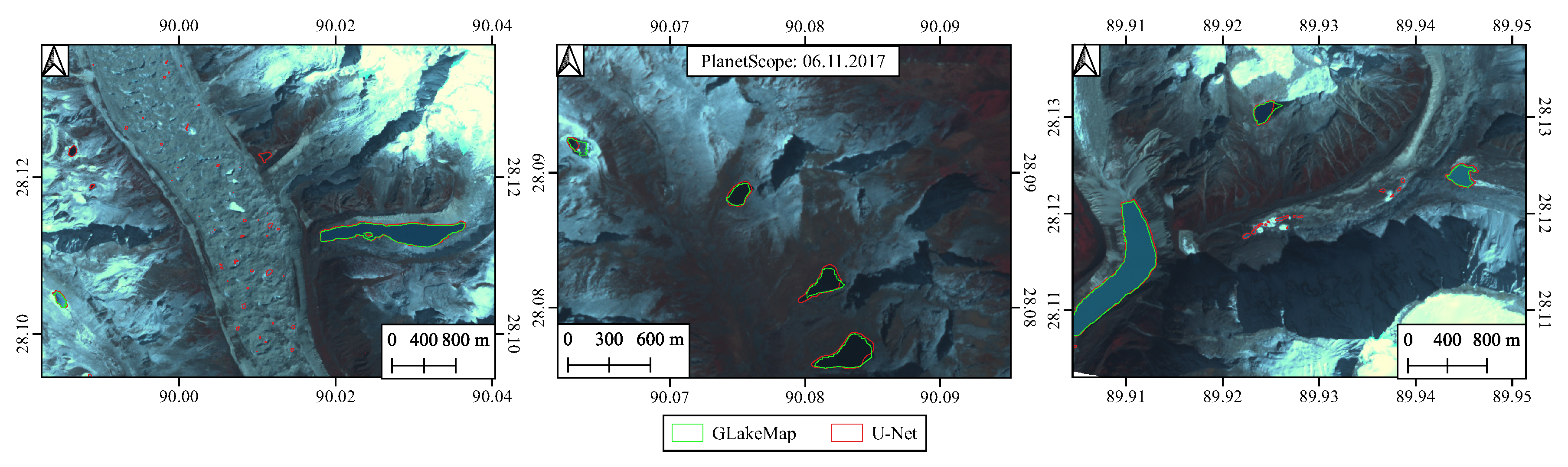
3.3. Comparison with GLakeMap Automated Pipeline

We then visually compare the glacial lakes mapping with the results from “GLakeMap” automated pipeline for mapping glacial lakes using Sentinel-1 and Sentinel-2 data [56]. The GLakeMap uses rule-based segmentation to extract segments from the Sentinel-1/2 images and DEM data and then classifies those segments using a Random Forest classifier. The minimum mapping area in GLakeMap is 0.01 km 2 and the method was tested on eight different sites across the globe. Figure 13 shows the comparison of the outlines from GLakeMap (Sentinel-1/2) and the U-Net (PlanetScope) models over an area in Bhutan. The relatively larger lakes are mapped quite well by both U-Net and GLakeMap. However, the U-Net model has also extracted smaller lakes quite well.

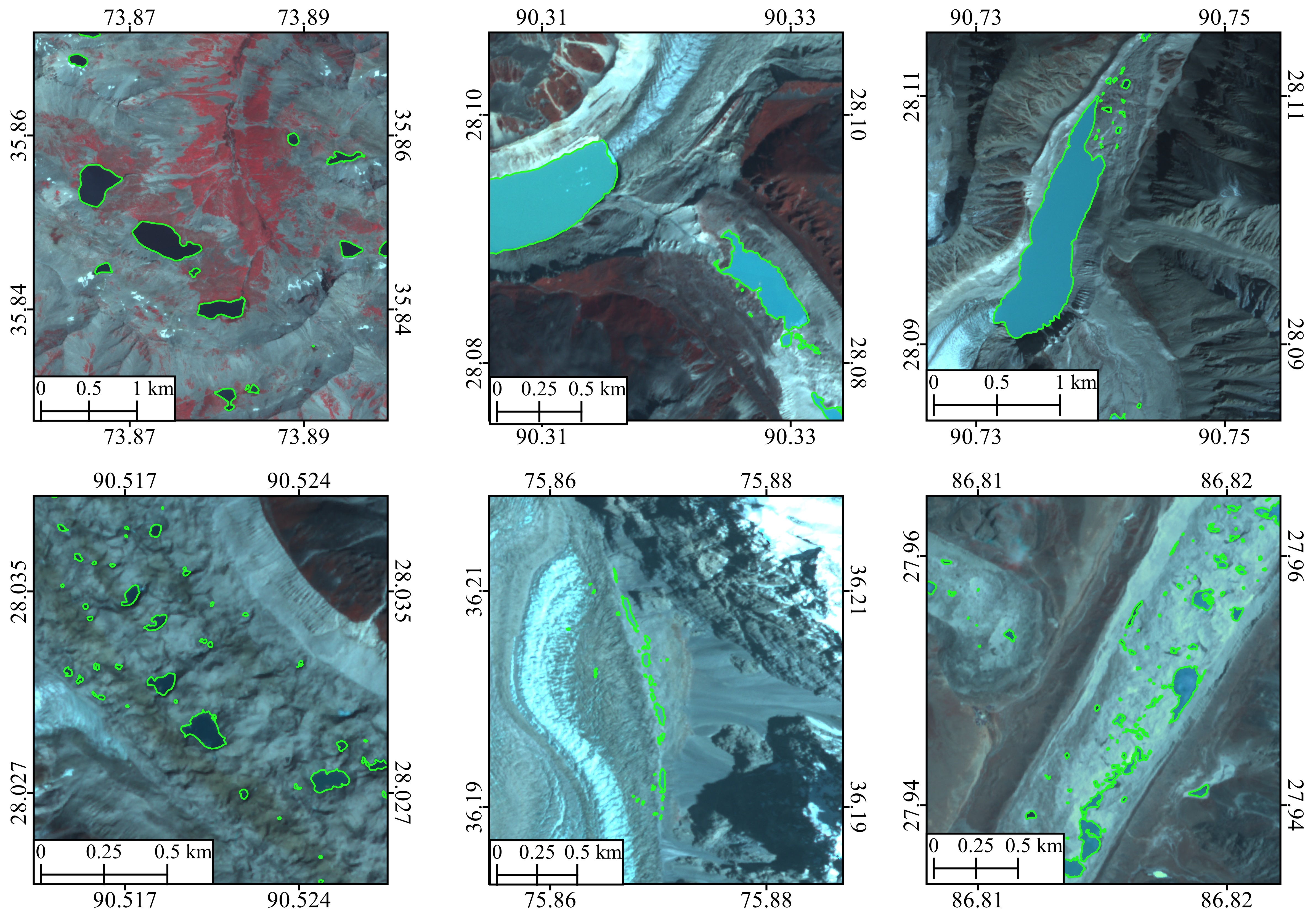
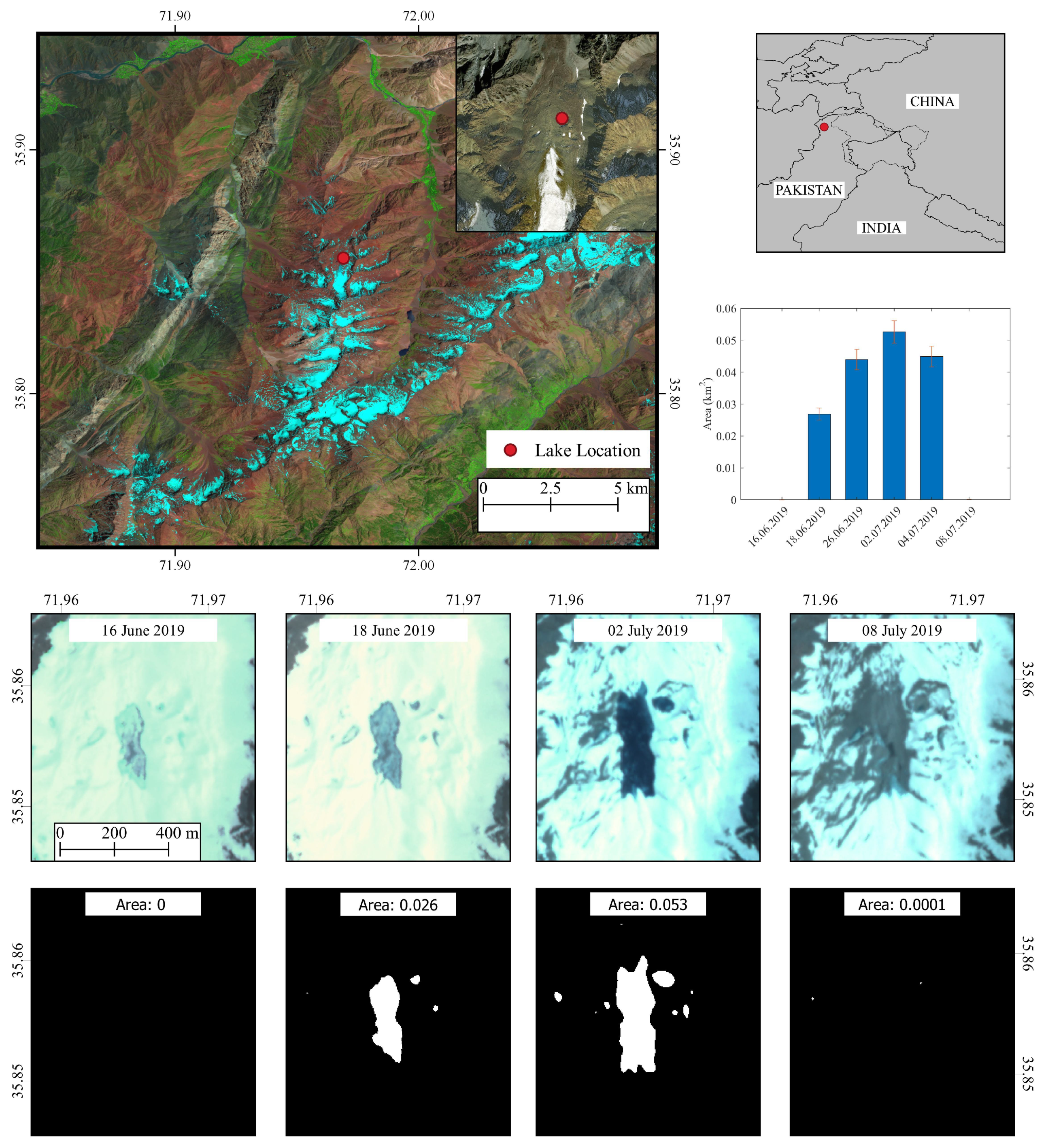
3.4. Examples of Lake Outburst and Lake Area Mapping

The trained U-Net model was then qualitatively evaluated on PlanetScope images of two different glacial lakes time-series imagery. First, we considered the GLOF event in the Chitral district of the Hindu Kush Range in July 2019 caused by a newly formed glacial lake on the end moraine of the Rogheli glacier at an elevation of around 4500 m as shown in Figure 14. The PlanetScope imagery shows the formation of the lake which is detected by the trained model in the PlanetScope image from 18 June 2019 as shown in Figure 14. The GLOF event occurred on 7 July 2019 at around 5:00 pm [7]. The PlanetScope image from 8 July 2019 shows the lake has drained. The maximum surface area of the lake extracted by the deep learning model is 0.052 km 2 . The early detection of the lake in such a scenario is challenging due to a mixture of frozen and meltwater. The training data used in this work contained some similar instances in which the lake contains partially frozen water. Therefore, the deep learning model was able to extract the lake in the PlanetScope scene of 18 June 2019. In the earlier scenes, the formation of the lake can be visually identified but wasn’t detected by the U-Net.
The trained U-Net is then tested on the PlanetScope scenes of the glacial lake formed by the Shishper glacier surge. The Shishper glacier in the Karakoram range started to surge in Spring 2018 with maximum velocity reaching up to 20 m/day. The surging glacier blocked the outflow of the Muchowar glacier resulting in the formation of the lake as shown in Figure 15. The lake grew to a size of around 0.18 km 2 in May/June 2019. The lake drained in late June 2019 through a subglacial stream, causing moderate flooding in the downstream area but the damage was mitigated by protection walls built by the authorities anticipating the potential flood. The surface of the lake as shown in Figure 15, partially contained debris and ice, which makes it difficult to precisely map surface water. Visual analysis of the results show that the U-Net is able to extract surface water and separate it from debris reasonably well.

4. Discussion

The results presented above show that the deep learning-based model can be employed in practice for the automatic extraction of glacial lakes in PlanetScope imagery. The results show that even with the variations in the images from different PlanetScope satellites, the deep learning model was able to generalize and perform well on the unseen PlanetScope images of a different area. We have observed some false positives on pixels on the cloud edges during our evaluation as shown in Figure 16. This can perhaps be solved by using the cloud masks provided in the PlanetScope supplementary data or to include clouds in the training data. False positives were also observed due to cast shadows in the images of Baltoro and Shishper glacier. We have also observed that some lakes with muddy brown color were not extracted by the U-Net, which shows that the training data need expansion to include all possible types of lakes that may occur. Another important point to consider here is that the larger lakes are sometimes easier to map than the relatively smaller lakes and the larger lakes have a higher weightage on the resulting metrics because it contains more pixels i.e., the evaluation metrics are influenced more by the larger lakes. Therefore, one may consider computing evaluation metrics for different lake sizes.
In the generation of the labeled data, the relative displacement of water bodies between the VHRS imagery and PlanetScope imagery was a major issue and required a lot of time to correct. Due to a lower resolution of the PlanetScope imagery, it was very difficult sometimes to determine this shift and as a result, even the labeled data will have some inaccuracies. When generating the labeled data, delineating the boundary of very shallow water bodies is also very difficult and the delineation is dependent on the interpretation of the digitizer. Some small lakes were missed in the original digitization process, but the trained U-Net was able to extract those lakes. Thus, we used the U-Net model to track errors in the digitization process and correct those errors and train the network again. The precise delineation of the supraglacial lakes is very challenging due to their smaller size, mixture with snow and debris and cast shadows. The changes in the extent of the supraglacial lakes within a short time period also makes it difficult to use and compare images of different dates.
The GLOF event in the Chitral district shows the importance of frequent mapping of the glacial lakes because new lakes can be formed, which may suddenly drain after some time. Such events have occurred in the past and it is imperative to monitor such situations using remote sensing datasets. The automation of the whole process is essential as this region spreads over a large area and it is not possible to visually inspect the whole area. It should be mentioned that the occurrence of GLOF depends on various factors. In this work, we only attempted to map the lake area in a dynamic scene without any consideration of the outburst probability. The damming of the glacial lakes in one of the important factors in designating a glacial lake as a potentially dangerous lake. Such classification of the lakes was also not studied in this work.
In the case of the Shishper glacier surge the volume of the lake changed over time and frequent mapping helps to determine the water quantity and compute simulations of water discharge and possible flood scenarios. It should be mentioned that, due to the presence of clouds, no PlanetScope scenes were available on the day the lake in Chitral and Shishper drained. Therefore, due to the limited availability of cloud-free images in parts of HKKH, any solution to monitor surface water from remote sensing satellites should also incorporate both optical and microwave satellite data in the future, especially due to the recent progress by the commercial companies to develop a constellation of Synthetic Aperture Radar (SAR) satellites [64]. The inclusion of the microwave remote sensing data for glacial lakes mapping is inevitable.
The labeled data generated in this work covered only the HKKH region. Assessing the transferability of the model to a different study area is also interesting. Here, we map the glacial lakes in the Peruvian Andes using the PlanetScope imagery and the trained U-Net model as shown in Figure 17. For a comparison, the glacial lake outlines of Cordillera Blanca (Peru) [65], which have been derived from visual interpretation of satellite imagery are also shown as a reference. A visual analysis of the results shows that the trained U-Net model generalizes well to the other areas.

5. Conclusions

In this paper, we explored the potential of PlanetScope imagery for glacial lakes mapping in HKKH. Due to inherent difficulties in mapping surface water in mountainous regions, deep learning-based model was used for mapping of surface water. A dataset consisting of more than 5000 water bodies covering an area of approx. 71 km 2 in eight different sites in HKKH was created. The results on the test images showed that the U-Net model with EfficientNet backbone achieved higher accuracy (F1 Score of 0.936) than the U-Net with VGG style layers, RF and SVM classifiers. The results further showed that there are few false positives in the predicted water masks while the majority of the water pixels are correctly identified by the trained model. The trained U-Net model is then used for mapping the supraglacial lakes on Baltoro glacier and the results showed that U-Net model extracted more lakes than the recently published glacial lakes inventories. This shows that even with 4-bands imagery from PlanetScope small satellites, glacial lakes can be reliably extracted. These results are especially significant as most of the earlier work has relied on multispectral remote sensing imagery with a higher number of bands. A comparison with the GLakeMap results also showed that the U-Net model can detect glacial lakes using PlanetScope imagery with high accuracy. The higher spatial and temporal resolution of PlanetScope imagery can significantly improve the mapping of the glacial lakes. The trained U-Net was then evaluated on the PlanetScope time-series imagery of two different glacial lakes with varying water surface area. The changing water area was well-mapped by the U-Net model in PlanetScope scenes. This shows that the trained model also works well on PlanetScope images, which were not part of the original digitized dataset. The GLOF event in the Chitral district shows the importance of frequent mapping of the glacial lakes. The newly formed ice/moraine dammed lake on the Rogheli glacier suddenly drained, causing significant damage to the infrastructure downstream. Early detection of the lake in such a scenario would help expedite the mitigation efforts, which may reduce the damage due to the outburst flood. Planet Labs plan to launch PlanetScope satellites with 8-band imaging capabilities in 2020, this may further improve the accuracy of glacial lake mapping in PlanetScope imagery but will require training data from the newer generation satellites.

Author Contributions

Sajid Ghuffar, Nida Qayyum and Imran Shahid designed the study, Nida Qayyum and Sajid Ghuffar created the dataset. Nida Qayyum, Sajid Ghuffar, Hafiz Mughees Ahmad and Adeel Yousaf processed the data and implemented machine learning algorithms. All authors contributed to the paper writing and validation. All authors have read and agreed to the published version of the manuscript.

Funding

This research was supported by the International Foundation for Science (IFS) and COMSTECH grant Ref. No. W/5805-1.

Acknowledgments

We thank Tobias Bolch and Sonam Wangchuk from University of St Andrews, UK for sharing the GLakeMap results and for their feedback and comments. We would also like to thank the authors of the glacial lake inventories [36,61,62] and Adam Emmer, University of Graz, Austria for sharing their datasets. We thank Akiko Sakai from Ngoya University, Japan for providing the GAMDAM inventory data. We thank Planet Labs for providing access to their daily imagery through the education and research program.

Conflicts of Interest

The authors declare no conflict of interest.

References

  1. Shugar, D.H.; Burr, A.; Haritashya, U.K.; Kargel, J.S.; Watson, C.S.; Kennedy, M.C.; Bevington, A.R.; Betts, R.A.; Harrison, S.; Strattman, K. Rapid worldwide growth of glacial lakes since 1990. Nat. Clim. Chang. 2020, 1–7. [Google Scholar] [CrossRef]
  2. Brun, F.; Berthier, E.; Wagnon, P.; Kääb, A.; Treichler, D. A spatially resolved estimate of High Mountain Asia glacier mass balances from 2000 to 2016. Nat. Geosci. 2017, 10, 668. [Google Scholar] [CrossRef] [PubMed]
  3. Yao, X.; Liu, S.; Han, L.; Sun, M.; Zhao, L. Definition and classification system of glacial lake for inventory and hazards study. J. Geogr. Sci. 2018, 28, 193–205. [Google Scholar] [CrossRef] [Green Version]
  4. Rounce, D.; Watson, C.; McKinney, D. Identification of hazard and risk for glacial lakes in the Nepal Himalaya using satellite imagery from 2000–2015. Remote Sens. 2017, 9, 654. [Google Scholar] [CrossRef] [Green Version]
  5. Bolch, T.; Buchroithner, M.F.; Peters, J.; Baessler, M.; Bajracharya, S. Identification of glacier motion and potentially dangerous glacial lakes in the Mt. Everest region/Nepal using spaceborne imagery. Nat. Hazards Earth Syst. Sci. 2008, 8, 1329–1340. [Google Scholar] [CrossRef] [Green Version]
  6. Richardson, S.D.; Reynolds, J.M. An overview of glacial hazards in the Himalayas. Quat. Int. 2000, 65, 31–47. [Google Scholar] [CrossRef]
  7. Chitral, D. Golain, Chitral GLOF Event; Deputy Commissioner: Lower Chitral, Pakistan, 2019. [Google Scholar]
  8. Steiner, J.F.; Kraaijenbrink, P.D.; Jiduc, S.G.; Immerzeel, W.W. Brief communication: The Khurdopin glacier surge revisited–extreme flow velocities and formation of a dammed lake in 2017. Cryosphere 2018, 12, 95–101. [Google Scholar] [CrossRef] [Green Version]
  9. Rana, A.S. Risk Assessment of Khordopin Glacier Surge and Glacier Dammed Lake Formation; Pakistan Meteorological Department: Islamabad, Pakistan, 2017.
  10. Ghuffar, S. DEM generation from multi satellite PlanetScope imagery. Remote Sens. 2018, 10, 1462. [Google Scholar] [CrossRef] [Green Version]
  11. Bhambri, R.; Watson, C.S.; Hewitt, K.; Haritashya, U.K.; Kargel, J.S.; Shahi, A.P.; Chand, P.; Kumar, A.; Verma, A.; Govil, H. The hazardous 2017–2019 surge and river damming by Shispare Glacier, Karakoram. Sci. Rep. 2020, 10, 1–14. [Google Scholar] [CrossRef] [Green Version]
  12. Sivanpillai, R.; Miller, S.N. Improvements in mapping water bodies using ASTER data. Ecol. Inform. 2010, 5, 73–78. [Google Scholar] [CrossRef]
  13. Boschetti, M.; Nutini, F.; Manfron, G.; Brivio, P.A.; Nelson, A. Comparative analysis of normalised difference spectral indices derived from MODIS for detecting surface water in flooded rice cropping systems. PLoS ONE 2014, 9, e88741. [Google Scholar] [CrossRef]
  14. Du, Y.; Zhang, Y.; Ling, F.; Wang, Q.; Li, W.; Li, X. Water bodies mapping from Sentinel-2 imagery with modified normalized difference water index at 10-m spatial resolution produced by sharpening the SWIR band. Remote Sens. 2016, 8, 354. [Google Scholar] [CrossRef] [Green Version]
  15. Du, Z.; Li, W.; Zhou, D.; Tian, L.; Ling, F.; Wang, H.; Gui, Y.; Sun, B. Analysis of Landsat-8 OLI imagery for land surface water mapping. Remote Sens. Lett. 2014, 5, 672–681. [Google Scholar] [CrossRef]
  16. Wessels, R.L.; Kargel, J.S.; Kieffer, H.H. ASTER measurement of supraglacial lakes in the Mount Everest region of the Himalaya. Ann. Glaciol. 2002, 34, 399–408. [Google Scholar] [CrossRef] [Green Version]
  17. Planet Team. Planet Application Program Interface: In Space for Life on Earth; Planet Team: San Francisco, CA, USA, 2017. [Google Scholar]
  18. Cooley, S.W.; Smith, L.C.; Stepan, L.; Mascaro, J. Tracking dynamic northern surface water changes with high-frequency planet CubeSat imagery. Remote Sens. 2017, 9, 1306. [Google Scholar] [CrossRef] [Green Version]
  19. Kääb, A.; Altena, B.; Mascaro, J. River-ice and water velocities using the Planet optical cubesat constellation. Hydrol. Earth Syst. Sci. 2019, 23, 4233–4247. [Google Scholar] [CrossRef] [Green Version]
  20. Poursanidis, D.; Traganos, D.; Chrysoulakis, N.; Reinartz, P. Cubesats allow high spatiotemporal estimates of satellite-derived bathymetry. Remote Sens. 2019, 11, 1299. [Google Scholar] [CrossRef] [Green Version]
  21. Niroumand-Jadidi, M.; Bovolo, F.; Bruzzone, L.; Gege, P. Physics-based Bathymetry and Water Quality Retrieval Using PlanetScope Imagery: Impacts of 2020 COVID-19 Lockdown and 2019 Extreme Flood in the Venice Lagoon. Remote Sens. 2020, 12, 2381. [Google Scholar] [CrossRef]
  22. Wicaksono, P.; Lazuardi, W. Assessment of PlanetScope images for benthic habitat and seagrass species mapping in a complex optically shallow water environment. Int. J. Remote. Sens. 2018, 39, 5739–5765. [Google Scholar] [CrossRef]
  23. McFeeters, S.K. The use of the Normalized Difference Water Index (NDWI) in the delineation of open water features. Int. J. Remote Sens. 1996, 17, 1425–1432. [Google Scholar] [CrossRef]
  24. Xu, H. Modification of normalised difference water index (NDWI) to enhance open water features in remotely sensed imagery. Int. J. Remote. Sens. 2006, 27, 3025–3033. [Google Scholar] [CrossRef]
  25. Watson, C.S.; King, O.; Miles, E.S.; Quincey, D.J. Optimising NDWI supraglacial pond classification on Himalayan debris-covered glaciers. Remote Sens. Environ. 2018, 217, 414–425. [Google Scholar] [CrossRef]
  26. Chen, F.; Zhang, M.; Tian, B.; Li, Z. Extraction of glacial lake outlines in Tibet Plateau using Landsat 8 imagery and Google Earth Engine. IEEE J. Sel. Top. Appl. Earth Obs. Remote Sens. 2017, 10, 4002–4009. [Google Scholar] [CrossRef]
  27. Niroumand-Jadidi, M.; Vitti, A. Reconstruction of river boundaries at sub-pixel resolution: Estimation and spatial allocation of water fractions. ISPRS Int. J. Geo-Inf. 2017, 6, 383. [Google Scholar] [CrossRef] [Green Version]
  28. Fisher, A.; Flood, N.; Danaher, T. Comparing Landsat water index methods for automated water classification in eastern Australia. Remote Sens. Environ. 2016, 175, 167–182. [Google Scholar] [CrossRef]
  29. Gardelle, J.; Arnaud, Y.; Berthier, E. Contrasted evolution of glacial lakes along the Hindu Kush Himalaya mountain range between 1990 and 2009. Glob. Planet. Chang. 2011, 75, 47–55. [Google Scholar] [CrossRef] [Green Version]
  30. Pekel, J.F.; Cottam, A.; Gorelick, N.; Belward, A.S. High-resolution mapping of global surface water and its long-term changes. Nature 2016, 540, 418–422. [Google Scholar] [CrossRef]
  31. Acharya, T.D.; Subedi, A.; Lee, D.H. Evaluation of Machine Learning Algorithms for Surface Water Extraction in a Landsat 8 Scene of Nepal. Sensors 2019, 19, 2769. [Google Scholar] [CrossRef] [Green Version]
  32. Korzeniowska, K.; Korup, O. Object-based detection of lakes prone to seasonal ice cover on the Tibetan Plateau. Remote Sens. 2017, 9, 339. [Google Scholar] [CrossRef] [Green Version]
  33. Zhang, G.; Yao, T.; Xie, H.; Wang, W.; Yang, W. An inventory of glacial lakes in the Third Pole region and their changes in response to global warming. Glob. Planet. Chang. 2015, 131, 148–157. [Google Scholar] [CrossRef]
  34. Ukita, J.; Narama, C.; Tadono, T.; Yamanokuchi, T.; Tomiyama, N.; Kawamoto, S.; Abe, C.; Uda, T.; Yabuki, H.; Fujita, K.; et al. Glacial lake inventory of Bhutan using ALOS data: Methods and preliminary results. Ann. Glaciol. 2011, 52, 65–71. [Google Scholar] [CrossRef] [Green Version]
  35. Senese, A.; Maragno, D.; Fugazza, D.; Soncini, A.; D’Agata, C.; Azzoni, R.S.; Minora, U.; Ul-Hassan, R.; Vuillermoz, E.; Asif Khan, M.; et al. Inventory of glaciers and glacial lakes of the Central Karakoram National Park (CKNP–Pakistan). J. Maps 2018, 14, 189–198. [Google Scholar] [CrossRef]
  36. Wang, X.; Guo, X.; Yang, C.; Liu, Q.; Wei, J.; Zhang, Y.; Liu, S.; Zhang, Y.; Jiang, Z.; Tang, Z. Glacial lake inventory of High Mountain Asia (1990–2018) derived from Landsat images. Earth Syst. Sci. Data Discuss. 2020, 12, 2169–2182. [Google Scholar] [CrossRef]
  37. He, K.; Zhang, X.; Ren, S.; Sun, J. Deep residual learning for image recognition. In Proceedings of the IEEE Conference on Computer Vision and Pattern Recognition, Las Vegas, NV, USA, 27–30 June 2016; pp. 770–778. [Google Scholar]
  38. Krizhevsky, A.; Sutskever, I.; Hinton, G.E. Imagenet classification with deep convolutional neural networks. In Proceedings of the Neural Information Processing Systems Conference, Lake Tahoe, NV, USA, 3–6 December 2012; pp. 1097–1105. [Google Scholar]
  39. Silver, D.; Huang, A.; Maddison, C.J.; Guez, A.; Sifre, L.; Van Den Driessche, G.; Schrittwieser, J.; Antonoglou, I.; Panneershelvam, V.; Lanctot, M.; et al. Mastering the game of Go with deep neural networks and tree search. Nature 2016, 529, 484. [Google Scholar] [CrossRef]
  40. Zhu, X.X.; Tuia, D.; Mou, L.; Xia, G.S.; Zhang, L.; Xu, F.; Fraundorfer, F. Deep learning in remote sensing: A comprehensive review and list of resources. IEEE Geosci. Remote Sens. Mag. 2017, 5, 8–36. [Google Scholar] [CrossRef] [Green Version]
  41. Ronneberger, O.; Fischer, P.; Brox, T. U-Net: Convolutional networks for biomedical image segmentation. In Proceedings of the International Conference on Medical Image Computing and Computer-Assisted Intervention, Munich, Germany, 5–9 October 2015; Springer: Berlin, Germany, 2015; pp. 234–241. [Google Scholar]
  42. Demir, I.; Koperski, K.; Lindenbaum, D.; Pang, G.; Huang, J.; Basu, S.; Hughes, F.; Tuia, D.; Raskar, R. Deepglobe 2018: A Challenge to Parse the Earth Through Satellite Images. Available online: http://deepglobe.org (accessed on 24 September 2020).
  43. Van Etten, A.; Lindenbaum, D.; Bacastow, T.M. Spacenet: A remote sensing dataset and challenge series. arXiv 2018, arXiv:1807.01232. [Google Scholar]
  44. Bosch, M.; Foster, K.; Christie, G.; Wang, S.; Hager, G.D.; Brown, M. Semantic Stereo for Incidental Satellite Images. In Proceedings of the 2019 IEEE Winter Conference on Applications of Computer Vision (WACV), Waikoloa Village, HI, USA, 7–11 January 2019; pp. 1524–1532. [Google Scholar]
  45. Simonyan, K.; Zisserman, A. Very deep convolutional networks for large-scale image recognition. arXiv 2014, arXiv:1409.1556. [Google Scholar]
  46. Ioffe, S.; Szegedy, C. Batch normalization: Accelerating deep network training by reducing internal covariate shift. In Proceedings of the 32nd International Conference on International Conference on Machine Learning, Lille, France, 6–11 July 2015; pp. 448–456. [Google Scholar]
  47. Helber, P.; Bischke, B.; Dengel, A.; Borth, D. Eurosat: A novel dataset and deep learning benchmark for land use and land cover classification. IEEE J. Sel. Top. Appl. Earth Obs. Remote Sens. 2019, 12, 2217–2226. [Google Scholar] [CrossRef] [Green Version]
  48. Sumbul, G.; Kang, J.; Kreuziger, T.; Marcelino, F.; Costa, H.; Benevides, P.; Caetano, M.; Demir, B. BigEarthNet Dataset with A New Class-Nomenclature for Remote Sensing Image Understanding. arXiv 2020, arXiv:2001.06372. [Google Scholar]
  49. Tan, M.; Le, Q.V. Efficientnet: Rethinking model scaling for convolutional neural networks. arXiv 2019, arXiv:1905.11946. [Google Scholar]
  50. Sandler, M.; Howard, A.; Zhu, M.; Zhmoginov, A.; Chen, L.C. Mobilenetv2 Inverted residuals and linear bottlenecks. In Proceedings of the IEEE Conference on Computer Vision and Pattern Recognition, Salt Lake City, UT, USA, 18–22 June 2018; pp. 4510–4520. [Google Scholar]
  51. Hu, J.; Shen, L.; Sun, G. Squeeze-and-excitation networks. In Proceedings of the IEEE Conference on Computer Vision and Pattern Recognition, Salt Lake City, UT, USA, 18–22 June 2018; pp. 7132–7141. [Google Scholar]
  52. He, K.; Zhang, X.; Ren, S.; Sun, J. Delving deep into rectifiers: Surpassing human-level performance on imagenet classification. In Proceedings of the IEEE International Conference on Computer Vision, Santiago, Chile, 7–13 December 2015; pp. 1026–1034. [Google Scholar]
  53. Szegedy, C.; Vanhoucke, V.; Ioffe, S.; Shlens, J.; Wojna, Z. Rethinking the inception architecture for computer vision. In Proceedings of the IEEE Conference on Computer Vision and Pattern Recognition, Las Vegas, NV, USA, 27–30 June 2016; pp. 2818–2826. [Google Scholar]
  54. Müller, R.; Kornblith, S.; Hinton, G.E. When does label smoothing help? In Proceedings of the Advances in Neural Information Processing Systems, Vancouver, BC, Canada, 8–14 December 2019; pp. 4696–4705. [Google Scholar]
  55. Paszke, A.; Gross, S.; Chintala, S.; Chanan, G.; Yang, E.; DeVito, Z.; Lin, Z.; Desmaison, A.; Antiga, L.; Lerer, A. Automatic Differentiation in Pytorch. In Proceedings of the NIPS 2017 Autodiff Workshop, Long Beach, CA, USA, 9 December 2017. [Google Scholar]
  56. Wangchuk, S.; Bolch, T. Mapping of glacial lakes using Sentinel-1 and Sentinel-2 data and a random forest classifier: Strengths and challenges. Sci. Remote Sens. 2020, 2, 100008. [Google Scholar] [CrossRef]
  57. Dirscherl, M.; Dietz, A.J.; Kneisel, C.; Kuenzer, C. Automated Mapping of Antarctic Supraglacial Lakes Using a Machine Learning Approach. Remote Sens. 2020, 12, 1203. [Google Scholar] [CrossRef] [Green Version]
  58. Veh, G.; Korup, O.; Roessner, S.; Walz, A. Detecting Himalayan glacial lake outburst floods from Landsat time series. Remote Sens. Environ. 2018, 207, 84–97. [Google Scholar] [CrossRef]
  59. Chang, C.C.; Lin, C.J. LIBSVM: A library for support vector machines. ACM Trans. Intell. Syst. Technol. (TIST) 2011, 2, 1–27. [Google Scholar] [CrossRef]
  60. Hanshaw, M.N.; Bookhagen, B. Glacial areas, lake areas, and snow lines from 1975 to 2012: Status of the Cordillera Vilcanota, including the Quelccaya Ice Cap, northern central Andes, Peru. Cryosphere 2014, 8, 359. [Google Scholar] [CrossRef] [Green Version]
  61. Chen, F.; Zhang, M.; Guo, H.; Allen, S.; Kargel, J.S.; Haritashya, U.K.; Watson, C.S. Annual 30-m Dataset for Glacial Lakes in High Mountain Asia from 2008 to 2017. 2020. Available online: https://essd.copernicus.org/preprints/essd-2020-57/ (accessed on 24 September 2020).
  62. Li, D.; Shangguan, D.; Anjum, M.N. Glacial Lake Inventory Derived from Landsat 8 OLI in 2016–2018 in China–Pakistan Economic Corridor. ISPRS Int. J. Geo-Inf. 2020, 9, 294. [Google Scholar] [CrossRef]
  63. Sakai, A. Brief communication: Updated GAMDAM glacier inventory over high-mountain Asia. Cryosphere 2019, 13, 2043–2049. [Google Scholar] [CrossRef] [Green Version]
  64. Farquharson, G.; Woods, W.; Stringham, C.; Sankarambadi, N.; Riggi, L. The Capella Synthetic Aperture Radar Constellation. In Proceedings of the 12th European Conference on Synthetic Aperture Radar (EUSAR 2018), Aachen, Germany, 4–7 June 2018; pp. 1–5. [Google Scholar]
  65. Emmer, A.; Harrison, S.; Mergili, M.; Allen, S.; Frey, H.; Huggel, C. 70 years of lake evolution and glacial lake outburst floods in the Cordillera Blanca (Peru) and implications for the future. Geomorphology 2020, 365, 107178. [Google Scholar] [CrossRef]
Figure 1. Top of atmosphere reflectance of four different PlanetScope scenes acquired over lake Imja Tsho near Mount Everest. The Top of Atmosphere (TOA) reflectance is computed by multiplying the coefficients given in the metadata file with the 16-bit radiance value. The atmospheric effects are not compensated in TOA reflectance. The scene id shows the date and time (in UTC) of acquisition along with the satellite Id. Local time is given along with scene id. The reflectance values are calculated for 5 × 5 pixels neighborhood corresponding to the location in the lake. The surface reflectance product is not used due to the known issues in computing the surface reflectance of the low surface reflecting water bodies.
Ijgi 09 00560 g001
Figure 2. The locations of the images used for creating the datasets overlaid on ESRI Terrain basemap. Digitized polygons in each location are shown on the respective PlanetScope False Color Composite FCC bands 4-3-2. The details of the images and digitized area are given in Table 1.
Ijgi 09 00560 g002
Figure 3. Samples of the digitized lakes (green polygons) shown over the corresponding PlanetScope FCC bands: 4-3-2.
Ijgi 09 00560 g003
Figure 4. U-Net architecture with Visual Geometry Group (VGG)-style convolution layers. The input is a 4-band PlanetScope image. The output is a 2-band image containing the probability of each class for each pixel. The shortcut connection is used to concatenate the activations from encoder units with the corresponding decoder units.
Ijgi 09 00560 g004
Figure 5. EfficientNet U-Net architecture used for training and testing. The input is a 4-band PlanetScope image. The output is a 2-band image containing the probability of each class for each pixel. The encoder part of the networks is an EfficientNet B0 network, while decoder units contain two 3 × 3 convolutions. The first convolution layer of the EfficientNet was modified to input 4-band imagery. Due to the large number of layers in the EfficientNet model, a simplified block diagram is shown here.
Ijgi 09 00560 g005
Figure 6. The predicted masks from the U-Net, RF and SVM classifiers shown along with the corresponding ground truth masks for 16 tiles (out of 1311) of the test data.
Ijgi 09 00560 g006
Figure 7. Visualization of the predicted water pixels and comparison with the labeled data for nine tiles of the test data. (a) PlanetScope FCC bands 4-3-2. (b) Predicted and labeled polygons overlaid on the PlanetScope FCC. (c) Labeled binary mask. (d) U-Net Predicted binary mask. (e) Visualization of the True Positives, True Negatives, False Positives and False Negatives.
Ijgi 09 00560 g007
Figure 8. Baltoro glacier: (a) ESRI World Imagery, (b) glacier extent according to GAMDAM inventory.
Ijgi 09 00560 g008
Figure 9. Intra seasonal variations in the supraglacial lakes on the Baltoro glacier. These images were acquired with approx. two weeks time difference. Mapped glacial lakes using the U-Net model are shown in the middle. Lake boundaries are displayed on the False Color Composite PlanetScope imagery.
Ijgi 09 00560 g009
Figure 10. Annual variations in the supraglacial lakes on the Baltoro glacier. These images were acquired with approx. one year time difference. Mapped glacial lakes using the U-Net model are shown in the middle. Lake boundaries are displayed on the FCC PlanetScope imagery.
Ijgi 09 00560 g010
Figure 11. Comparison of the mapped supraglacial lakes with the glacial lake inventory of HMA [36], Hi-MAG database [61] and glacial lakes inventory of CPEC [62]. Surprisingly, the Hi-MAG and CPEC inventories have not detected supraglacial lakes on the Baltoro glacier. We could not find the exact dates of the images used by Hi-MAG inventory for creating the polygons. In this image, we only show lakes with an area > 0.01 km 2 for U-Net model.
Ijgi 09 00560 g011
Figure 12. Two areas over Baltoro glaciers are shown in detail along lake sizes (for lakes with area > 0.01 km 2 ). Keeping in view the uncertainty in the lake area estimation, some of these lakes have area close to 0.01 km 2 , which is often used as the minimum mapping area for glacial lakes.
Ijgi 09 00560 g012
Figure 13. Comparison of the outlines from U-Net and GLakeMap [56]. The PlanetScope data and Sentinel-2 data used here are from 06.11.2017. This location is part of the labeled dataset shown in Figure 2. However, the date of the PlanetScope imagery was different in the data shown in Figure 2.
Ijgi 09 00560 g013
Figure 14. Top: The location of the lake shown on a Sentinel-2 FCC Bands: (11,8,4). The PlanetScope scenes from four different dates along with the predicted mask are shown. The histogram shows the change in the surface area of the lake.
Ijgi 09 00560 g014
Figure 15. Top: The Shishper glacier shown on a Sentinel-2 FCC Bands: (11,8,4). The glacier boundaries from GAMDAM inventory [63] are shown for reference. The PlanetScope scenes from four different dates along with the predicted mask are shown. The histogram shows the change in the surface area of the lake.
Ijgi 09 00560 g015
Figure 16. Some misclassification errors were observed in the prediction by the U-Net model. The pixels on the perimeter of the clouds were detected as water pixels. In addition to this some cast shadows have also been detected as water pixels as shown in the image on the right.
Ijgi 09 00560 g016
Figure 17. Mapping of the glacial lakes in the Peruvian Andes using PlanetScope imagery and the U-Net model, which was trained on the data from the Hindu Kush, Karakoram and Himalaya (HKKH) region. For a comparison, lake outlines from Emmer et al. [65] are also shown.
Ijgi 09 00560 g017
Table 1. Details of the labeled data as shown in Figure 2. Scenes show the number of PlanetScope scenes mosaicked together to cover the area of interest.
LocationDateArea (km 2 )PolygonsScenes
Training Sites
113 November 20162571082
217, 19, 20 October 20171210174830
311 October 2019121533
425 May 20192227236
511, 14 July 20173538246
61 July 20172824073
75 August 20181620110924
817 October 2017178464
Table 2. Quantitative assessment of the predicted labels on the test data using F1 score and Kappa coefficient. The test data consists of 1311 tiles of size 256 × 256 .
MethodPrecisionRecallF1 ScoreKappa Coeff.
VGG U-Net0.9200.9400.9300.929
EfficientNet U-Net0.9140.9580.9360.935
Random Forest0.7020.8260.7540.754
SVM0.7530.7990.7750.771
Table 3. Temporal variations in the area and number of supraglacial lakes on the Baltoro glacier.
Supraglacial Lakes14 July 201727 July 20177 August 201714–15 July 201812–16 July 2019
Area ( km 2 ) 2.25 ± 0.26 1.96 ± 0.22 1.83 ± 0.23 2.22 ± 0.23 2.61 ± 0.29
No. of Lakes > 0.001 km 2 4403843954435355
No. of Lakes > 0.01 km 2 4129313339
Table 4. Supraglacial lakes on the Baltoro glacier available in: (1) glacial lakes inventory of High Mountain Asia [36], (2) a dataset of glacial lakes in High Mountain Asia (Hi-MAG) from 2008 to 2017 [61] and (3) glacial lakes in the China–Pakistan Economic Corridor (CPEC) [62]. All of these inventories used Landsat-8 data.
InventoryHMA 2018 [36]Hi-MAG 2017 [61]CPEC Glacial Lakes [62]
Minimum Mapping Area0.0054 km 2 0.0081 km 2 0.01 km 2
Area ( km 2 ) 0.183 ± 0.062 0.017 ± 0.010 0
No. of Lakes > 0.01 km 2 910

