A Machine Learning-Based Approach for Spatial Estimation Using the Spatial Features of Coordinate Information


Abstract
:1. Introduction
2. Theory and Background
2.1. Indicator Kriging (IK)
2.2. Random Forest (RF)
2.3. Principal Component Analysis (PCA)
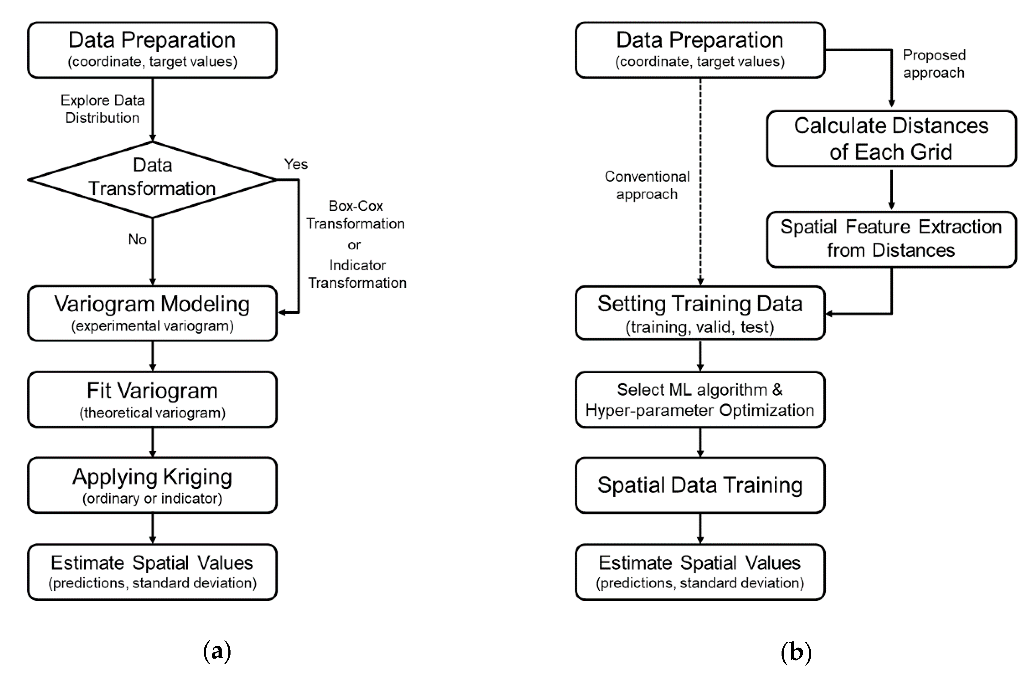
3. Methodology
3.1. Data Preparation & Processing
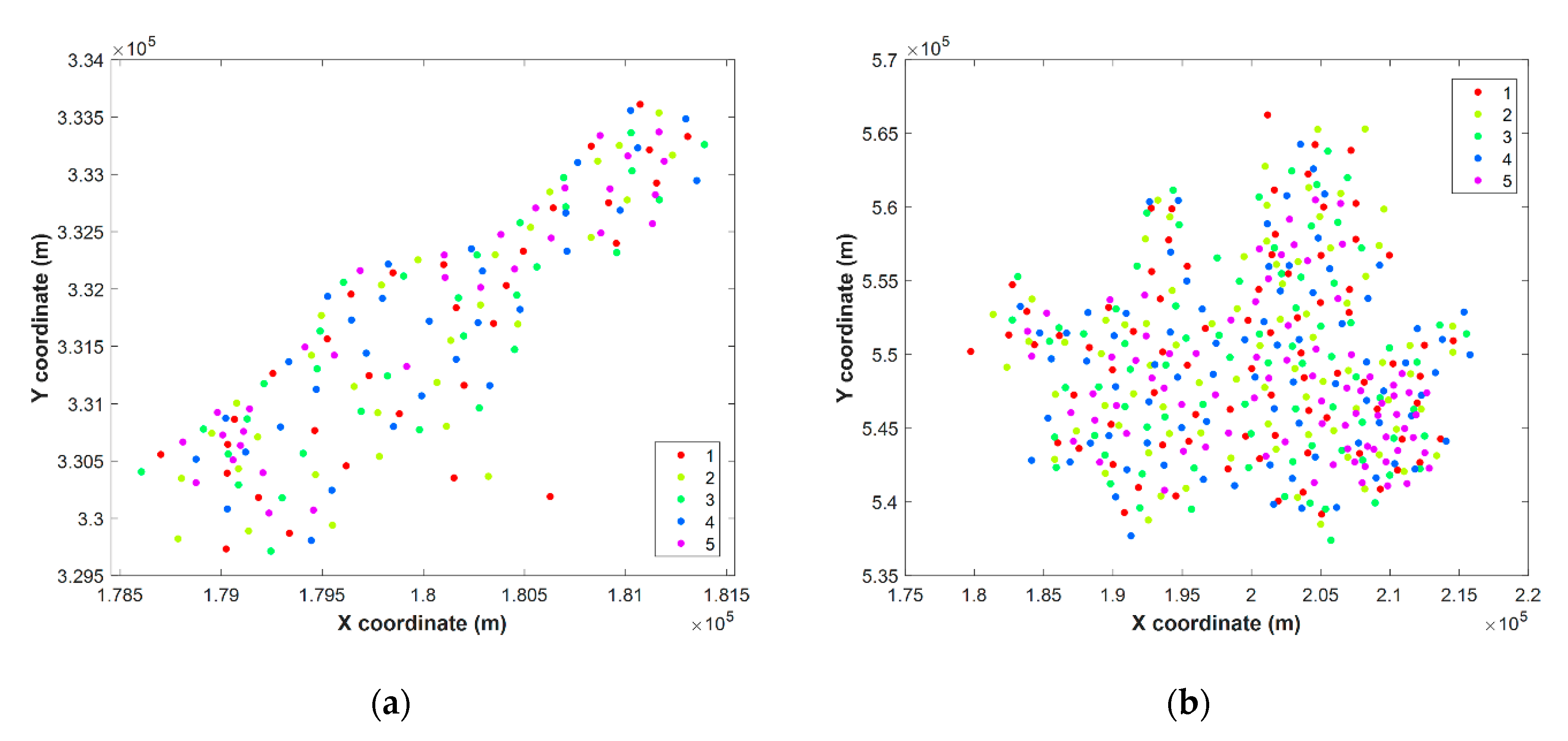
3.2. Data Partitioning
3.3. Machine Learning Algorithm and Hyper-Parameter Optimization
3.4. Training and Estimation of Spatial Data
4. Experiment
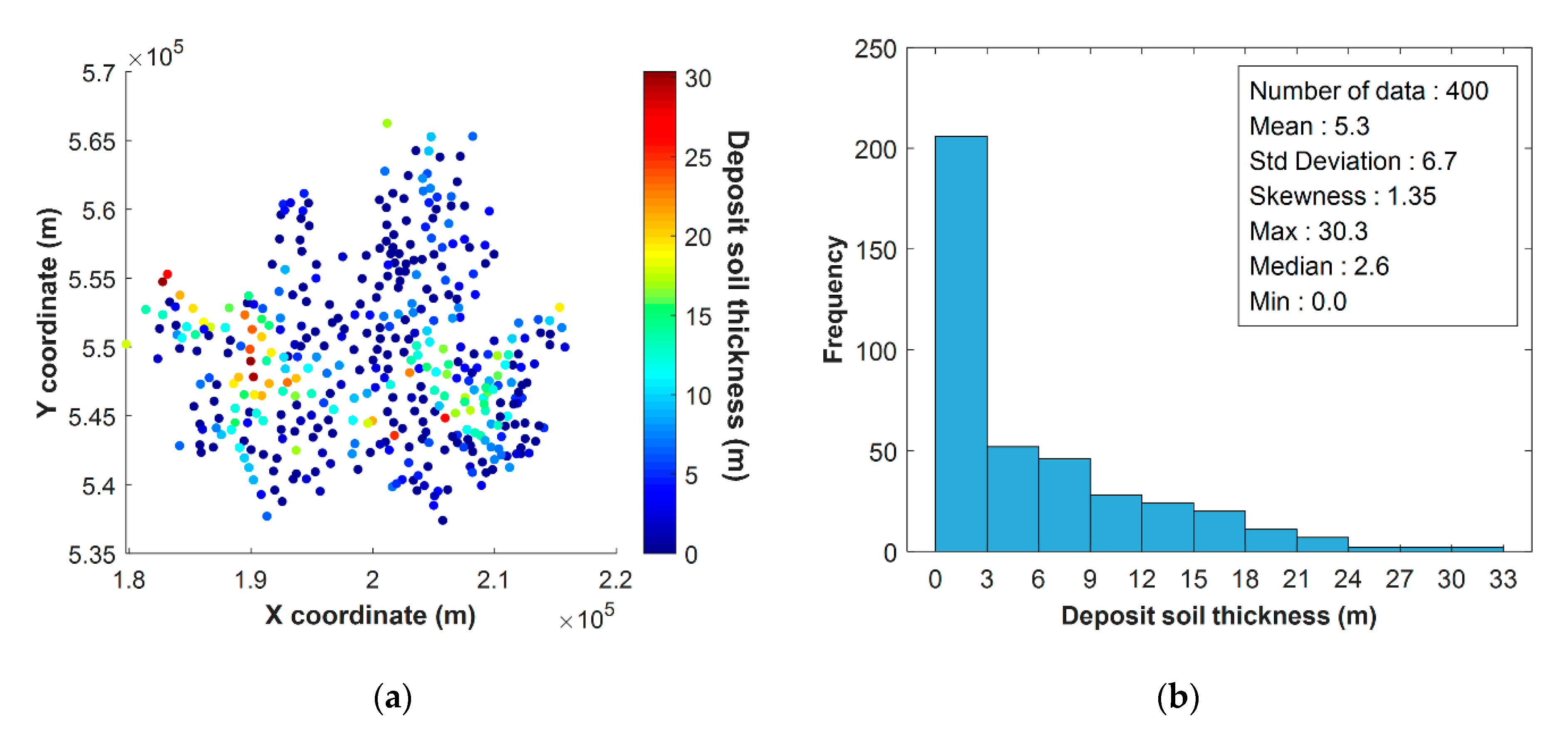
4.1. Dataset
4.2. Experimental Setup
4.3. Cross-Validation Method
4.4. Model Performance Criteria
5. Results and Discussion
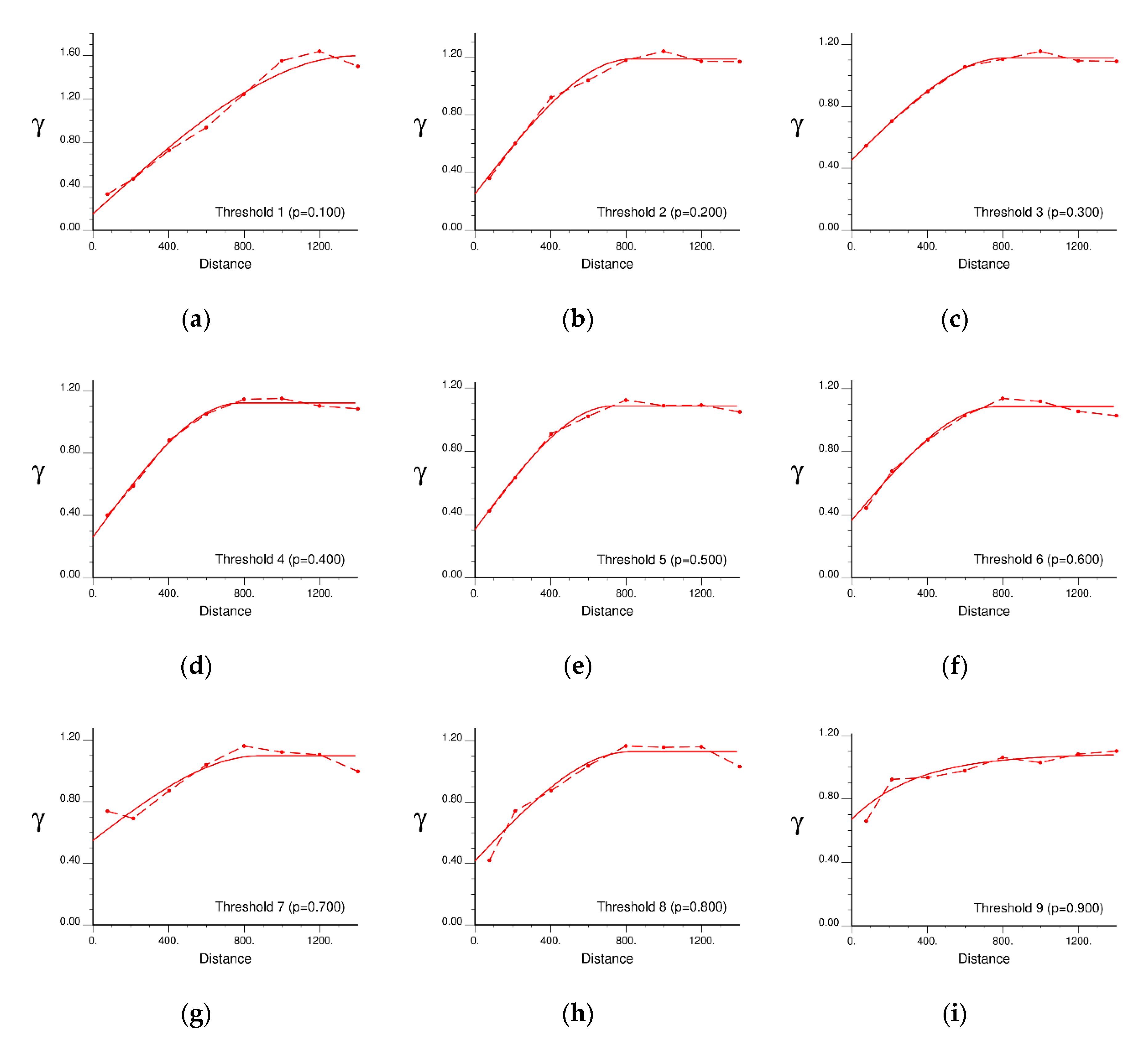
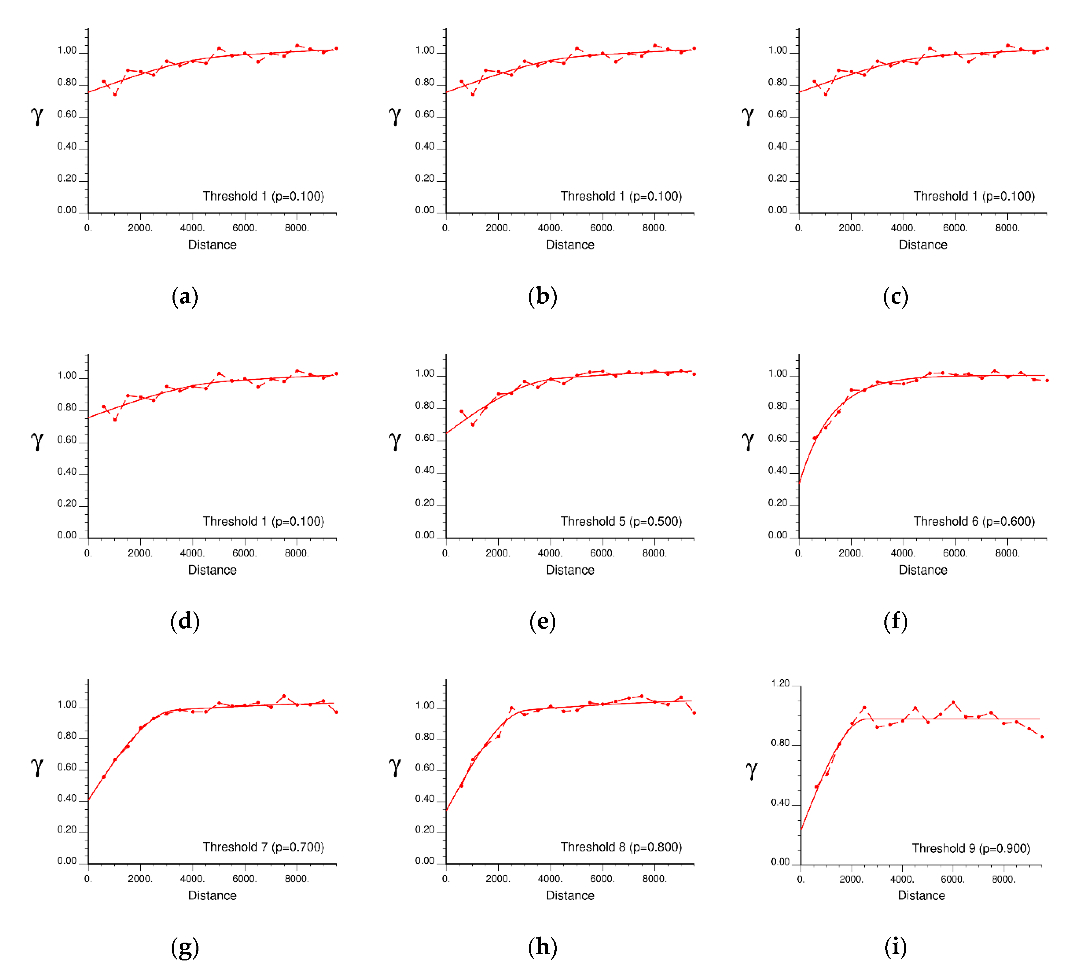
5.1. Variogram Modelling for IK
5.2. Optimization of the Number of PCs
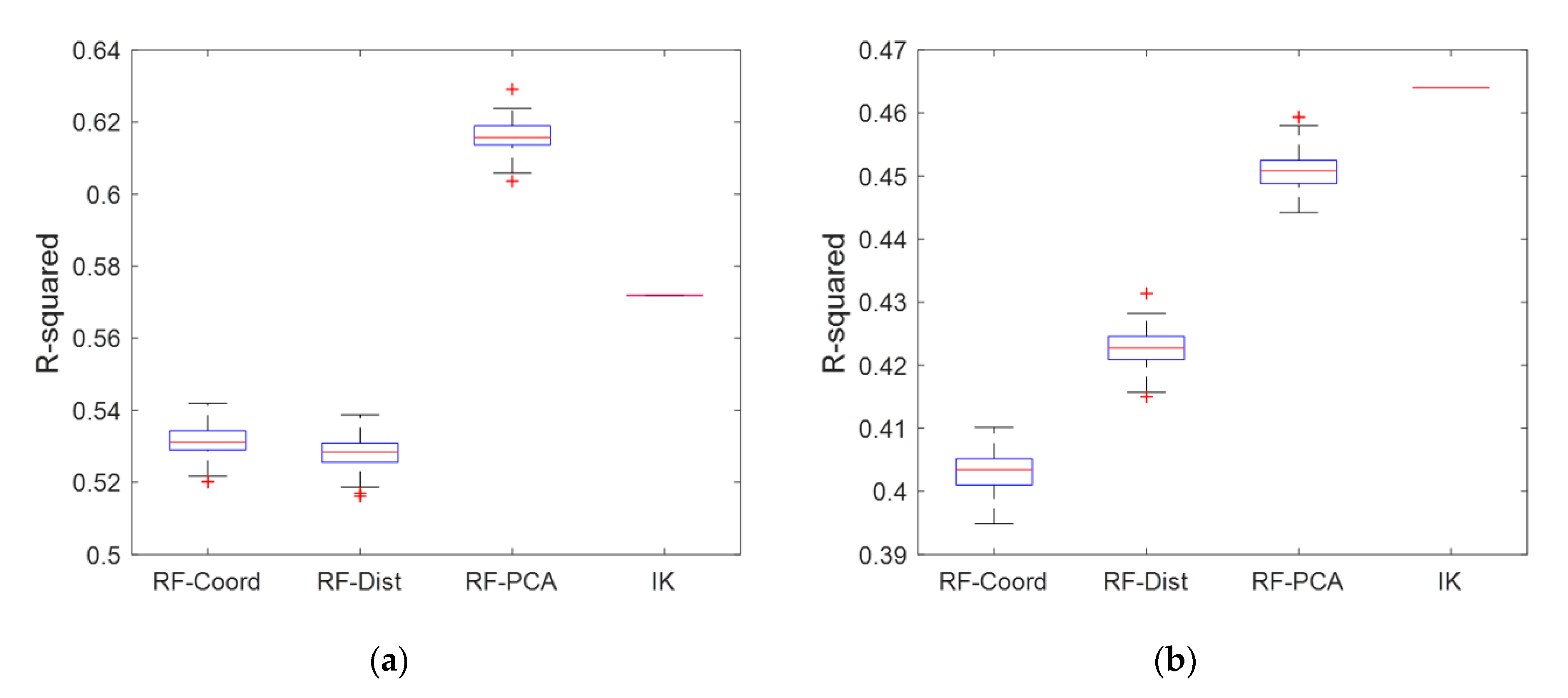
5.3. Validation of Prediction Performances
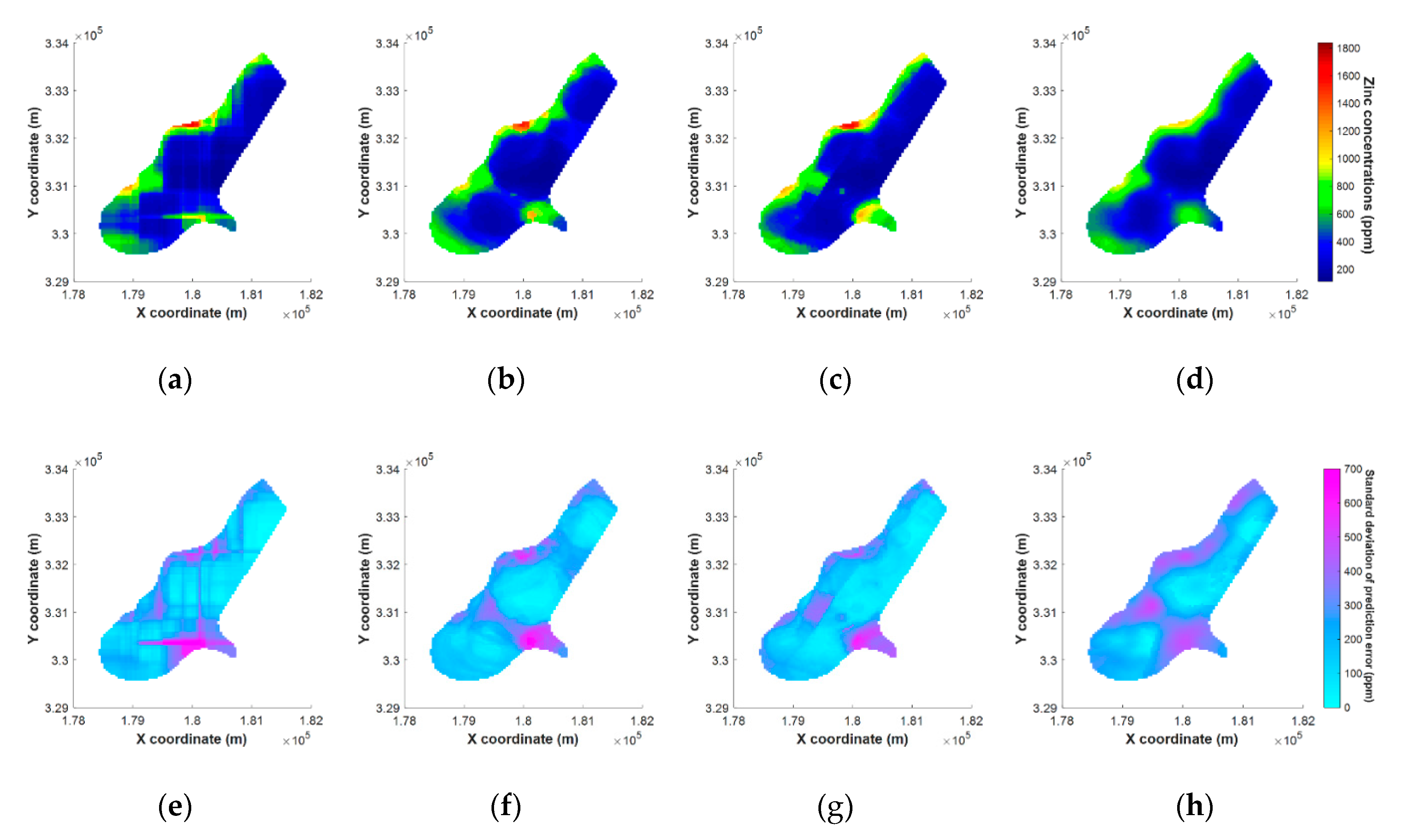
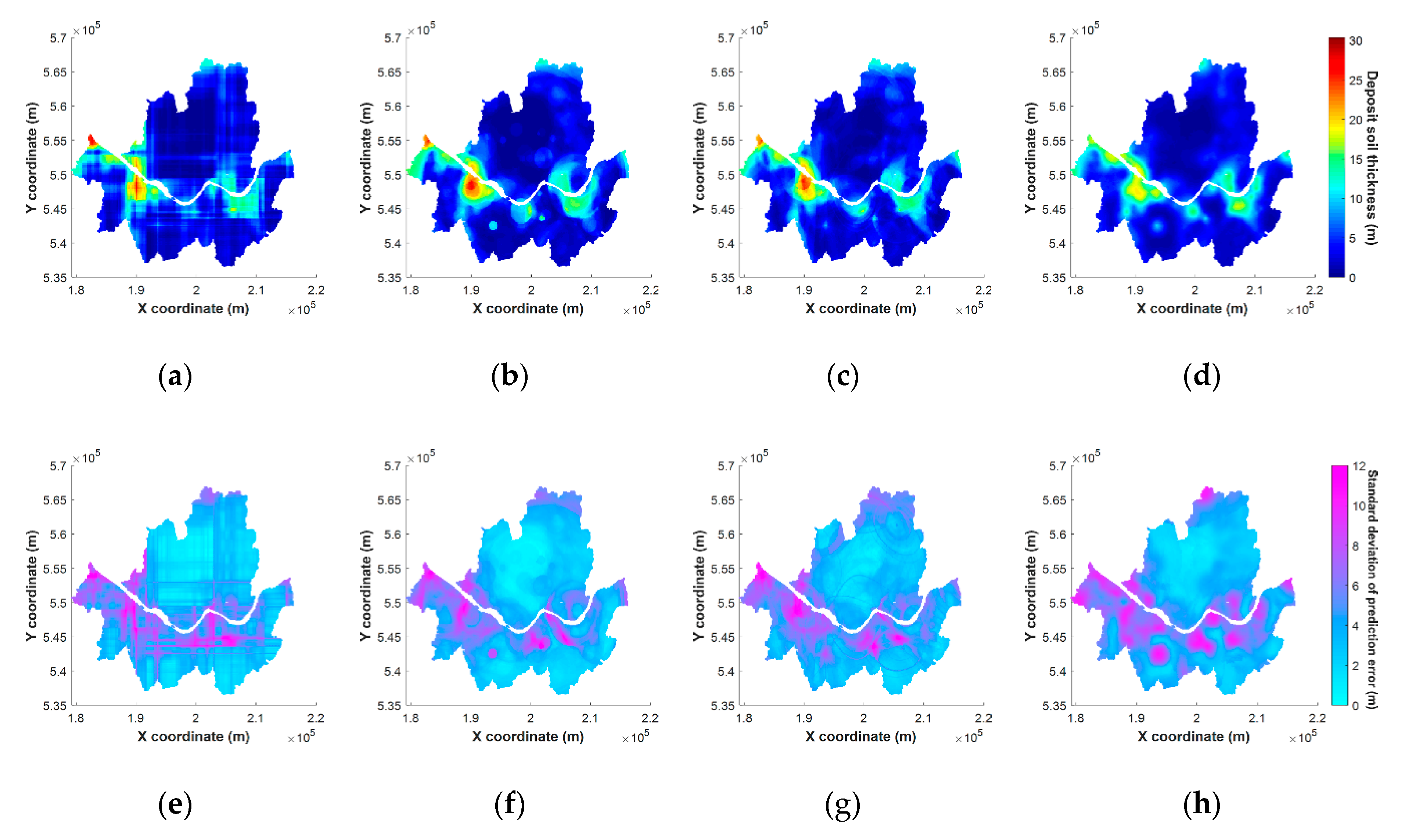
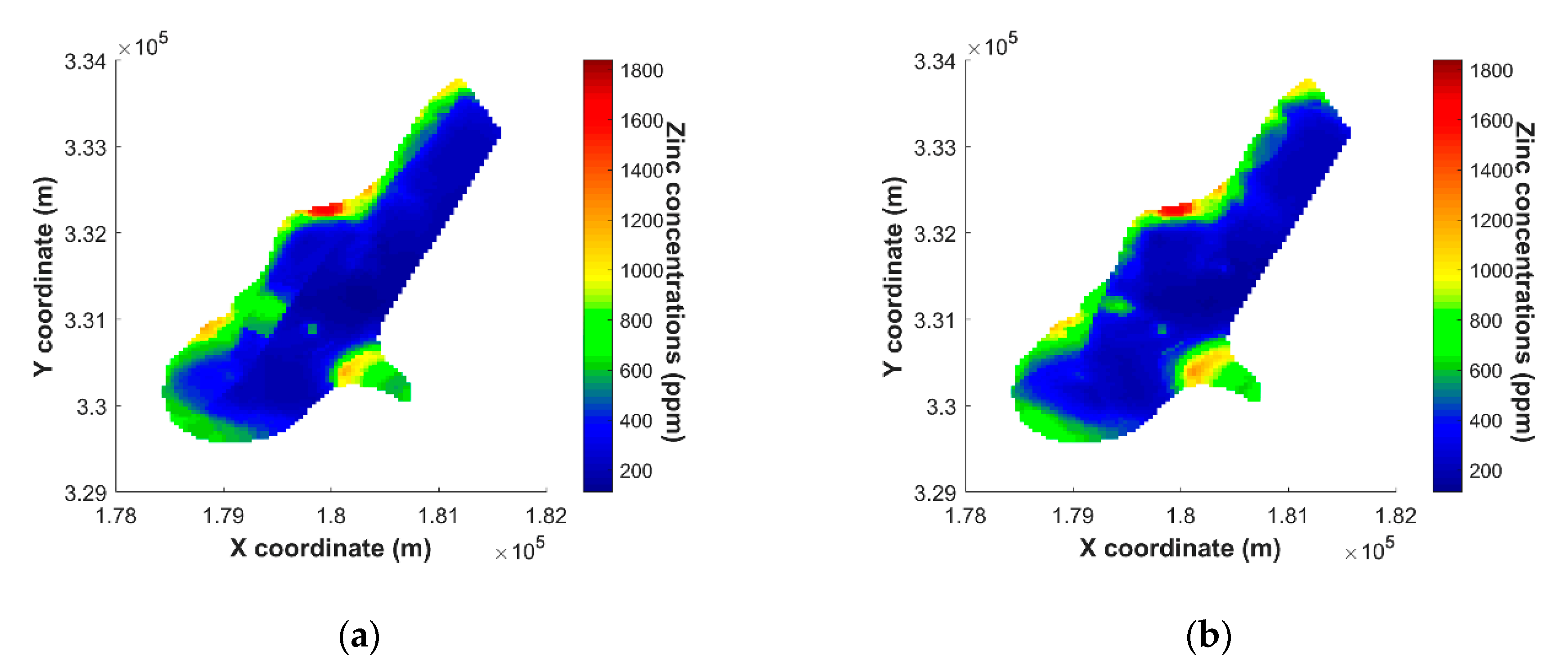
5.4. Results of Mapping on Spatial Grids
5.5. Effects Using Extracted PCs for Spatial Prediction
6. Conclusions
- Spatial estimation through MLA does not require assumptions about stationarity and variogram modelling. Moreover, additional transformation and back transformation for target variables are not required.
- Spatial correlation of data could be considered by using the distance vector as an input in the MLA. By applying PCA to the distance vector, it was possible to reduce the complexity of the input variable. Due to this, the computational cost of MLA is reduced, and the spatial estimation performance could increase.
- These results were obtained using only the coordinates for spatial estimation, without the addition of other covariates. Therefore, the proposed methodology can be used as a method for improving the performance of estimation in problems where there is no information available other than location information of sample data when using MLA.
- As a result of the application of the proposed methodology, the spatial estimation performance has improved, but artifacts have occurred according to the characteristics of the tree-based algorithm during the mapping process, which may vary depending on the spatial distribution of the target data. In future works, we should compare the results of applying the proposed method to MLA techniques other than RF, or study how to mitigate these effects in other ways.
- The computational cost of RF was reduced by applying PCA, but a direct comparison of computation cost was not conducted because a large dataset was not used. In future studies, we will apply the proposed method for a large point dataset and study the cost-effectiveness.
- The future studies can include the exploration of the application and effects of various techniques that can be used as a tool to extract spatial features other than PCA.
Author Contributions
Funding
Acknowledgments
Conflicts of Interest
References
- Krige, D.G. A statistical approach to some basic mine valuation problems on the Witwatersrand. J. S. Afr. I. Min. Metal. 1951, 52, 119–139. [Google Scholar] [CrossRef]
- Cressie, N. The origins of kriging. Math. Geosci. 1990, 22, 239–252. [Google Scholar] [CrossRef]
- Isaaks, E.H.; Srivastava, R.M. An Introduction to Applied Geostatistics; Oxford University Press: New York, NY, USA, 1989; ISBN 978-0-1950-5013-4. [Google Scholar]
- Goovaerts, P. Geostatistics for Natural Resources Evaluation; Oxford University Press: New York, NY, USA, 1997; ISBN 978-0-1951-1538-3. [Google Scholar]
- Deutsch, C.V.; Journel, A.G. GSLIB: Geostatistical Software Library and User’s Guide, 2nd ed.; Oxford University Press: New York, NY, USA, 1998; ISBN 978-0-1951-0015-0. [Google Scholar]
- Breiman, L. Random forests. Mach. Learn. 2001, 45, 5–32. [Google Scholar] [CrossRef] [Green Version]
- Liaw, A.; Wiener, M. Classification and regression by random forest. R News 2002, 2, 18–22. [Google Scholar]
- Wright, M.N.; Ziegler, A. Ranger: A fast implementation of random forests for high dimensional data in C++ and R. J. Stat. Softw. 2017, 77. [Google Scholar] [CrossRef] [Green Version]
- Hengl, T.; Heuvelink, G.B.M.; Kempen, B.; Leenaars, J.G.B.; Walsh, M.G.; Shepherd, K.D.; Sila, A.; MacMillan, R.A.; de Jesus, J.M.; Tamene, L.; et al. Mapping soil properties of Africa at 250 m resolution: Random forests significantly improve current predictions. PLoS ONE 2015, 10, e0125814. [Google Scholar] [CrossRef]
- Nussbaum, M.; Spiess, K.; Baltensweiler, A.; Grob, U.; Keller, A.; Greiner, L.; Schaepman, M.E.; Papritz, A. Evaluation of digital soil mapping approaches with large sets of environmental covariates. Soil 2018, 4, 1–22. [Google Scholar] [CrossRef] [Green Version]
- Georganos, S.; Grippa, T.; Gadiaga, A.N.; Linard, C.; Lennert, M.; Vanhuysse, S.; Mboga, N.; Wolff, E.; Kalogirou, S. Geographical random forests: A spatial extension of the random forest algorithm to address spatial heterogeneity in remote sensing and population modelling. Geocarto Int. 2019. [Google Scholar] [CrossRef] [Green Version]
- Hengl, T.; Nussbaum, M.; Wright, M.N.; Heuvelink, G.B.M.; Graler, B. Random forest as a generic framework for predictive modeling of spatial and spatio-temporal variables. PeerJ 2018, 6. [Google Scholar] [CrossRef] [Green Version]
- Juel, A.; Groom, G.B.; Svenning, J.C.; Ejrnaes, R. Spatial application of random forest models for fine-scale coastal vegetation classification using object based analysis of aerial orthophoto and DEM data. Int. J. Appl. Earth Obs. 2015, 42, 106–114. [Google Scholar] [CrossRef]
- Meyer, H.; Reudenbach, C.; Hengl, T.; Katurji, M.; Nauss, T. Improving performance of spatio-temporal machine learning models using forward feature selection and target-oriented validation. Environ. Model. Softw. 2018, 101, 1–9. [Google Scholar] [CrossRef]
- Meyer, H.; Reudenbach, C.; Wöllauer, S.; Nauss, T. Importance of spatial predictor variable selection in machine learning applications—Moving from data reproduction to spatial prediction. Ecol. Model. 2019, 411. [Google Scholar] [CrossRef] [Green Version]
- Valavi, R.; Elith, J.; Lahoz-Monfort, J.J.; Guillera-Arroita, G. BlockCV: An r package for generating spatially or environmentally separated folds for k-fold cross-validation of species distribution models. Methods Ecol. Evol. 2019, 10, 225–232. [Google Scholar] [CrossRef] [Green Version]
- Behrens, T.; Schmidt, K.; Rossel, R.A.V.; Gries, P.; Scholten, T.; MacMillan, R.A. Spatial modelling with Euclidean distance fields and machine learning. Eur. J. Soil Sci. 2018, 69, 757–770. [Google Scholar] [CrossRef]
- Journel, A.G. Nonparametric estimation of spatial distributions. Math. Geosci. 1983, 15, 445–468. [Google Scholar] [CrossRef]
- Goovaerts, P. AUTO-IK: A 2D indicator kriging program for the automated non-parametric modeling of local uncertainty in earth sciences. Comput. Geosci. 2009, 35, 1255–1270. [Google Scholar] [CrossRef] [PubMed] [Green Version]
- Remy, N.; Boucher, A.; Wu, J. Applied Geostatistics with SGeMS: A User’s Guide; Cambridge University Press: New York, NY, USA, 2009; ISBN 978-1-1074-0324-6. [Google Scholar]
- Ho, T.K. The random subspace method for constructing decision forests. IEEE TPAMI 1998, 20, 832–844. [Google Scholar]
- Hastie, T.; Tibshirani, R.; Friedman, J. The Elements of Statistical Learning: Data Mining, Inference, and Prediction, 2nd ed.; Springer: New York, NY, USA, 2013; ISBN 978-1-4614-6848-6. [Google Scholar]
- Pearson, K. LIII. On lines and planes of closest fit to systems of points in space. London, Edinburgh Dublin Philos. Mag. J. Sci. 1901, 2, 559–572. [Google Scholar] [CrossRef] [Green Version]
- Hotelling, H. Analysis of a complex of statistical variables into principal components. J. Educ. Psychol. 1933, 24, 417. [Google Scholar] [CrossRef]
- Jolliffe, I.T. Principal Component Analysis, 2nd ed.; Springer: New York, NY, USA, 2002; ISBN 978-0-387-95442-4. [Google Scholar]
- Wuttichaikitcharoen, P.; Babel, M. Principal component and multiple regression analyses for the estimation of suspended sediment yield in ungauged basins of Northern Thailand. Water 2014, 6, 2412–2435. [Google Scholar] [CrossRef] [Green Version]
- Iwamori, H.; Yoshida, K.; Nakamura, H.; Kuwatani, T.; Hamada, M.; Haraguchi, S.; Ueki, K. Classification of geochemical data based on multivariate statistical analyses: Complementary roles of cluster, principal component, and independent component analyses. Geochem. Geophys. 2017, 18, 994–1012. [Google Scholar] [CrossRef]
- Kang, B.; Jung, H.; Jeong, H.; Choe, J. Characterization of three-dimensional channel reservoirs using ensemble Kalman filter assisted by principal component analysis. Pet. Sci. 2019, 17, 182–195. [Google Scholar] [CrossRef] [Green Version]
- Bailey, S. Principal component analysis with noisy and/or missing data. Publ. Astron. Soc. Pac. 2012, 124, 1015. [Google Scholar] [CrossRef] [Green Version]
- Marinov, T.V.; Mianjy, P.; Arora, R. Streaming principal component analysis in noisy setting. In Proceedings of the 35th International Conference on Machine Learning, PMLR 2018, Stockholm, Sweden, 10–15 July 2018; Volume 80, pp. 3413–3422. [Google Scholar]
- Meinshausen, N. Quantile regression forests. J. Mach. Learn. Res. 2006, 7, 983–999. [Google Scholar]
- Probst, P.; Boulesteix, A.-L. To tune or not to tune the number of trees in random forest. J. Mach. Learn. Res. 2018, 18, 1–18. [Google Scholar]
- Rikken, M.G.J. Soil Pollution with Heavy Metals: In Inquiry into Spatial Variation, Cost of Mapping and the Risk Evaluation of Copper, Cadmium, Lead and Zinc in the Floodplains of the Meuse West of Stein; The Netherlands: Field Study Report; University of Utrecht: Utrecht, The Netherlands, 1993. [Google Scholar]
- Kuhn, M.; Johnson, K. Applied Predictive Modeling, 1st ed.; Springer: New York, NY, USA, 2013; ISBN 978-1-4614-6848-6. [Google Scholar]


| Algorithms | Input Type | Applying PCA | Abbreviation |
|---|---|---|---|
| Indicator Kriging | Coordinate | No | IK |
| Random Forest | Coordinate | No | RF-Coord |
| Random Forest | Distance | No | RF-Dist |
| Random Forest | Distance | Yes | RF-PCA |
| Dataset | Threshold Value | Semi-Variogram Model | Nugget (m²) | Sill (m²) | Range (m) |
|---|---|---|---|---|---|
| Meuse | 1 (152 ppm) | Spherical | 0.1485 | 1.4499 | 1392.74 |
| 2 (187 ppm) | Spherical | 0.2503 | 0.9350 | 832.44 | |
| 3 (207 ppm) | Spherical | 0.4520 | 0.6623 | 817.70 | |
| 4 (246 ppm) | Spherical | 0.2586 | 0.8617 | 778.85 | |
| 5 (326 ppm) | Spherical | 0.3038 | 0.7826 | 728.13 | |
| 6 (442 ppm) | Spherical | 0.3624 | 0.7249 | 765.54 | |
| 7 (593 ppm) | Spherical | 0.5480 | 0.5493 | 882.68 | |
| 8 (741 ppm) | Spherical | 0.4164 | 0.7119 | 826.08 | |
| 9 (1022 ppm) | Exponential | 0.6712 | 0.4146 | 1044.20 | |
| Seoul | 1~4 (0 m) | Spherical (1st) | 0.7566 | 0.1560 | 5282.20 |
| Spherical (2nd) | 0.1172 | 12172.94 | |||
| 5 (2.6 m) | Spherical (1st) | 0.6459 | 0.2365 | 4214.28 | |
| Exponential (2nd) | 0.1692 | 13754.17 | |||
| 6 (4.8 m) | Exponential (1st) | 0.3343 | 0.2603 | 3685.97 | |
| Exponential (2nd) | 0.4127 | 3706.61 | |||
| 7 (7.3 m) | Spherical (1st) | 0.4080 | 0.5280 | 3343.64 | |
| Exponential (2nd) | 0.1201 | 19061.42 | |||
| 8 (11.1 m) | Spherical (1st) | 0.3410 | 0.5919 | 3107.19 | |
| Exponential (2nd) | 0.1549 | 19990.08 | |||
| 9 (15.6 m) | Spherical | 0.2364 | 0.7443 | 2580.06 |
| Dataset | Parameters | RF-Coord | RF-Dist | RF-PCA | IK | True |
|---|---|---|---|---|---|---|
| Meuse | Mean | 457.9 | 457.5 | 452.8 | 459.7 | 469.7 |
| Max | 1510.0 | 1416.5 | 1425.3 | 958.4 | 1839.0 | |
| Median | 427.2 | 396.2 | 383.7 | 435.7 | 326.0 | |
| Min | 145.1 | 132.0 | 144.7 | 133.0 | 113.0 | |
| Std. | 250.1 | 256.2 | 251.2 | 227.8 | 367.1 | |
| RMSE | 251.4 | 251.8 | 230.4 | 247.8 | - | |
| R-squared | 0.53 | 0.53 | 0.62 | 0.57 | - | |
| Seoul | Mean | 5.31 | 5.03 | 5.25 | 5.21 | 5.34 |
| Max | 21.02 | 21.26 | 21.20 | 19.35 | 30.34 | |
| Median | 4.10 | 3.68 | 3.82 | 4.03 | 2.60 | |
| Min | 0.00 | 0.02 | 0.13 | 0.00 | 0.00 | |
| Std. | 4.38 | 4.46 | 4.28 | 3.92 | 6.89 | |
| RMSE | 5.16 | 5.09 | 4.96 | 4.93 | - | |
| R-squared | 0.40 | 0.42 | 0.45 | 0.46 | - |
| Dataset | Parameters | RF-PCA 15 | RF-PCA 30 | RF-PCA 50 | RF-PCA 100 | True |
|---|---|---|---|---|---|---|
| Meuse | Mean | 452.8 | 445.5 | 438.2 | 426.3 | 469.7 |
| Max | 1425.3 | 1227.2 | 1123.9 | 1010.7 | 1839.0 | |
| Median | 383.7 | 386.8 | 388.8 | 373.6 | 326.0 | |
| Min | 144.7 | 147.7 | 158.9 | 168.8 | 113.0 | |
| Std. | 251.2 | 235.6 | 223.7 | 208.2 | 367.1 | |
| RMSE | 230.4 | 243.5 | 246.7 | 257.4 | - | |
| R-squared | 0.62 | 0.58 | 0.57 | 0.55 | - | |
| Seoul | Mean | 5.25 | 5.02 | 4.81 | 4.22 | 5.34 |
| Max | 21.20 | 19.87 | 19.78 | 18.28 | 30.34 | |
| Median | 3.82 | 3.74 | 3.72 | 3.20 | 2.60 | |
| Min | 0.13 | 0.07 | 0.21 | 0.34 | 0.00 | |
| Std. | 4.28 | 4.04 | 3.84 | 3.36 | 6.89 | |
| RMSE | 4.96 | 5.01 | 5.06 | 5.26 | - | |
| R-squared | 0.45 | 0.44 | 0.44 | 0.43 | - |
© 2020 by the authors. Licensee MDPI, Basel, Switzerland. This article is an open access article distributed under the terms and conditions of the Creative Commons Attribution (CC BY) license (http://creativecommons.org/licenses/by/4.0/).
Share and Cite
Ahn, S.; Ryu, D.-W.; Lee, S. A Machine Learning-Based Approach for Spatial Estimation Using the Spatial Features of Coordinate Information. ISPRS Int. J. Geo-Inf. 2020, 9, 587. https://0-doi-org.brum.beds.ac.uk/10.3390/ijgi9100587
Ahn S, Ryu D-W, Lee S. A Machine Learning-Based Approach for Spatial Estimation Using the Spatial Features of Coordinate Information. ISPRS International Journal of Geo-Information. 2020; 9(10):587. https://0-doi-org.brum.beds.ac.uk/10.3390/ijgi9100587
Chicago/Turabian StyleAhn, Seongin, Dong-Woo Ryu, and Sangho Lee. 2020. "A Machine Learning-Based Approach for Spatial Estimation Using the Spatial Features of Coordinate Information" ISPRS International Journal of Geo-Information 9, no. 10: 587. https://0-doi-org.brum.beds.ac.uk/10.3390/ijgi9100587